


1. Introduction
Atmospheric observations over 6 decades have revealed the occurrence and variability of Kelvin–Helmholtz instability (KHI) scales, character and consequences from the surface to over 100 km; see Fritts et al. (Reference Fritts, Wang, Lund and Thorpe2022). Similar observations over the same interval suggested significant roles for KHI throughout the oceans; e.g. Thorpe (Reference Thorpe2005). Only recently, however, have atmospheric observations at high altitudes yielded sufficiently high resolution to reveal larger-scale primary KH billows, smaller-scale secondary convective instabilities (CI) and/or KHI of individual KH billows and additional features arising from interactions among misaligned billow cores first identified in laboratory experiments and named ‘tubes and knots’ (Thorpe Reference Thorpe1973a,Reference Thorpeb). New imaging observations by Hecht et al. (Reference Hecht, Fritts, Gelinas, Rudy, Walterscheid and Liu2021), and surveys of earlier lower-resolution imaging, suggest that such multi-scale KHI dynamics are widespread and may have significant implications for energy dissipation and mixing throughout the atmosphere and oceans. Related ground-based polar mesospheric cloud (PMC) imaging by Baumgarten & Fritts (Reference Baumgarten and Fritts2014) and Fritts et al. (Reference Fritts, Baumgarten, Wan, Werne and Lund2014a) revealed additional evidence of secondary CI and KHI of KH billows. These studies also exhibit perturbations to billow cores driven by billow interactions suggestive of large-scale (Kelvin Reference Kelvin1880) waves, or ‘twist waves’ (Arendt, Fritts & Andreassen Reference Arendt, Fritts and Andreassen1997), that break up the axial coherence of KH billows and initiate their fragmentation.
Evidence for all of the responses noted above are seen in the direct numerical simulation (DNS) described by Fritts et al. (Reference Fritts, Wang, Lund and Thorpe2022). That study described both KH billow secondary CI and KHI, and two examples of tube and knot dynamics, such as revealed in the laboratory observations by Thorpe (Reference Thorpe1987, Reference Thorpe2002), Caulfield, Yoshida & Peltier (Reference Caulfield, Yoshida and Peltier1996) and Holt (Reference Holt1998), and the atmospheric observations cited above. The more significant dynamics in this DNS driving KH billow breakdown via tube and knot dynamics, and their cascade to smaller energy dissipation scales, include the following (also see figures 3 and 4 below):
(i) emerging vortex tubes ‘linking’ to adjacent KH billow cores where the billows are initially misaligned or discontinuous along their axes;
(ii) interactions among vortex tubes and KH billow cores where they ‘link’, forming knots that entwine them and drive strong and rapid subsequent vortex interactions;
(iii) axial and radial vortex tube and billow core amplitude and phase distortions driven by roughly orthogonal vortices resulting in vortex twist waves that propagate away from the knots along the tube(s) and billow core(s); and
(iv) successive additional, roughly orthogonal, vortex interactions that contribute to their fragmentation and cascade to smaller-scale vortices thereafter.
Also seen in close proximity to these sites are enhanced secondary KHI and vortex tubes in the intensified vortex sheets due to their deformation and stretching around the tube and knot events, and enhanced secondary CI in the intensified KH billow interiors. However, these latter dynamics arise at very much smaller scales, so cannot contribute to the large energy dissipation rates of primary interest here.
KH billow pairing occurs at early stages of the evolution over a limited spanwise extent, and following KH billow breakdown to turbulence at locations weakly impacted by the initial tube and knot dynamics; see figures 8 and 9 of Fritts et al. (Reference Fritts, Wang, Lund and Thorpe2022). Thus, in this DNS at least, billow pairing does not play a major role in enhanced energy dissipation.
Of the dynamics discussed above, those that appear to contribute most to rapid and intense turbulence transitions, strong energy dissipation and potential mixing in multi-scale KHI in the laboratory, the atmosphere and likely also in oceans and lakes, are vortex tubes, knots and twist waves arising on or between emerging misaligned and/or distorted billow cores in the multi-scale DNS performed by Fritts et al. (Reference Fritts, Wang, Lund and Thorpe2022). Of these, KHI tubes and knots were recognized to be important in early laboratory studies cited above. They also arose, but were poorly resolved and neither described nor quantified, in previous large-eddy simulations of unstratified shear flows having sufficiently large domains (Comte, Silvestrini & Begou Reference Comte, Silvestrini and Begou1998; Balaras, Piomelli & Wallace Reference Balaras, Piomelli and Wallace2001). Despite their apparent importance and frequent occurrence in geophysical flows, none of these dynamics are included in the ‘zoo’ of KHI secondary instabilities arising for KHI that exhibit no spanwise variability in phase or wavelength (Mashayek & Peltier Reference Mashayek and Peltier2012).
The KHI DNS described by Fritts et al. (Reference Fritts, Wang, Lund and Thorpe2022) is the first to examine KHI vorticity dynamics extending well into the viscous (dissipation) range, and resolving turbulence features at scales  ${\sim}3\text{--}10$ times the Kolmogorov scale, $\eta$, for a Reynolds number, $Re=5000$, that is sufficiently large to enable the various KHI secondary instabilities identified by Mashayek & Peltier (Reference Mashayek and Peltier2012, Reference Mashayek and Peltier2013) and the tube and knot dynamics enabled in a larger domain. Our purposes here are to employ these DNS results to identify and quantify the KHI dynamics that account for the major kinetic energy dissipation as a function of the initial tube and knot dynamics, and that occurs in their absence.
Our paper is organized as follows. The DNS model set-up, initial conditions and analysis methods are described in § 2. An overview of the KHI tube and knot dynamics described by Fritts et al. (Reference Fritts, Wang, Lund and Thorpe2022) is provided in § 3, including descriptions of the vorticity dynamics driving energy to smaller scales for the two primary tube and knot events employing three-dimensional (3-D) imaging. Section 4 describes (i) the energy dissipation rate,  $\epsilon$, evolution using horizontal and vertical cross-sections at the shear layer and spanwise locations highlighting the varying responses, (ii) relations between vorticity and $\epsilon$ for the two primary KHI tube and knot events, and (iii) exploration of the $\epsilon$ evolutions for these two cases and at a location largely without tube and knot influences using 3-D imaging from two perspectives. Probability density functions (PDFs), temporal evolutions and spectra of $\epsilon$ in various subdomains containing, and without, tube and knot dynamics are examined in § 5. A discussion of our results relative to previous related studies and our summary and conclusions are presented §§ 6 and 7.
2. Fourier spectral model and simulation parameters
Fritts et al. (Reference Fritts, Wang, Lund and Thorpe2022) employed a high-radix spectral model to solve the Boussinesq Navier–Stokes equations in a domain enabling the emergence of misaligned KH billows leading to tube and knot dynamics. The domain had dimensions  $(X,Y,Z)/L=(3,9,3)$, with $x$,
$x$,  $y$ and $z$ along the mean shear (streamwise), spanwise and vertical, respectively, in order to enable KH billow misalignments arising from random initial noise (see below). The domain and initial shear depth were chosen to enable 3 or 4 initial KH billows (with a nominal wavelength $\lambda _h \sim L$) to emerge at finite amplitudes along $x$. The domain extent in $y$ allowed significant initial KHI phase variations along $y$ for 10 initial noise seeds, one of which having weaker phase variations was selected for our DNS.
The initial mean wind and stratification were specified as
 \begin{equation} U(z) = U_0\cos\left(\frac{{\rm \pi} z}{Z}\right)\tanh\left(\frac{z}{h}\right) \end{equation}
and
 \begin{equation} N^2(z) = N_0^2 + (N_m^2 - N_0^2) {\rm sech}^2\left(\frac{z}{h}\right) \end{equation}
to approximate an environment due to a steepened inertia–gravity wave, such as often arise in the atmosphere and oceans, as shown in figure 1. Here,  $U_0$ is the half-shear velocity difference, $z=0$ at the domain centre, $Z$ is the domain depth, $h=0.07$ L, $N_0^2=10^{-4}\,{\rm s}^{-2}$, $N_m^2=8N_0^2$ with $N^2=(g/T)({\rm d} T/{\rm d} z)$ for temperature $T$, a buoyancy period $T_b=2{\rm \pi} /N_m=222$ s and potential temperature $\theta =T$ for a Boussinesq fluid. Remaining parameters are defined by a minimum Richardson number, $Ri=N_m^2/({\rm d} U/{\rm d} z)^2=0.1$, Reynolds number, $Re=U_0h/\nu =5000$, kinematic viscosity $\nu$ and Prandtl number, $Pr=1$, so as to require the same resolution for velocity and temperature fields, given the major computational resources needed to perform the DNS.

Figure 1. Initial fields in  $U(z)$, $\theta (z)$, $N^2(z)$ and $Ri$ employed for the multi-scale KHI DNS intended to approximate a large-amplitude gravity wave structure.
The DNS was ensured by requiring a minimum spatial resolution  ${\rm \Delta} {x}<1.8\eta$ defined by a maximum mean $\overline \epsilon$ assessed over every $x$,
$x$,  $y$ and $z$ plane for a minimum Kolmogorov scale,
 \begin{equation} \eta=(\nu^3/\epsilon)^{1/4}, \end{equation}
where
 \begin{equation} \epsilon=2\nu\langle S_{ij}S_{ij}\rangle\end{equation}
and
 \begin{equation} S_{ij}=(\partial u_i/\partial x_j+\partial u_j/\partial x_i)/2. \end{equation}
 The DNS was performed for a minimum Richardson number,  $Ri=0.1$, and a Reynolds number, $Re=5000$, to allow secondary CI and KHI of individual KH billows to arise and compete with the tube and knot dynamics initiated by interacting KH billows. As noted by Fritts et al. (Reference Fritts, Wang, Lund and Thorpe2022), responses include multiple features closely resembling those revealed in the laboratory and more recent atmospheric observations cited above. The DNS employed a non-divergent white noise in the velocity field with $u_{rms}=U_0\times 10^{-5}$ to enable KH billows having variable wavelengths, $\lambda _h(x,y)$, and phases, $\phi (x,y)$, with billow cores roughly normal to the mean shear. A second noise seed was also introduced prior to the initial transition to turbulence to approximate the influences of pre-existing turbulence and ensure emergence of significant secondary KH billow CI and KHI to compete with the emerging tube and knot dynamics.
In order to relate our exploration of the energetics and energy dissipation accompanying these KHI dynamics to the vorticity dynamics discussed by Fritts et al. (Reference Fritts, Wang, Lund and Thorpe2022), we also employ the quantity  $\lambda _2$ shown by Jeong & Hussain (Reference Jeong and Hussain1995) to accurately reveal vorticity having strong rotational character. As described by these authors, $\lambda _2$ is the intermediate eigenvalue of the tensor $\boldsymbol {H} = \boldsymbol {S}^2 + \boldsymbol {R}^2$, where $\boldsymbol {S}$ and $\boldsymbol {R}$ are the strain and rotation rate tensors, respectively, and negative $\lambda _2$ imply rotational motions. Comparisons of $\lambda _2$ and $\epsilon$ are employed below to reveal the vorticity dynamics driving emerging $\epsilon$ at small scales.
3. Overview of the multi-scale KHI tube and knot dynamics
The multi-scale KHI dynamics described by Fritts et al. (Reference Fritts, Wang, Lund and Thorpe2022) are summarized for reference with two-dimensional (2-D) cross-sections of  $T^\prime /T_0(x,y)$ at $z=0$ and of $T/T_0(x,z)$ at $y/L=2$, 3, 4, 5.5 and 8.5 and at 2.5, 3.5, 4.5 and 5.5 $T_b$ in the upper and lower panels of figure 2. Times are with respect to an initial time, defined as 0 $T_b$, having a maximum $T^\prime /T_0<0.0015$ and exhibiting weak optimal perturbations prior to their projections onto initial, coherent KHI phases aligned roughly along $y$. They extend to the later stages of initial billow breakdown and initial restratification. The two sets of cross-sections reveal the following features of the dynamics relevant to our analyses here:
(i) overturning KH billows arise by 2.5 $T_b$ exhibiting regions of significant phase kinks or misalignments yielding ${\rm d}\phi /{{\rm d}y}>0$ along their axes due to the initial noise seed;
(ii) initial links by emerging vortex tubes penetrating the
$z=0$ plane to adjacent KH billows that are discontinuous or misaligned, which intensify strongly by 3.5$T_b$;(iii) responses to the tube and knot dynamics at 3.5
$T_b$ showing early stages of turbulence generation and enhanced initial secondary KHI along the stratified sheets between adjacent billows and secondary CI in the billow interiors, especially at $y/L\sim 1.5\text {--}6$;(iv) rapid expansion of turbulence in the regions of initial tubes and knot dynamics, and accompanying the secondary KHI and CI between and within the KH billows spanning the
$y$ domain prior to 4.5$T_b$; and(v) further billow breakdown, pairing and merging resulting in a turbulent mixing layer at the initial stages of restratification, especially at
$y/L=2$–5.5 (last panels at 5.5$T_b$).


Figure 2. The 2-D cross-sections of  $T^\prime /T_0(x,y)$ at $z=0$ (a) and $T/T_0(x,z)$ at $y/L=2$, 3, 4, 5.5 and 8.5 (b, bottom to top) at 2.5, 3.5, 4.5 and 5.5 $T_b$ (left to right). Colour scales for $T^\prime /T_0(x,y)$ are shown at upper right in each panel. Black and white rectangles in the upper panel at 3.5 $T_b$ show two local regions in which the dynamics will be examined in detail below.
Two examples of the tube and knot vorticity dynamics described by Fritts et al. (Reference Fritts, Wang, Lund and Thorpe2022) driving the strongest  $\epsilon$ evolutions are shown in figures 3 and 4. These occur in the DNS regions 1 and 2 shown in figure 2. Region 1 (black dashed rectangle) spans the $x$ domain boundary and contains a single vortex tube that attaches to the outer edges of two adjacent KH billows. Region 2 (white dashed rectangle) contains two vortex tubes displaced along $x$ linking to a single KH billow in close proximity. Not seen in this DNS are misaligned and discontinuous KH billows along their axes, as simulated by Fritts et al. (Reference Fritts, Wieland, Lund, Thorpe and Hecht2021) using a compressible code with an LES constraint at small scales.

Figure 3. The 3-D  $\lambda _2$ imaging in region 1 (black rectangle at bottom spanning the $x$ domain boundary in figure 2) showing the evolution of a vortex tube linking two adjacent KH billow cores viewed from above. Blue/green (yellow/red) colours denote smaller (larger) negative $\lambda _2$. Small-scale approximately linear features outside the tube and knot dynamics emerging at 3.5 $T_b$ are secondary KHI; weaker features at lower left seen best at 3.7 $T_b$ are secondary CI in the outer KH billows. Axes are shown at upper left. Sites labelled $a$–
$a$– $g$ are cited in the text.

Figure 3 shows the initial evolution of a single vortex tube in region 1 linking two adjacent KH billows where they have significant initial  ${\rm d}\phi /{{\rm d}y}>0$. The vortex tube has components $\zeta _i=(\boldsymbol {\nabla }\times V)_i$ and magnitude $\zeta =(\zeta _i^2)^{1/2}$, evolves on the vortex sheet between adjacent KH billows and is oriented from lower right to upper left. The two KH billow cores have roughly orthogonal orientations with vorticity oriented from lower left to upper right; they only have significant $\lambda _2$ at $\sim$3 $T_b$ where stretched by the vortex tube (labelled $a$). The vortex tube ‘links’ to the billow cores (labelled $b$) at their outer edges, wrapping below (above) the billow core at upper left (lower right) to form initial vortex knots (labelled $c$). The knots exhibit rapid and strong interactions including mutual vortex tube and billow core entwining (with spanwise vorticity, $\zeta _y>0$). These dynamics excite vortex twist waves seen emerging by 3.3 $T_b$ (labelled $d$) that propagate away from the knots along the vortex tube (and billow cores), account for the vortex tube weakening and breakdown (labelled $e$) and drive a rapid cascade to smaller-scale twist waves and turbulence thereafter. Additional small-scale vortices (labelled $f$) seen emerging along the weak, invisible billow cores and the intermediate vortex sheet at 3.5 $T_b$ (with $\zeta _x<0$), are much weaker secondary KHI. Roughly orthogonal, small-scale vortex tubes emerging by 3.7 $T_b$ (with $\zeta _x>0$) are secondary vortex tubes that together with the secondary KHI drive secondary tube and knot dynamics at $\sim$10–20 times smaller scales (labelled $g$).
$g$).
Figure 4 shows the initial evolution of two vortex tubes (labelled  $a$) in region 2 linking to a single KH billow core (labelled $b$) where it has a significant initial phase variation along $y$. In this case, the tubes drive more rapid dynamics over the same interval shown in figure 3 because both vortex tubes have $\zeta _y>0$ and $\zeta _x<0$, but overlie and underlie the billow core at smaller and larger $y$, respectively. Hence, they result in much stronger vortex tube and billow core knots (labelled $c$) driving interactions that induce strong differential stretching and compression along the KH billow core, and rapid large-scale twist-wave generation (labelled $d$). Subsequent twist-wave propagation along the tubes and KH billow core contribute to their weakening and fragmentation thereafter (labelled $e$). As in region 1, these tube and knot dynamics also drive smaller-scale secondary KHI, vortices and tube and knot dynamics on the intensifying vortex sheets (labelled $f$ and $g$).
$g$).
Mutual interactions also impact the vortex tubes and excite additional twist waves that propagate along, twist and unravel the vortex tubes (see sites labelled  $d$ and $e$ in both figures). Twist-wave generation is much more aggressive in region 2, as seen by comparing the figures at 3.3 $T_b$ and thereafter. As in region 1, these tube and knot interactions enable secondary KHI in the distorted vortex sheets surrounding this event. Significantly, both events yield initial turbulence by 3.5 $T_b$ and strong turbulence within $\sim$0.7 $T_b$ of the onset of strong tube and knot interactions, and prior to the emergence of significant secondary CI and KHI accompanying KH billow evolutions without strong tube and knot dynamics.
4. Energy dissipation rates in multi-scale KHI dynamics
We examine here the  $\epsilon$ field evolution driven by the vorticity dynamics revealed in the 2-D and 3-D $\lambda _2$ fields described by Fritts et al. (Reference Fritts, Wang, Lund and Thorpe2022). The $\epsilon (x,y)$ and $\epsilon (x,z)$ evolutions paralleling those for $\zeta$, $T'/T$ and $T/T_0$ in Fritts et al. (Reference Fritts, Wang, Lund and Thorpe2022) are described in § 4.1. Section 4.2 compares 3-D imaging of $\lambda _2$ and $\epsilon$ to reveal the consequences of the vorticity dynamics driving small-scale energy dissipation in regions 1 and 2. More extensive 3-D imaging of $\epsilon$ from two perspectives is employed to explore and inter-compare these evolutions in regions with and without tube and knot dynamics in § 4.3.
4.1. The $\epsilon$ evolution in horizontal and vertical planes

Shown in figures 5 and 6 are 2-D cross-sections of  $\epsilon$ corresponding to those for temperature in figure 2. These fields correspond closely to those for $|\zeta |$ in figures 7 and 8 of Fritts et al. (Reference Fritts, Wang, Lund and Thorpe2022), but note the absence of $\epsilon$ in the tube and billow cores, which have non-zero $|\zeta |$ but $\epsilon \sim 0$. The $\epsilon (y,z)$ cross-sections at $x/L=0$ and 1.5 and at 4, 5, 6, 7 and 10 $T_b$ are shown in figure 7 to reveal larger-scale responses to tube and knot dynamics emerging at later times. For reference, the $\epsilon$ magnitudes shown correspond to KH billows having $\lambda _h\sim$2 km at an altitude of $\sim$65 km in the atmosphere and $\lambda _h\sim$2 m in the oceans.

Figure 5. As in figure 2 showing 2-D cross-sections of  $\epsilon (x,y)$ and $\epsilon (x,z)$ intensities at $z=0$ and the $y/L$ shown with white lines from 3–4 $T_b$ at 0.5 $T_b$ intervals. A common logarithmic colour scale for all panels is shown at top left, and is saturated so as to reveal a broad range of intermediate $\epsilon$ magnitudes. Units are ${\rm m}^2\,{\rm s}^{-3}$ based on an assumed KH $\lambda _h=L=2$ km for representative observations in the stratosphere.


Figure 7. As in figure 5 for  $\epsilon (y,z)$ cross-sections at $x/L=0$ and 1.5 (a,b) and from 4–10 $T_b$ (top to bottom in each panel). The colour scale is as in figure 5. Note the undulations of the turbulent layer along $y$ increasing to $\sim$6 $T_b$ and decreasing as $\epsilon$ decreases thereafter.
The cross-sections in figures 5 and 6 at 3 $T_b$ reveal increasing $\epsilon$ in the strongly stratified vortex sheets between adjacent billows where they exhibit significant phase variations, ${\rm d}\phi /{{\rm d}y}$, along $y$. Larger local ${\rm d}\phi /{{\rm d}y}$ lead to initial vortex tubes due to roll-up of the intermediate vortex sheets due to their differential stretching by the rearward, at smaller $x$ (forward, at larger $x$) billows at larger (smaller) $y$ relative to the weaker, larger-scale ${\rm d}\phi /{{\rm d}y}>0$. Vortex tube cores have relatively uniform rotation, hence weak core $\epsilon$, at this stage. These evolving dynamics result in intensifying, larger-scale vortex tubes (relative to secondary KHI) on the vortex sheets, but having vorticity toward negative $x$ and positive $y$, as seen for the vortex tubes in figures 3 and 4. In all cases, regions of intensifying $\epsilon$ are consistent with vortex tubes linking adjacent or misaligned KH billow cores seen in the 3-D $\lambda _2$ imaging in Fritts et al. (Reference Fritts, Wang, Lund and Thorpe2022) at this time (also see § 5 below).
By 3.5 $T_b$, the vortex tubes seen at $(x,y)/L\sim (0.3,5.5)$, (1.1,5.4) and (2.8,3.6) evolving on the vortex sheets, and the adjacent KH billows, exhibit initial, localized turbulence. The two vortex tubes having larger cross-sections still have laminar cores, but that at $(x,y)/L\sim (1.1,5.4)$ is already fully turbulent at this time. Also seen are close associations of the vortex tubes with initial turbulent regions in adjacent billow cores. In all cases (due to ${\rm d}\phi /{{\rm d}y}>0$ at $y/L\sim 1.5$–8), vortex tubes exhibit clockwise rotation in the $(x,y)$ plane viewing from positive $z$. Consistent with the vortex dynamics seen in the laboratory (Thorpe Reference Thorpe1987, Reference Thorpe2002), the vortex tubes link to the far sides of adjacent billows in all cases. As a result, both figures exhibit localized and enhanced $\epsilon$ at the far sides of the KH billows to the upper left and/or lower right of the major vortex tubes seen to arise on the stratified braids at $z=0$ for the same reasons.
Also seen at 3.5 $T_b$ are emerging local $\epsilon$ maxima due to initial secondary KHI along the stratified braids between the larger KH billows where ${\rm d}\phi /{{\rm d}y}$ is large and they are in close proximity to the sites of tube and knot dynamics, see especially at $y/L\sim 2$–6 at the top of figure 5 and at $y/L=4$ and 5.5 at the bottom. Additional, small-scale 3-D structures exhibiting increasing $\epsilon$ are seen emerging in the outer billow cores where they are in close proximity to the initial tube and knot dynamics. At all of these sites, however, the small-scale secondary KHI and CI are laminar at this time due to their very small $Re$.
$Re$.
Figures 5 and 6 reveal that all the KHI primary and secondary instabilities intensify rapidly after 3.5 $T_b$. The largest $\epsilon$ occur in regions of initial tube and knot dynamics, which expand strong turbulence throughout the billow cores at $y/L\sim 3$, 4 and 5.5 by 4 $T_b$. Secondary instabilities also become turbulent throughout the domain, and the entire flow progresses rapidly toward a turbulent mixing layer thereafter, with the earlier KH billow breakdowns occurring where the initial tube and knot dynamics are most intense.
Seen at several  $y$, especially centred at $y/L\sim 1$ and 8.5, are $\epsilon$ responses that exhibit significantly slower development and weaker magnitudes at all $x$ throughout the evolution. These responses are due to ${\rm d}\phi /{{\rm d}y}\sim 0$ and the expectation that they will exhibit no, or weak, enhancements due to the tube and knot dynamics, hence turbulence transitions driven largely by weaker secondary KHI and CI addressed in multiple previous studies.
An unexpected consequence of the tube and knot dynamics reviewed above is the emergence of a large-scale 3-D circulation yielding significant and persistent vertical displacements of the turbulent mixing layer that vary along  $x$ and $y$, that increase to $\sim$6 $T_b$ and subside thereafter (see the $\epsilon (y,z)$ cross-sections in figure 7). The upper and lower panel sets at $x/L=0$ and 1.5 reveal variable responses, but weak correlations of vertical displacements along $x$, likely due to the localized tube and knot dynamics along $x$ that induce local, larger-scale motions. Larger-scale vertical displacements along $y$ increase up to $\sim$6 $T_b$ at multiple locations and correlate along $x$ in several regions, but largely disappear as the turbulent layer weakens by $\sim$10 $T_b$. The causes of these responses, and the ${\rm \Delta} {y}/L\sim 2$ periodicity along $y$, are not yet known, but will be assessed in a future analysis of the mean flow evolution and mixing.
4.2. Relations between $\lambda _2$ and $\epsilon$


We now employ 3-D imaging of the tube and knot dynamics described in § 3 and shown in  $\lambda _2$ in figures 3 and 4 (regions 1 and 2 in figure 2) to reveal the relations between $\lambda _2$ and $\epsilon$ accompanying these emerging dynamics. Comparisons for region 2 are shown in figure 8 spanning 0.5 $T_b$ from initial vortex tube formation to strong, early-stage turbulence. Region 2 is discussed first because it exhibits both vortex tube and billow core contributions to the tube and knot dynamics, whereas region 1 does not. Images at 3.2 and 3.5 $T_b$ in figure 8 are viewed from larger $x$ and $z$ than in figure 4; those at 3.7 $T_b$ are viewed from above with positive $x$ to the right as in figure 4. These relations are also shown from the same perspectives at 3.4 $T_b$ in figure 9 for the vortex tube in region 1 shown in figure 3 to reveal the fine structures arising from the various vortex tube and sheet interactions that drive the transitions to turbulence at its onset.

Figure 8. Relations between  $\lambda _2$ and $\epsilon$ (left and right) in region 2 in figure 2 as the vortex dynamics drive turbulence transitions. Views are from larger $x$ and $z$ at 3.2 and 3.5 $T_b$ and from above at 3.7 $T_b$. Sites labelled $a$–
$a$– $g$ are cited in the text. The $\epsilon$ colour scale is logarithmic.

Figure 9. As in figure 8 at 3.4 $T_b$ showing the relations of $\lambda _2$ and $\epsilon$ for the vortex tube in region 1 in figure 2 and the fine structure driving the turbulence transition and the $\epsilon$ features for this event. The lower expanded images (see $x/L$ axes at centre and bottom left) reveal spacings between initial small-scale secondary KHI in the sheath to be as small as $\sim$0.01 $L$ and to have even finer vortex cores in $\lambda _2$ at apparently smaller radii. See text for additional details. The $\epsilon$ colour scale is as in figure 8. Sites labelled $a$–
$a$– $g$ are cited in the text.
The  $\lambda _2$ fields at left in figure 8 exhibit initial twist-wave generation and propagation along the vortex tubes (sites $a$ at left) away from the knots where the tubes and KH billow core link (sites $b$, left and right, at 3.2 $T_b$). Twist waves are ubiquitous as turbulence arises and are revealed by their helical structures, with modes 1 and 2 having 1 or 2 cores, being most prevalent. Of these, mode 2 twist waves are especially efficient at unravelling initial, larger-scale vortex tubes in similar idealized and turbulent flows, see Arendt et al. (Reference Arendt, Fritts and Andreassen1997) and Fritts, Arendt & Andreassen (Reference Fritts, Arendt and Andreassen1998). The billow core in figure 4 (unseen due to smaller components having much larger $\lambda _2$) also exhibits twist-wave responses by 3.5 $T_b$ due to the strong axial stretching between the vortex tubes and compression at their outer edges at larger and smaller $y$ (left and right edges of the displayed fields). Interactions among the emerging twist waves drive increasing complexity, intense mutual vortex stretching and a cascade to ever smaller scales driving significant turbulence by 3.7 $T_b$.
The  $\epsilon$ fields at right in figure 8 exhibit no detectable $\epsilon$ at the sites of strong vortices revealed in $\lambda _2$. Seen clearly, however, are sheaths of intensifying $\epsilon$ being entrained around the vortex tubes at larger and smaller $x$ (sites $c$ and $d$ at 3.2 and 3.5 $T_b$). The sources of the $\epsilon$ sheaths surrounding the vortex tubes are the initial vortex sheets arising between adjacent KH billows on which the initial vortex tubes form. Intensification at site $c$ at 3.2 $T_b$ is seen to induce very small structures aligned orthogonal to the vortex tube that can only be very small-scale KHI due to a very thin vortex sheet where they arise. The spatial scales of these features are $\sim$100 times smaller than the primary KH billows, imply very small $Re$, hence they remain laminar. Vortex sheets external to the vortex tubes also exhibit secondary KHI formation at intermediate scales seen in $\epsilon$ by 3.5 $T_b$ (see the sheets being entrained around the vortex core labelled $e$), and these intensify further via stretching as they are entrained around both vortex tubes (sites $a$ in $\lambda _2$ at 3.5 and 3.7 $T_b$). Secondary KHI and vortex tubes also arise on the intensifying vortex sheets around and between the KH billows (sites $e$ in $\lambda _2$ at 3.7 $T_b$) that exhibit smaller-scale tube and knot dynamics as they intensify and interact (sites $f$ in $\lambda _2$ at 3.7 $T_b$). They also exhibit weak $\epsilon$ sheaths (sites $g$ at right at 3.7 $T_b$). Local $\epsilon$ increases very rapidly at these times, though often in small, intense regions, resulting in the strongest turbulence seen to occur in this DNS (see § 5 below).
Additional insights into tube and knot dynamics driving enhanced turbulence transitions are provided by examining details of the  $\lambda _2$ and $\epsilon$ fields accompanying a single vortex tube linking to the outer edges of adjacent KH billow cores in region 1. As noted above, these dynamics and features differ significantly from those in region 2 due to the differing large-scale tube and billow core interactions. Figure 9 shows $\lambda _2$ and $\epsilon$ in region 1 from the same perspectives as in figure 8 at 3.4 $T_b$, and in zoomed views at bottom to reveal knot and twist-wave responses in greater detail. $\lambda _2$ images at left in figure 9 reveal a vortex tube (site $a$) already deformed by advection and stretching under (over) the KH billow cores at smaller (larger) $x$ and already weakened significantly due to twist-wave generation and inward propagation from the knot regions at the billow core outer edges (sites $b$). Also seen in $\lambda _2$ are large-scale twist waves (due to large-scale initial vortex and billow core interactions) extending outward along the billow cores (sites $c$) and a vortex sheath around the vortex tube exhibiting smaller-scale secondary KHI and vortex tubes (sites $d$). Comparable responses are seen in the $\epsilon$ images at right, but are revealed as thin sheaths around individual vortex cores in all cases. Also seen most clearly in $\epsilon$ are weak secondary KHI and vortex tubes on the entraining vortex sheets (sites $e$), evidence of large-scale twist waves propagating inward along the vortex tube at each end (sites $f$), and $\epsilon$ sheaths around individual vortices exhibiting twist waves (sites $g$).
$g$).
4.3. The $\epsilon$ evolutions with and without tube and knot dynamics

4.3.1. Vortex tube linking two KH billow cores (type 1)
Initial tube and knot dynamics revealed in  $\lambda _2$ in region 1 (denoted type 1), and the relations between $\lambda _2$ and $\epsilon$ in the type 1 transition to turbulence, were described in § 3 and 4.2. The initial evolution of type 1 tube and knot dynamics from laminar to extensive, strong turbulence and their implications for $\epsilon$ extending to 4 $T_b$ are discussed below and illustrated from above in figure 10 and from larger $x$ and $z$ in figure 11. Supplementary Movie 1 and Supplementary Movie 2 provide animations of these figures available at https://doi.org/10.1017/jfm.2021.1086.

Figure 10. Imaging of  $\epsilon$ intensities in region 1 from 3.1–4 $T_b$ viewed from above showing the evolution from early KHI tube and knot dynamics to strong turbulence for a vortex tube spanning two KH billows and exhibiting enhanced secondary instabilities. Axes are shown at upper and lower left; images at 3.8 and 4 $T_b$ extend to somewhat smaller $y/L$. The logarithmic colour scale for $\epsilon$ spans a factor of 400 (blue to red) with larger magnitudes saturated. Sites labelled $a$–
$a$– $f$ are cited in the text.

Figure 11. As in figure 10 for type 1  $\epsilon$ from 3.3–4 $T_b$ in region 1 in figure 2. Views are from larger $x$ and $z$. The y coordinate axis is shown at 3.6 $T_b$. The colour scale is as in figure 10; the opacity scale is uniform within each figure, but varies among figures in order to highlight the most significant features in each case. Sites labelled $a$–
$a$– $e$ are cited in the text.
The type 1 vortex tube event evolution shown in figures 10 and 11 reveals an initial  $\epsilon$ sheath around the tube that is very weak and unstructured at 3.1 $T_b$, but becomes increasingly structured and exhibits a local transition to turbulence by 3.4 $T_b$ in the knot seen at centre and bottom in figure 9 and in the temporal image sequence in figure 10 (site $a$). Turbulence arises more widely by $\sim$3.4–3.5 $T_b$ in the emerging knots at the tube ends (sites $a$ and $b$), and $\epsilon$ magnitudes and spatial extents are seen to increase rapidly thereafter, both in the knot regions and along their common vortex tube (site $c$). The increasing $\epsilon$ along the initial vortex tube can be attributed to its strong stretching along the vortex sheet between the two KH billows due to their co-rotation. Large $\epsilon$ in the knot regions from turbulence onset up to $\sim$4 $T_b$ is seen to extend primarily throughout the KH billows and along the billow cores toward larger (smaller) $y$ at smaller (larger) $x$; see sites $a$ and $b$ from 3.4–3.8 $T_b$. The causes of these rapidly increasing turbulence intensities and strong turbulence regions are the strong differential stretching of the vortex tube and the KH billow core by the other in each region. Indeed, it is the potential for such large-scale vortex tube and billow core interactions that accounts for their apparent major enhancements of turbulence intensities where KHI tube and knot dynamics arise. The large-scale tube and knot dynamics also have implications for enhanced $\epsilon$ in nearby regions impacted indirectly by the large-scale dynamics. Also seen in figures 10 and 11 are smaller $\epsilon$ enhancements at smaller scales in several regions. These include (i) secondary KHI and vortex tubes on deformed vortex sheets around and between the larger KH billows seen emerging in figure 3 at $\sim$3.5 $T_b$ and becoming more prominent by 3.8 $T_b$ (sites $d$), (ii) secondary CI seen clearly at 3.8 and 4 $T_b$ in the outer billows (sites $e$) and (iii) secondary tube and knot dynamics due to intensifying secondary KHI (sites $f$).
$f$).
As in the discussions of figures 8 and 9, secondary KHI and roughly orthogonal secondary vortex tubes are revealed in  $\epsilon$ by the thin sheaths surrounding small vortex features that yield parallel (and orthogonal), small-scale $\epsilon$ enhancements on the vortex sheet on both sides of the embedded vortex tube in 3-D imaging viewing roughly normal to the vortex sheet. Such features become widespread in the lower panels of figure 10 viewed from above at 3.8 and 4 $T_b$ and viewing roughly along the distorted vortex sheet from 3.5–4 $T_b$ in figure 11 (sites $d$). They exhibit clear local maxima in $\epsilon$ by 4 $T_b$ that are much smaller-scale versions of the primary tube and knot dynamics (by $\sim$10–30 times), thus yield $\sim$100–1000 times weaker $\epsilon$. Perhaps of greater interest, these very small-scale tube and knot dynamics also exhibit interactions driving yet smaller, but very viscous, twist waves and additional $\epsilon$ enhancements (sites $f$ in figure 10).
Secondary CI in the outer billow cores are revealed by viewing the outer edges of the paired convective rolls within the initial large-scale KH billows (sites  $e$) emerging at 3.6 $T_b$ and achieving significant amplitudes by 3.8–4 $T_b$, as seen in figures 10 and 11. In comparison with secondary KHI on vortex sheets between the initial KH billows enhanced by tube and knot dynamics deformations, however, secondary CI in these knot regions appear to contribute even less to $\bar \epsilon$ than the secondary KHI (also see § 4.3.3).
Vorticity dynamics driving major increases in  $\epsilon$ for type 1 interactions, and their implications for enhanced $\epsilon$, in order of our assessed importance, include the following:
(i) intensifying large-scale interactions driving knot formation by an orthogonal vortex tube and KH billow core that entwine and wrap these vortices more closely;
(ii) intensifying interactions among the vortex tube and billow core that excite large-scale twist waves, especially mode 2, that unravel and break up the large-scale vortices;
(iii) interactions among twist waves arising from tube and billow core interactions driving successive vortex stretching, axial compression and new twist waves at smaller scales;
(iv) entrainment and intensification of vortex sheets into increasingly layered sheaths surrounding the emerging vortex tubes (mirroring the roll-up of the primary KH billows);
(v) initiation of intensifying secondary KHI and vortex tubes on vortex sheets distorted by the initial tube and knot dynamics; and
(vi) repetitions of the same dynamics at successively smaller scales extending into the turbulence viscous range where the very small-scale KHI have
$Re\sim 1$ for $\lambda _h\sim 0.01L$.


The large-scale tube and knot dynamics in region 1 (type 1), and their induced vortex features and successive interactions, account for rapid increases in turbulence  $\epsilon$ from zero to their maximum $\bar \epsilon$ in the region around each initial knot within 1 $T_b$. Additional, enhanced smaller-scale secondary KHI and CI yield larger $\epsilon$ than expected in the absence of large-scale flow deformations by the primary tube and knot dynamics. The $\epsilon$ PDFs, $\bar \epsilon$ and spectra in local regions are compared with those in other regions in § 5.
4.3.2. Two vortex tubes linking to one KH billow core (type 2)
Our discussion here follows that for the type 1 tube and knot dynamics in § 4.3.1, but for the type 2 dynamics accompanying two vortex tubes linking to a common KH billow core, as shown with  $\lambda _2$ in figure 4. The type 2 dynamics (in region 2 in figure 2) are shown from the same two perspectives as for type 1 from 3–4 $T_b$ in figures 12 and 13. These figures reveal initial vortex and billow core links at 3 $T_b$ that have the same forms seen in type 1, but in this case in knot regions at the tube ends in close proximity on opposite sides of a common billow core (sites $a$). The tube and knot dynamics are more intense than seen in region 1 and yield initial twist waves in the billow core (site $b$) and the vortex tubes (sites $c$) exhibiting strong local $\epsilon$ within 0.3 $T_b$. Sheaths of increasing $\epsilon$ around each vortex tube also emerge by 3.2 $T_b$ (sites $d$) and intensify strongly thereafter. As for type 1, the $\epsilon$ sheaths comprise entrained portions of the intermediate vortex sheet between the KH billows on which very fine initial vortex tubes arise, and which exhibit intensifying secondary vortex structures having individual $\epsilon$ sheaths thereafter. Supplementary Movie 3 and Supplementary Movie 4 provide animations of figures 12 and 13.


The subsequent type 2 evolution from 3.3–3.6 $T_b$ exhibits strongly intensifying $\epsilon$ in the knot regions and the KH billow core induced by strong twist-wave interactions that drive increasingly complex features (sites $e$) and a rapid cascade to smaller scales by 3.6 $T_b$ (sites $f$). As seen for type 1, the fields in figures 12 and 13 also reveal $\epsilon$ responses to emerging secondary KHI and vortex tubes on the adjacent large-scale vortex sheet distorted by the larger-scale tube and knot dynamics (sites $g$), and to secondary tube and knot dynamics at much smaller scales (sites $h$), but yielding large, local $\epsilon$. Importantly, the type 2 dynamics require only an additional 0.4 $T_b$ to achieve widespread, but still intensifying, turbulence over a region extending over an initial KH billow wavelength along $y$.
$y$.
Comparing the type 1 and 2  $\epsilon$ fields displayed in figures 11 and 12), we note many close similarities in the local dynamics, but also important differences in their implications for general KHI evolutions exhibiting various tube and knot dynamics. Both types of tube and knot dynamics exhibit the same vorticity dynamics, but over larger or smaller regions, on sometimes different time scales and yield more or less intense $\epsilon$ responses as turbulence intensifies and extends to later times to be discussed further below.
Tube and knot dynamics and  $\epsilon$ responses that occur in both the type 1 and 2 cases include the following:
(i) an initial link between an emerging vortex tube overlying or underlying a KH billow core that enables tube and knot dynamics thereafter;
(ii) tube and knot dynamics wrapping and intensifying each component, driving twist-wave generation on each via axial stretching/compression, and yielding intensifying initial
$\epsilon$ sheaths;(iii) subsequent twist-wave breakup of the vortex tube and KH billow core;
(iv) subsequent twist-wave interactions driving a cascade to smaller-scale twist waves having intensifying
$\epsilon$ sheaths;(v) stretching and entrainment of the vortex sheet by the tube and knot dynamics yielding secondary KHI also having intensifying
$\epsilon$ sheaths;(vi) enhanced secondary CI in the outer billows contributing to the tube and knot dynamics, but with weaker
$\epsilon$ sheaths; and(vii) secondary tube and knot dynamics on the vortex sheet between adjacent KH billows leading to strong local
$\epsilon$ at very small scales.


Significant differences between the type 1 and 2 tube and knot dynamics that contribute to different volume-averaged  $\epsilon$ responses and evolutions include the following:
(i) type 2 tube and knot dynamics are significantly faster and stronger due to the mutual influences of two knot regions in close proximity yielding rapid and intense stretching of the common KH billow core; and
(ii) type 2 dynamics yield faster and stronger twist-wave generation on the tubes and KH billow core, more rapid fragmentation of these features and more intense and widespread
$\epsilon$ at earlier times.

Consequences of these differing initial tube and knot dynamics will be seen in § 5 to have significant and persistent influences to later times.
4.3.3. Secondary KHI and CI in close proximity to tube and knot dynamics
The  $\epsilon$ evolutions in figures 10 and 11 for type 1 and in figures 12 and 13 for type 2 (sites $d$ and $g$, respectively) reveal regions in the vortex sheets in close proximity to the tube and knot dynamics that exhibit enhanced, small-scale secondary KHI and vortex tube dynamics relative to other regions without such influences. The evolution of $\epsilon$ accompanying these dynamics in the type 1 case is examined here in greater detail for comparison with a similar region undisturbed by the larger-scale dynamics discussed in § 4.3.4. Expanded views of the lower left portion of the $\epsilon$ fields in figure 10 are shown in figure 14 from 3.7–4 $T_b$, with a $\lambda _2$ image at 3.7 $T_b$ shown for comparison at upper left. Also shown at bottom is an $\epsilon$ image of the leading edge (at larger $x$ and $z$) of the KH billow at lower right in figure 11 for $z/L$ from 0 to 0.2 and $y/L\sim 2.3$–3.4. The latter field shows a late stage in the intensification of, and initial interactions among, secondary KHI in the vortex sheet and secondary CI in the outer KH billow where the vortex sheet is entrained.

Figure 14. Expanded views of  $\epsilon$ imaging in figure 10 at lower left accompanying secondary KHI and CI influenced by type 1 tube and knot dynamics from 3.7–4 $T_b$. Here, $\lambda _2$ at 3.7 $T_b$ is shown for comparison at upper left with axes appropriate for panels a–e. An expanded horizontal view of $\epsilon$ for these same dynamics at upper left in figure 11 viewing the forward edge of the rearward KH billow (along $x$) at 4 $T_b$ with $(y,z)$ axes. Colour scales are as above. Site labels are referred to in the text.
The  $\lambda _2$ and $\epsilon$ fields viewed from above in figure 14 reveal significant complexity of secondary KHI and roughly orthogonal secondary vortex tubes on the vortex sheet between the KH billows at 3.7 $T_b$. This is due to increasing distortions and intensification of the vortex sheet wrapping down and under (up and over), and being entrained into, the large-scale KH billow at left (right). These large-scale dynamics induce enhanced secondary tube and knot dynamics seen at multiple sites on the vortex sheet that evolve from laminar to turbulent flows over this 0.3 $T_b$ interval. Those at sites $a$–
$a$– $c$ (
$c$ ( $d$–
$d$– $f$) are seen to advect toward, and/or become entrained into, the large-scale billow at left (right), with more rapid advection in regions nearer each KH billow. As noted above, these sites yield local, large $\epsilon$, but their small volumes imply only minor contributions to $\bar \epsilon$ over the larger volumes of the tube and knot dynamics.
Expanded  $\epsilon$ fields in figure 14 also reveal secondary CI and KHI dynamics in the KH billow core or entrainment region at smaller $x$ in greater detail than seen in figures 10–13. Secondary CI $\epsilon$ maxima are aligned largely along $x$ at the upper edge of the trailing KH billow (sites $g$). Secondary KHI $\epsilon$ maxima are aligned more nearly along $x$ where the vortex sheet is entrained (site $h$). Where the secondary CI and KHI are in close proximity due to earlier entrained vortex sheets, they exhibit interactions driving turbulence transitions and $\epsilon$ maxima that are further advanced at smaller KH billow radii at 4 $T_b$ (sites $i$). These secondary tube and knot dynamics are prolific, and extend the larger-scale tube and knot dynamics over larger regions, but they do not significantly enhance $\bar \epsilon$ in these regions.
4.3.4. Secondary KHI and CI without strong tube and knot influences
We noted above the absence at small and large  $y$ of significant KHI ${\rm d}\phi /{{\rm d}y}$ seen to induce large-scale tube and knot dynamics where ${\rm d}\phi /{{\rm d}y}$ is locally large. As a result, turbulence transitions in the KH billows in these regions are seen in figures 2, 5, and 6 to be driven largely by small-scale secondary KHI and CI rather than tube and knot dynamics among the KH billows. Tube and knot dynamics occurring in adjacent regions nevertheless contribute, but largely external to the billow cores initially. These dynamics are illustrated with a 3-D image of $\lambda _2$ viewed from above at 3.8 $T_b$ and with 3-D images of $\epsilon$ viewed from larger $x$, smaller $y$ and larger $z$ at 3.8 and 4 $T_b$ in figure 15. Supplementary Movie 5 and Supplementary Movie 6 provide animations of this figure.

Figure 15. Imaging of  $\lambda _2$ at $y/L=8$–9 and 3.8 $T_b$ viewed from above (a) and $\epsilon$ at $y/L=8$–9 viewed from the side and above at 3.8 and 4 $T_b$ (b,c) showing intensifying secondary KHI and CI, and their interactions at the billow edges. Opacity scales vary for $\epsilon$ to avoid saturation.
The two KH billows exhibit secondary CI and KHI having the following features:
(i) streamwise vortex tubes seen in
$\lambda _2$ at 3.8$T_b$ due to emerging CI counter-rotating convective rolls having similar spanwise scales but differing amplitudes between the two KH billows (sites $a$);(ii) similar features in
$\epsilon$, but seen viewing along thin sheets (sites $b$);(iii) CI vortex loops seen in
$\lambda _2$ where they have attained sufficient amplitudes and are viewed from above at the right edges of the KH billows (sites $c$);(iv) secondary KHI under or over the KH billow cores having undulating, approximate spanwise alignments seen in
$\lambda _2$ (sites $d$);(v) intensified CI vortex tubes where they underlie secondary KHI (site
$e$);(vi) increased
$\epsilon$ accompanying intensifying CI in the outer KH billow cores at 4$T_b$ (sites $f$), likely arising where in proximity to secondary KHI;(vii) secondary KHI and vortex tubes exhibiting small-scale tube and knot dynamics seen in
$\lambda _2$ at 3.8$T_b$ that are more prevalent at smaller $y$ (sites $g$);(viii) weak
$\epsilon$ in the intensifying vortex sheets between KH billows due to secondary KHI and vortex tubes (sites $h$); and(ix) stronger
$\epsilon$ sheaths around secondary KHI and vortex tubes and emerging secondary tube and knot dynamics at 3.8 and 4$T_b$ (sites $i$).


Results presented in earlier sections confirm the occurrence and importance of KHI tube and knot dynamics implied by early laboratory and more recent atmospheric observations. Results in this section reveal weak secondary KHI dynamics where there are minimal larger-scale tube and knot influences. The following section quantifies and inter-compares the evolving  $\epsilon$ distributions, $\bar \epsilon$ evolutions and spectral descriptions in the regions discussed above.
5. The $\epsilon$ PDFs, $\bar \epsilon$ evolutions and $\epsilon$ spectra


We now examine the implications of the results described above for  $\epsilon$ statistics, local $\bar \epsilon$ and $\epsilon$ spectra, as functions of tube and knot types, or their absence. Our investigations in § 4.3 of types 1 and 2 tube and knot dynamics, and KH billow evolutions largely without tube and knot influences revealed differences depending on the proximity of vortex tubes along emerging KH billows. We also expect strong tube and knot dynamics to arise where two KH billows link to one, as described by Thorpe (Reference Thorpe2002) and Fritts et al. (Reference Fritts, Wieland, Lund, Thorpe and Hecht2021), but such a case did not arise in our present DNS.
In order to quantify and inter-compare the diverse responses to these various dynamics for  $\epsilon$ evolutions and intensities, we increase the number of regions in which $\epsilon$ is evaluated to allow broader assessments of specific tube and knot dynamics and their spectral character. Additional local assessments are also performed in regions $a$–
$a$– $d$ shown with dashed rectangles at left in figure 16 and extending over ${\rm \Delta} {z}/L\le {0.4}$ centred at $z=0$. That in region a is centred on the type 2 dynamics in region 2 in figure 2 examined in § 4.3.2; those in sub-domains $c$ (d) are centred on the knots at the small (large) $x$ end of the type 1 dynamics in region 1 examined in § 4.3.1. Region $a$ enables a comparison with the spectral assessment along $x$ at that location.

Figure 16. Subsets of the  ${\epsilon }(x,y)$ fields from figure 5 showing the local regions $a$,
$a$,  $b$,
$b$,  $c$ and $d$ (a), and the $y/L$ exhibiting significant tube and knot dynamics (b), and $y/L=8.5$ (not shown), for which local ${\log _{10}\epsilon }$ PDFs, ${\bar \epsilon }(t)$ and/or spectra are computed.
The PDFs of  $\log _{10}\epsilon$ and local $\bar \epsilon$ are assessed along $x$ centred at $y/L=2$, 3, 4, 5.5 and 8.5, and over ${\rm \Delta} {y}/L\le {0.1}$, and for regions $a$–
$a$– $d$, each extending over ${\rm \Delta} {z}\le {0.2}$. Spectral assessments of ${\epsilon }$ are performed for the full $x$ domain centred at $y/L=2$, 3, 4, 5.5, and 8.5 and averaged over ${\rm \Delta} {y}/L\le {0.1}$ and ${\rm \Delta} {z}/L\le {0.2}$.
5.1. PDFs of $\log _{10}\epsilon$

The PDFs of  $\log _{10}\epsilon$ for the various $y/L$ and regions $a$–
$a$– $d$ are shown from 3–10 $T_b$ at top and bottom in figure 17. For the specified model parameters, mean and peak ${\epsilon }$ in the regions exhibiting tube and knot dynamics approach, and somewhat exceed, 0.1 and 1 ${\rm m}^2\,{\rm s}^{-3}$.

Figure 17. The  $\epsilon$ PDFs at $y/L=2$, 3, 4, 5.5 and 8.5 for $|z|\le 0.2$ and ${\rm \Delta} {y/L}\le 0.1$ from 3–10 $T_b$ (a) and for regions $a$,
$a$,  $b$,
$b$,  $c$ and $d$ (b) shown in figure 16. Line codes are shown at 3 $T_b$; vertical lines show $\bar {\epsilon }$. Note the varying $\epsilon$ scales with time.
As expected in moderate to high  $Re$ turbulence (de Bruyn Kops Reference de Bruyn Kops2015), $\log _{10}\epsilon$ PDFs at all sites exhibit emerging, roughly log-normal forms as turbulence arises, expands and intensifies. Those at $y/L=4$ and 5.5 and in region $a$ are first to exhibit significant ${\epsilon }$ increases by 3.5 $T_b$, as seen in § 4.3.2. The PDFs beginning at $\sim$4–5 $T_b$ enable estimates of ${\bar \epsilon }$ assuming that $\log _{10}{\epsilon }$ is approximately log-normal and symmetric (with zero skewness) about the observed maxima. This avoids significant underestimates of ${\bar \epsilon }$ due to large fractions of each volume that are laminar where initial turbulence is highly localized at early times. The ${\bar \epsilon }$ estimates that result are shown with vertical lines at 4 $T_b$ and thereafter. These are seen to shift to larger $\epsilon$ with respect to the PDF peaks at later times due to kurtosis increasing from $\sim$1–10 from 4–10 $T_b$.
Large differences are seen in the  $\log _{10}\epsilon$ PDFs and $\bar \epsilon$ between the various $y/L$. These reveal the large variability, especially the differences between regions exhibiting stronger and weaker influences of tube and knot dynamics. Referring to figure 17 at top, we note several clear variations between weak tube and knot influences at $y/L=2$ and 8.5 and strong tube and knot influences at $y/L=3$, 4, and 5.5 that can be summarized as follows:
(i) sites
$y/L=2$ and 8.5 exhibit broader $\log _{10}{\epsilon }$ distributions and smaller $\bar \epsilon$ (by factors of $\sim$2–4) than $y/L=3$, 4 and 5.5 spanning more than 2$T_b$ (up to 6$T_b$);(ii) sites
$y/L=3$, 4 and 5.5 exhibit transitions from laminar flow to their largest $\bar \epsilon$ in less than 1$T_b$ (occurring at 4$T_b$ at $y/L=4$ and 5.5);(iii) sites
$y/L=4$ and 5.5 continue to exhibit the largest $\bar \epsilon$ for $\sim$2$T_b$ (up to $\sim$6$T_b$), but decrease and are slightly surpassed by sites $y/L=2$, 3 and 8.5 thereafter; and(iv) the upper few per cent of
${\epsilon }$ at all sites are more than a decade larger than $\bar \epsilon$ at all times, reflecting the increasing kurtosis with time noted above.


The PDFs of  $\log _{10}{\epsilon }$ in regions $a$–
$a$– $d$ at bottom in figure 17 enable comparisons among sub-domains exhibiting different forms or spatial extents of tube and knot dynamics, and their evolutions parallel those shown at top in figure 17. As revealed in the 3-D imaging in figures 12 and 13, region $a$ exhibits the most rapid transition from laminar flow to intense turbulence seen in the simulation. This was seen in § 4.3.2 to be due to the occurrence of two closely spaced vortex tubes interacting with a common KH billow core. The $\log _{10}{\epsilon }$ evolution in region $a$ proceeds most rapidly and achieves $\bar \epsilon$ slightly exceeding 0.1 ${\rm m}^2\,{\rm s}^{-3}$ at 4 $T_b$ and remains the maximum, but decreases slowly to 5 $T_b$. Thereafter, the PDFs and $\bar \epsilon$ in regions $b$, then $c$ and $d$, become dominant at 6 and 7 $T_b$, respectively, as seen for the various $y/L$ at top in figure 17. Throughout the evolutions at various $y/L$ and in regions $a$–
$a$– $d$, PDF widths change very little, with full-width/half-maxima remaining within $\sim$1–1.5 decades over $\sim$6 $T_b$, despite their increasing kurtosis with time.
5.2. Evolutions of $\bar \epsilon$

We now examine the temporal evolutions of  $\bar \epsilon$ for the $y/L$ and local regions shown in figure 16. These are displayed for the full volumes with dashed lines at top and bottom, respectively, in figure 18. Also shown with solid lines at top and bottom are the corresponding $\bar \epsilon$ evaluated only for the portions of each region in which turbulence occurs, thus providing more accurate estimates of the maximum $\bar \epsilon$ attained due to these various tube and knot dynamics. Assessments of the fractions of the full volumes that are turbulent at each time enabling these estimates are based on the volumes estimated from log-normal fits to the PDFs from their peaks to larger $\epsilon$ beginning at 4 $T_b$. Figure 18 at top and bottom reveal laminar $\bar \epsilon$ increasing up to $\sim$0.01 at all sites due to intensifying shears in the stratified braids between and around the large-scale KH billows and in the sheaths around emerging vortex tubes that dominate $\bar {\epsilon }(t)$ prior to $\sim$3.3 $T_b$ (see figures 10–15). Following initial turbulence transitions at $\sim$3.3–3.5 $T_b$, $\bar {\epsilon }(t)$ increases rapidly at all sites, achieving magnitudes at the sites of initial tube and knot dynamics ( $y/L=3$, 4 and 5.5 and sites $a$–
$a$– $d$) of $\sim$0.025–0.04 by 4 $T_b$ for the full sub-domains (dashed lines) and magnitudes $\sim$2–3 times higher ( $\sim$0.03–0.10) for the portions of the sub-domains that exhibit turbulence at these times.

Figure 18. Evolutions of  $\bar \epsilon (t)$ for $y/L=2$, 3, 4, 5.5 and 8.5 and regions $a$–
$a$– $d$ defined in figure 16. Dashed lines show $\bar \epsilon (t)$ averaged over the full regions; solid lines show $\bar \epsilon (t)$ for the portions of the regions estimated to be turbulent using log-normal fits to the PDFs in figure 17.
Comparisons of, and distinctions between, the responses exhibiting varying (or no initial) tube and knot dynamics include the following:
(i) initial maxima of
$\bar {\epsilon }(t)$ in all regions are achieved at $\sim$4–4.6$T_b$;(ii) regions having initial tube and knot dynamics have maxima of
$\sim$0.048–0.11 ${\rm m}^2\,{\rm s}^{-3}$;(iii)
$\bar {\epsilon }(t)$ without initial tube and knot dynamics at $y/L=2$ and 8.5 have maxima of $\sim$0.035–0.4 ${\rm m}^2\,{\rm s}^{-3}$;(iv) all five regions along
$x$ exhibit secondary maxima from $\sim$5.8–7.2$T_b$;(v) weaker secondary maxima accompany the stronger initial tube and knot dynamics at
$y/L=4$ and 5.5 and in regions $c$ and $d$;(vi) stronger secondary maxima accompany the weaker initial tube and knot dynamics at
$y/L=2$ and 3;(vii) averaging over the events reveals enhanced
$\bar \epsilon$ by $\sim$2–3 times in regions with tube and knot dynamics relative to $y/L=8.5$ with no direct tube and knot influences; and(viii) enhanced
$\bar {\epsilon }$ by $\sim$2−3 times at $y/L=2$ relative to $y/L=8.5$ accompany influences of tube and knot dynamics from adjacent regions after $\sim$5$T_b$.


5.3. The $\epsilon (k)$ spectra at various $y$


Mean enstrophy spectra along  $x$,
$x$,  $\langle \zeta _i^2(k)\rangle$, at $y/L=2$, 3, 4, 5.5 and 8.5 from 3–10 $T_b$ were seen by Fritts et al. (Reference Fritts, Wang, Lund and Thorpe2022) to achieve similar forms and amplitudes near their peak responses for the varying tube and knot dynamics, and at other $y$. Assessments of $\langle \zeta _i^2(k)\rangle$ averaged over all $y$ and $z$ were not performed, as they must be identical to $\langle \epsilon (k)/\nu \rangle$ spectra averaged over all $y$ and $z$ for the triply periodic SAM code. Differences between locally averaged $\langle \zeta _i^2(k)\rangle$ and $\langle \epsilon (k)/\nu \rangle$ occur due to fluxes that do not sum to zero when taken over the bounding surface of the averaging subdomain. However, ratios of these spectra employing 3-point averaging in $k$ differ from unity by <1 % for all $k$ and by <0.1 % for $k>20{\rm \pi} /3L$, hence differences are insignificant and comparisons are not shown. The differences confined to smaller $k$ indicate that the fluxes along $y$ and $z$ are contributed almost entirely by the larger-scale motions and their harmonics induced by the varying KH billow and tube and knot dynamics along $y$.
$y$.
The  $\langle \epsilon (k)\rangle$ spectra are shown in standard and spectral-content forms (left and right) at $y/L=2$, 3, 4, 5.5 and 8.5 (bottom to top) from 4–10 $T_b$ in figure 19. The initial maxima occur from 5–6 $T_b$ at $y/L=4$ and 5.5 (see the time codes at upper left), and are consistent with those seen in figure 18. Subsequent decreases in $\langle \epsilon (k)\rangle$ amplitudes at each $y/L$ occur at larger $k$, consistent with increasing inner scales, $\eta$, at these times. These decreases are seen more clearly in the $k\langle \epsilon (k)\rangle$ content spectra at right in figure 19 and are shown with a common amplitude scale for easier comparisons. Although occurring at similar $k$, the peaks in the content spectra at right confirm that the peak amplitudes occur at decreasing $k$ for decreasing $k\langle \epsilon (k)\rangle$.

Figure 19. Spectra of  $\epsilon(k)$ and $k\epsilon(k)$ averaged over $\Delta(z)/L = 0.4$ and ${\rm \Delta} {y}/L=0.2$ at $z=0$ and $y/L=2$–8.5 (bottom to top) from 4–10 $T_b$.
For comparisons with related turbulence studies, estimates of the Taylor microscale Reynolds number
 \begin{equation} R_{\lambda} = \langle u'^2 +v'^2+w'^2\rangle\sqrt{5/3\nu\bar\epsilon}\end{equation}
were computed from the perturbation velocities (with respect to the streamwise- and spanwise-averaged fields) and the Taylor microscale for these fields at each time. These yielded estimates of  $R_{\lambda }$ from 83–533 among the various $y/L$; $R_{\lambda }$ at $y/L$ exhibiting earlier and stronger tube and knot dynamics yield smaller $R_{\lambda }$ than at $y/L=2$ and 8.5 (see right panels of $R_{\lambda }$) by $\sim$3 times from 4–10 $T_b$. Equation (5.1) reveals that this is due to both the larger $\bar \epsilon$ and likely the smaller scale, and smaller velocity variances, $\langle u'^2+v'^2+w'^2\rangle$, accompanying the smaller-scale tube and knot dynamics, relative to the larger-scale, undisturbed KH billows yielding weaker $\bar \epsilon$ throughout the respective evolutions. Of these, the varying $\bar \epsilon$ account for the majority of the differences in $R_{\lambda }$.
6. Summary, discussion and relations to previous studies
The companion paper by Fritts et al. (Reference Fritts, Wang, Lund and Thorpe2022) employed a high-resolution spectral DNS to explore the origins, dynamics and implications of what Thorpe (Reference Thorpe1973b, Reference Thorpe1987, Reference Thorpe2002) described as tubes and knots arising due to interactions among misaligned KH billows. Richardson and Reynolds numbers,  $Ri=0.1$ and $Re=5000$, were chosen to enable secondary CI to arise in KH billow interiors and secondary KHI to arise in the stratified vortex sheet between, and wrapping around, adjacent billows in order to compete with the tube and knot dynamics. Tube and knot dynamics emerging where KH billows exhibited phase variations along their axes were found to drive larger-scale and more rapid transitions to turbulence prior to emergence of secondary CI and KHI occurring without these influences. Tube and knot dynamics also accelerated emergence of secondary CI and KHI in adjacent KH billows and vortex sheets.
Results described here employed the Fritts et al. (Reference Fritts, Wang, Lund and Thorpe2022) DNS (spanning three KH billows and three decades of scales along the mean shear) to explore the energy dissipation rates accompanying tube and knot dynamics in comparison with those for secondary CI and KHI of KH billows that are less impacted by these dynamics. The major results of these analyses include the following:
(i) initial turbulence transitions accompanying the most rapid tube and knot dynamics drive strong, local
$\epsilon$ within $\sim$0.3$T_b$ after initial tube and knot interactions that are $\sim$0.5$T_b$ faster and significantly stronger than occur in their absence (compare figures 10, 12 and 15; also see figure 17 at top);(ii) initial peak local
$\bar {\epsilon }$ due to tube and knot dynamics occur within $\sim$1$T_b$ of turbulence onset (see figure 18 and the related discussion);(iii) peak
$\bar {\epsilon }$ accompanying strong tube and knot dynamics are $\sim$2–4 times larger than in regions without these influences at early times, and $\bar {\epsilon }$ over the duration of the events remain $\sim$2–3 times larger to somewhat later times (see figure 18);(iv) the largest
$\bar {\epsilon }$ in our DNS accompany knot dynamics that arise where two vortex tubes attach to a single KH billow core in close proximity (see § 4.3.2 and figures 12 and 13);(v)
$\bar {\epsilon }$ due to KH billows that exhibit only secondary CI and KHI peaks after initial tube and knot dynamics and remains smaller than in regions exhibiting tube and knot dynamics to late times (§ 4.3.4); and(vi) enhanced
$\bar {\epsilon }$ and significant vertical displacements of the turbulent shear layer due to tube and knot dynamics suggest enhanced mixing and a potential for radiation of gravity waves to lower and higher altitudes and depths in the atmosphere and oceans (see figure 7).


Not seen in the present DNS, but seen in multiple observations in the laboratory and the atmosphere noted above (Thorpe Reference Thorpe1987, Reference Thorpe2002; Fritts et al. Reference Fritts, Wang, Lund and Thorpe2022) and captured in the deep compressible simulation described by Fritts et al. (Reference Fritts, Wieland, Lund, Thorpe and Hecht2021), are examples of tube and knot dynamics arising where two KH billow cores link to one core and where three KH billow cores link to two cores where they are initially misaligned along their axes. In fact, these events are common in laboratory experiments and in the atmosphere (Thorpe Reference Thorpe2002), and they appear to exhibit significantly more rapid transitions from initial laminar to turbulent flows, as highlighted at sites A, B/C and D in figure 3 of Fritts et al. (Reference Fritts, Wang, Lund and Thorpe2022). Such tube and knot dynamics did not arise in this DNS due to the initial noise seed yielding only three finite-amplitude KH billows exhibiting varying phases along  $y$, as discussed above. However, such multi- $\lambda _h$ KH billow alignments have arisen from other initial conditions, and we expect these to initiate tube and knot dynamics that will be even stronger than described here, when those results are evaluated.
The demonstration in the discussions of figures 10 and 12 of the intensification of secondary CI and KHI in close proximity to tube and knot dynamics suggests that such dynamics likely induce secondary CI and KHI at higher  $Ri$ and lower $Re$ at which they would otherwise not occur due to the contributions of tube and knot dynamics to local vortex sheet intensification. Initial explorations of tube and knot dynamics at smaller $Re$ have revealed that they remain prolific at $Ri$ and $Re$ for which KHI is expected to remain laminar or weaker in their absence. If this proves to be the case, it would suggest revisiting expectations for mixing due to KHI in the atmosphere and oceans.
The KHI secondary instabilities arising for varying  $Ri$,
$Ri$,  $Re$,
$Re$,  $Pr$, domain geometries and external flows have been investigated extensively by many authors employing theoretical, modelling and experimental methods. Early theoretical studies by Klaassen & Peltier (Reference Klaassen and Peltier1985a,Reference Klaassen and Peltierb, Reference Klaassen and Peltier1991) anticipated secondary CI increasing with $Re$ and $Pr$, and secondary KHI emerging for increasing $Re$. Multiple other studies addressed the emergence and scales of secondary CI and KHI, billow pairing, etc., for varying $Ri$ and $Re$; e.g. Mashayek & Peltier (Reference Mashayek and Peltier2012) and Fritts et al. (Reference Fritts, Baumgarten, Wan, Werne and Lund2014a,Reference Fritts, Wan, Werne, Lund and Hechtb). Among these, Salehipour, Peltier & Mashayek (Reference Salehipour, Peltier and Mashayek2015) found mixing efficiency to decrease with increasing $Pr$. Only Thorpe (Reference Thorpe1973a,Reference Thorpeb, Reference Thorpe1985, Reference Thorpe1987, Reference Thorpe2002), however, discussed and inter-compared laboratory, theoretical and/or modelling studies of the various KHI secondary instabilities including tubes and knots, only Fritts et al. (Reference Fritts, Wieland, Lund, Thorpe and Hecht2021, Reference Fritts, Wang, Lund and Thorpe2022) specifically addressed KHI tube and knot dynamics employing high-resolution modelling to date, and neither evaluated their parametric dependencies. Our plans for doing so are discussed in the following section.
Comparisons of our DNS results with atmospheric and oceanic observations employing high-resolution radar and acoustic sounding, respectively, provide complementary additional evidence of larger-scale dynamics influences on, and smaller-scale responses to, KH billow, and/or tube and knot dynamics. These include (i) initiation of KHI and modulation of billow scales, (ii) induced tube and knot dynamics by larger-scale motions and (iii) the secondary instabilities driving initial turbulence at high  $Re$.
$Re$.
High-resolution radar observations by Eaton, Mclaughlin & Hines (Reference Eaton, Mclaughlin and Hines1995) in the stable boundary layer and residual layer reveal gravity wave modulations of KH billow wavelengths and amplitudes, evidence of embedded, smaller-scale billows and strong backscatter confined to the braids around and between adjacent billows. High-resolution oceanic acoustic profiling by Moum et al. (Reference Moum, Farmer, Smyth, Armi and Vagle2003) and Geyer et al. (Reference Geyer, Lavery, Scully and Frowbridge2010) exhibit modulations of KH billow wavelengths and amplitudes, especially Moum et al. (Reference Moum, Farmer, Smyth, Armi and Vagle2003), and strong backscatter largely confined to the vortex sheet around and between adjacent billows suggesting turbulence confined to these regions.
Moum et al. (Reference Moum, Farmer, Smyth, Armi and Vagle2003) and Geyer et al. (Reference Geyer, Lavery, Scully and Frowbridge2010), in particular, observed several events having KH billow depths of  $\sim$2–15 m revealing strong turbulence confined to the billow exteriors and the braids between them. The Ozmidov scale estimated by Geyer et al. (Reference Geyer, Lavery, Scully and Frowbridge2010), $L_O=(\epsilon /N^3)^{1/2}\sim 5$ cm, was less than the braid thickness, and the buoyancy Reynolds number, ${Re}_b=\epsilon /{\nu }{N^2}$, was estimated to be $\sim$20–30, implying a very large KHI $Re$. The absence of any turbulence in the billow cores suggests that the observed turbulence arose entirely from secondary KHI in the billow braids and exteriors, with no contributions from secondary CI in the billow interiors. Comparing these features with the $\epsilon (x,z)$ cross-sections at bottom in figure 5, there are some clear similarities. Specifically, initial KHI arising in the billow braids are seen to evolve to turbulence by 4 $T_b$ and to surround the billow cores thereafter. However, referring to the same fields in figure 6, and to the $\epsilon (x,y)$ cross-sections at top in figures 5 and 6 from 3.5–4.5 $T_b$, it is clear that the turbulence is driven almost entirely by the secondary CI in the billow cores, rather than the secondary KHI in the stratified braids, as the CI become strongly turbulent by 4 $T_b$ when the secondary KHI are still largely non-turbulent and confined to the stratified braids. This suggests that secondary KHI is the primary driver for KHI turbulence for very large $Re$, but that secondary CI dominates the turbulence transition for the environments modelled here, in the absence of tube and knot dynamics.
7. Conclusions
Frequent observations of KHI tube and knot dynamics in laboratory shear flow studies over many years, and in more recent atmospheric and oceanic observations, provide persuasive evidence that these dynamics are likely widespread, and perhaps ubiquitous, in the atmosphere, oceans and other stratified and sheared fluids enabling high  $Re$ dynamics. Laboratory and atmospheric evidence for accelerated turbulence transitions, and DNS modelling presented here demonstrating tube and knot enhancements of turbulence intensities accompanying KHI, imply that turbulence and mixing by KHI in the atmosphere and oceans is likely significantly more important than previously believed. These influences are likely to be even more significant if, as suggested by the results presented here and by Fritts et al. (Reference Fritts, Wieland, Lund, Thorpe and Hecht2021, Reference Fritts, Wang, Lund and Thorpe2022), KHI tube and knot dynamics at larger $Ri$, smaller $Re$, and/or increasing $Pr$ enable turbulence transitions and mixing for parameters for which no turbulence arises in their absence.
Our modelling study was performed for  $Pr=1$ in order to optimize computational performance for the specified $Ri$ and $Re$, and is likely a good approximation of these dynamics in the atmosphere having $Pr\sim 0.7$. However, modelling relevant to tube and knot dynamics in the oceans will require larger $Pr$ and constrain $Re$ to smaller values. Exploration of other influences on, and responses to, tube and knot dynamics will also require larger horizontal and/or deeper vertical domains, in many cases precluding realistic Boussinesq simulations in atmospheric applications. Such additional simulations will require domains such as employed by Fritts et al. (Reference Fritts, Wieland, Lund, Thorpe and Hecht2021), or significantly larger, to describe the influences of varying large-scale environments, gravity waves and/or pre-existing turbulence on, and/or responses to, KHI tube and knot dynamics spanning the range of relevant scales and environments in which they can arise.
Supplementary movies
Supplementary movies are available at https://doi.org/10.1017/jfm.2021.1086.
Acknowledgements
We acknowledge the U.S. Department of Defense High Performance Computing Modernization Program (HPCMP) for significant resources employed for our multiple smaller and larger DNS. We also thank Reg Hill for valuable discussions relating our results to other turbulence studies.
Funding
Research described here was supported under the U.S. Air Force Office of Scientific Research (AFOSR) under grant FA9550-18-1-0009 and the U.S. National Science Foundation (NSF) under grants AGS-1758293, AGS-2032678 and AGS2128443 listed in the U.S. Grant Electronic Management System.
Declaration of interests
The authors report no conflict of interest.
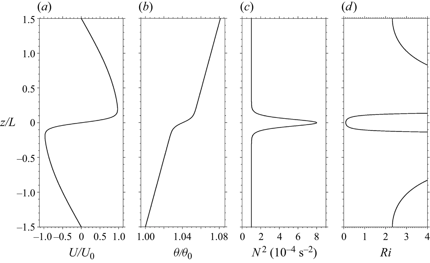


 Open access