


1. Introduction
Turbulent flows in a broad range of natural and engineering applications include small particles, such as water droplets in clouds (Chen et al. Reference Chen, Yau, Bartello and Xue2018), dust particles in protoplanetary disks (Ishihara et al. Reference Ishihara, Kobayashi, Enohata, Umemura and Shiraishi2018) and pneumatic transport of solid particles (Ebrahimi & Crapper Reference Ebrahimi and Crapper2017). These small particles are transported in turbulence and interact with and modify the carrier flow by various processes, having significant results. For example, water droplets in clouds modify the surrounding supersaturation (humidity) field by condensation/evaporation (Grabowski & Wang Reference Grabowski and Wang2013), and small heavy particles in turbulence modify the velocity field of the carrier fluid by the drag force (Elghobashi & Abou-Arab Reference Elghobashi and Abou-Arab1983). These turbulence modulations by small particles crucially affect the subsequent development of the system, such as the fluid mean velocity, heat and mass transfer, dispersion and the growth of particles. Moreover, particles in turbulence lead to many non-trivial phenomena, such as inertial clustering of particles (Sundaram & Collins Reference Sundaram and Collins1997), the sling effect (Falkovich & Pumir Reference Falkovich and Pumir2007) and the clustering of particles in the scalar fronts (Bec, Homann & Krstulovic Reference Bec, Homann and Krstulovic2014). These complex two-way interactions between turbulence and particles, as well as associated phenomena, make it difficult to develop a generally applicable theory or model that can predict the behaviour of particle-laden turbulent flows (Poelma, Westerweel & Ooms Reference Poelma, Westerweel and Ooms2007).
Recently, the development of a model for the particle–turbulence interaction in the research field of cloud turbulence has advanced remarkably (Shaw Reference Shaw2003; Devenish et al. Reference Devenish2012; Grabowski & Wang Reference Grabowski and Wang2013). In the turbulent environment in natural clouds, cloud droplets experience variations in the surrounding supersaturation and velocity field, resulting in different growth histories for cloud droplets by condensation/evaporation and hence broadening of the drop size distributions and acceleration of rain initiation (Sedunov Reference Sedunov1974; Cooper Reference Cooper1989; Korolev & Mazin Reference Korolev and Mazin2003; Lasher-Trapp, Copper & Blyth Reference Lasher-Trapp, Copper and Blyth2005). Two-way interactions between turbulence and cloud droplets by condensation/evaporation are modelled by Langevin-type equations. This Langevin model predicts modulation of the supersaturation field by cloud droplets and broadening of drop-size distributions. The validity and usefulness of the Langevin model have been demonstrated in various studies, including numerical simulations (Sardina et al. Reference Sardina, Picano, Brandt and Caballero2015; Siewert, Bec & Krstulvic Reference Siewert, Bec and Krstulvic2017; Sardina et al. Reference Sardina, Poulain, Brandt and Caballero2018; Saito, Gotoh & Watanabe Reference Saito, Gotoh and Watanabe2019a) and laboratory experiments (Chandrakar et al. Reference Chandrakar, Cantrell, Chang, Ciochetto, Niedermeier, Ovchinnikov, Shaw and Yang2016; Chandrakar, Cantrell & Shaw Reference Chandrakar, Cantrell and Shaw2018; Desai et al. Reference Desai, Chandrakar, Chang, Cantrell and Shaw2018; Chandrakar et al. Reference Chandrakar, Saito, Yang, Cantrell, Gotoh and Shaw2020). In addition, a novel type of cloud microphysics parameterization based on a similar Langevin model was developed in order to take into account the effect of supersaturation fluctuations in unresolved scales on the growth of cloud droplets (Grabowski & Abade Reference Grabowski and Abade2017; Abade, Grabowski & Pawlowska Reference Abade, Grabowski and Pawlowska2018; Thomas, Grabowski & Kumar Reference Thomas, Grabowski and Kumar2020; Chandrakar et al. Reference Chandrakar, Grabowski, Morrison and Bryan2021).
Saito, Watanabe & Gotoh (Reference Saito, Watanabe and Gotoh2019b) considered the case in which the particle–turbulence interaction is due to the drag force. By applying knowledge from cloud turbulence research, they found a new time scale that characterizes turbulence modulation by particles. Based on the results of scaling analysis and direct numerical simulations (DNSs), they demonstrated that turbulence modulation by particles can be expressed as a function of the Damköhler number, which is defined as the ratio of the turbulence large-eddy turnover time to the new time scale.
In order to further extend the study by Saito et al. (Reference Saito, Watanabe and Gotoh2019b), the present study considers the case of thermal coupling, in which particles interact with the fluid temperature field by heat transfer in turbulence. This case has been investigated through numerous DNS studies, a few of which are described below. Bec et al. (Reference Bec, Homann and Krstulovic2014) conducted DNSs of heavy inertial particles transported by a turbulent flow and demonstrated that particles tend to cluster on the fronts of the temperature field, resulting in anomalous scaling laws. Pouransari & Mani (Reference Pouransari and Mani2018) investigated particle-to-fluid heat transfer in particle-laden turbulence for application to particle-based solar receivers (Pouransari & Mani Reference Pouransari and Mani2017; Pouransari et al. Reference Pouransari, Kolla, Chen and Mani2017) and demonstrated the importance of the two dimensionless numbers defined based on a turbulence large-eddy turnover time, i.e. the particle Stokes number and the heat-mixing parameter. They also derived the leading-order thermal evolution equation which reveals the ensemble averaged heat transfer between the particle and fluid phases. Carbone, Bragg & Iovieno (Reference Carbone, Bragg and Iovieno2019) investigated the multiscale aspects of particle–turbulence thermal coupling through statistical analysis, using such as probability density functions and structure functions, and demonstrated the dominance of thermal caustics at small scales, at which the particle temperature differences for small separations rapidly increase as the Stokes number and the thermal Stokes number are increased. However, despite these previous studies, a model or theory that can predict the modulation of fluid temperature fluctuations by particles in turbulence is not yet available.
In order to shed new light on this long-standing problem, we apply the Langevin model used in cloud turbulence research and derive an analytical prediction for modulation of fluid temperature fluctuations by particles. We also conduct DNSs to confirm the theoretical prediction. Being aware of the difficulty in understanding the two-way coupling between particles and turbulence, we here make a step forward by considering the simplest case, in which particles are assumed to be monodisperse, spherical point particles that have finite thermal inertia but have no momentum inertia. In other words, particles move as fluid particles and interact with the surrounding fluid only by thermal coupling. Moreover, no compressibility is considered for a fluid due to temperature change. The fluid is assumed to be incompressible with a constant mass density. Through these simplifications, we can straightforwardly apply the Langevin model to obtain the analytical prediction, which provides a fundamental understanding of the mechanism of the two-way thermal coupling between particles and turbulence.
The remainder of the present paper is organized as follows. Section 2 describes the governing equations. Section 3 provides the theory. Important parameters and non-dimensional numbers are described. The Langevin model used in cloud turbulence research is applied and an analytical prediction for modulation of the temperature fluctuation by particles is derived. In § 4, we describe the DNS of the two-way thermal coupling between particles and turbulence and confirm the theoretical prediction. A summary and discussion are provided in § 5.
2. Governing equations
We consider monodisperse, spherical point particles that have finite thermal inertia but no momentum inertia. Particles move as fluid particles and interact with the surrounding fluid only by thermal coupling. The evolution equations for the particle position are given by
 \begin{equation} \frac{{\textrm{d}}\kern0.06em \boldsymbol{x}_{pj}}{{\textrm{d}}t} = \boldsymbol{u} \left( \boldsymbol{x}_{pj},t \right), \end{equation}
where  $\boldsymbol {x}_{pj}$ is the $j$th particle position, and $\boldsymbol {u}( \boldsymbol {x}_{pj},t )$ is the fluid velocity at $\boldsymbol {x}_{pj}$ at time $t$. The evolution equation for the particle temperature is given by
 \begin{equation} \frac{{\textrm{d}} \theta_{pj}}{{\textrm{d}}t} = \frac{\theta\left( \boldsymbol{x}_{pj},t \right) - \theta_{pj}}{\tau_{\theta}}, \end{equation}
where  $\theta _{pj}$ is the temperature of the $j$th particle, and $\theta ( \boldsymbol {x}_{pj},t )$ is the fluid temperature at $\boldsymbol {x}_{pj}$ at time $t$. In addition, $\tau _{\theta }$ is the particle thermal relaxation time and is given as
 \begin{equation} \tau_{\theta} = \frac{\rho_p c_p r^{2}}{3 \rho_0 c_0 \kappa}, \end{equation}
where  $r$ is the particle radius, $\kappa$ is the thermal diffusivity of the fluid, $\rho _p$ and $\rho _0$ are the particle and fluid densities, respectively, and $c_p$ and $c_0$ are the specific heat capacities of the particle and fluid, respectively, at constant pressure. The thermal equations for particles (2.2) and (2.3) are based on solutions for spherical particles in an infinite domain.
The fluid is assumed to be incompressible with a constant mass density. In order to focus on the thermal coupling, the feedback effect from the particles to the fluid is considered only for the fluid temperature and not for the fluid velocity. The velocity field of a fluid is governed by the incompressible Navier–Stokes equations,
 \begin{align} \frac{\partial \boldsymbol{u}}{\partial t } + \boldsymbol{u}\boldsymbol{\cdot}\boldsymbol{\nabla} \boldsymbol{u} &={-} \frac{\boldsymbol{\nabla} p}{\rho_0} + \nu \nabla^{2} \boldsymbol{u} + \boldsymbol{f}_{\boldsymbol{u}}, \end{align}
 \begin{align} \boldsymbol{\nabla}\boldsymbol{\cdot} \boldsymbol{u} &= 0, \end{align}
where  $p$ is the pressure and $\boldsymbol {f}_{\boldsymbol {u}}$ represents the external force, which is solenoidal ( $\boldsymbol {\nabla } \boldsymbol {\cdot } \boldsymbol {f}_{\boldsymbol {u}} = 0$). The temperature field for the fluid is governed by the advection–diffusion equation,
 \begin{equation} \frac{\partial \theta }{ \partial t } + \boldsymbol{u}\boldsymbol{\cdot}\boldsymbol{\nabla} \theta = \kappa \nabla^{2} \theta + F_p + f_{\theta}, \end{equation}
where  $f_{\theta }$ represents the external force. Here, $F_p$ is the feedback term from particles due to two-way thermal coupling,
 \begin{equation} F_p ={-} \frac{1}{\rho_0 c_0} \sum_{j=1}^{N_p} c_p m_p \left[\frac{\theta\left(\boldsymbol{x}_{pj} \right) - \theta_{pj} }{\tau_{\theta}} \right] \delta(\boldsymbol{x}-\boldsymbol{x}_{pj}), \end{equation}
where  $N_p$ is the total number of particles in the domain, $m_p = 4 \rho _p {\rm \pi}r^{3} / 3$ is the particle mass and $\delta ()$ is the Dirac delta function.
Note that, since the temperature equations (2.6) and (2.7) are linear for both  $\theta$ and $\theta _{pj}$, we can regard $\theta$ and $\theta _{pj}$ as deviations from a constant reference temperature $T_{ref}$. Namely, actual fluid and particle temperatures are given by $(\theta + T_{ref})$ and $(\theta _{pj} + T_{ref})$, respectively, and $T_{ref}$ is set so that $\langle \theta \rangle =0$ in a statistically steady state of turbulence, where the angle brackets indicate an ensemble average over turbulence realizations.
3. Theory
3.1. Characteristic time scales and non-dimensional numbers
The characteristic response time of the particle temperature to the surrounding fluid temperature field is given by the particle thermal relaxation time  $\tau _{\theta }$ in (2.3). On the other hand, the characteristic response time of the fluid temperature field to the temperature of suspended particles is given by the fluid thermal relaxation time,
 \begin{equation} \tau_{\theta f} = (4 {\rm \pi}\kappa n_p r)^{{-}1},\end{equation}
where  $n_p$ is the particle number density ( $\tau _{\theta f}$ is referred to as the ‘gas thermal relaxation time’ in Pouransari & Mani (Reference Pouransari and Mani2018)). Here, $\tau _{\theta f}$ is inversely proportional to the particle number density $n_p$ and the particle radius $r$. This formula is similar to that for the phase relaxation time, an important time scale in cloud physics that characterizes the particle–turbulence interaction by condensation/evaporation (Politovich & Cooper Reference Politovich and Cooper1988; Korolev & Mazin Reference Korolev and Mazin2003; Kostinski Reference Kostinski2009). Recently, a time scale of similar form was found for the particle–turbulence interaction by the drag force (Saito et al. Reference Saito, Watanabe and Gotoh2019b).
There are three important non-dimensional numbers that characterize the two-way thermal interaction between particles and fluid. First, the particle-to-fluid heat capacity ratio is expressed as the ratio of  $\tau _{\theta }$ to $\tau _{\theta f}$ as
 \begin{equation} \phi_{\theta} = \frac{C_p}{C_0} = \frac{c_p \phi_m}{c_0} = \frac{\tau_{\theta}}{\tau_{\theta f}}, \end{equation}
where  $C_0$ and $C_p$ are the heat capacities of fluid and particles in the domain, respectively, $\phi _m$ is the mass-loading parameter given as
 \begin{equation} \phi_m = \frac{\rho_p \phi_v}{\rho_0} = \frac{\rho_p n_p (4 {\rm \pi}r^{3} /3)}{\rho_0}, \end{equation}
and  $\phi _v$ is the volume fraction. Second, the ratio of $T$ to $\tau _{\theta f}$, where $T$ is the large-eddy turnover time for the turbulent velocity field, is represented by the Damköhler number as
 \begin{equation} Da = \frac{T}{\tau_{\theta f}}. \end{equation}
Here,  $T={\mathcal {L}}/u_{rms}$ where ${\mathcal {L}}$ is the integral scale and $u_{rms}$ is the root-mean-square velocity (see Appendix D for definitions of other turbulence parameters). Third, the ratio of $\tau _{\theta }$ to $T$ is represented by the thermal Stokes number for the large-scale flow as
 \begin{equation} St_{L} = \frac{\tau_{\theta}}{T}, \end{equation}
where the subscript  $L$ indicates that $St_{L}$ is that for the large-scale eddies of turbulent flow. From (3.4) and (3.5), $\phi _{\theta }$ is also expressed by $Da$ and $St_L$ as
 \begin{equation} \phi_{\theta} = Da St_L. \end{equation}
 Note that the large-eddy turnover time,  $T$, is used in the definitions of (3.4) and (3.5) because the largest eddies are considered to be the most important in the thermal coupling. This conjecture was first proposed for the particle–turbulence interaction by condensation/evaporation and was confirmed by DNSs of cloud turbulence (Lanotte, Seminara & Toschi Reference Lanotte, Seminara and Toschi2009; Sardina et al. Reference Sardina, Picano, Brandt and Caballero2015; Götzfried et al. Reference Götzfried, Kumar, Shaw and Schumacher2017; Kumar et al. Reference Kumar, Götzfried, Suresh, Schumacher and Shaw2018; Saito et al. Reference Saito, Gotoh and Watanabe2019a). Later this assumption was shown to also hold for the particle–turbulence interaction by the drag force (Saito et al. Reference Saito, Watanabe and Gotoh2019b). Note also that the importance of the Damköhler number was recently demonstrated by Pouransari & Mani (Reference Pouransari and Mani2018) for the particle-to-fluid heat transfer in particle-laden turbulence. They referred to the inverse of the Damköhler number ( $Da^{-1} = \tau _{\theta f}/T$) as the heat-mixing parameter, as opposed to the commonly used heat-mixing parameter defined using the particle thermal relaxation time $\tau _{\theta }$. In the present study, we use the term ‘Damköhler number’ for (3.4) in order to emphasize the relation with cloud-turbulence research. Originally, the Damköhler number came from chemical engineering and described the ratio of the turbulent flow time scale and the chemical reaction time scale (Dimotakis Reference Dimotakis2005). In the cloud physics literature, a similar parameter was introduced to examine the role of cloud entrainment and turbulent mixing in the growth of cloud droplets by condensation/evaporation. Since the growth of cloud droplets has some similarities to a chemical reaction, the Damköhler number term has been used (Shaw Reference Shaw2003; Devenish et al. Reference Devenish2012). Saito et al. (Reference Saito, Watanabe and Gotoh2019b) introduced another similar parameter for momentum coupling and referred to it also as the Damköhler number. In order to distinguish a variety of Damköhler numbers, it is useful to add an additional adjective before it, for example: the supersaturation Damköhler number for cloud physics (as used by Shaw Reference Shaw2003); the inertial Damköhler number for momentum coupling; the thermal Damköhler number for (3.4). In the present study, however, we simply refer to (3.4) as the Damköhler number, for brevity.
3.2. Modulation of fluid temperature fluctuations by particles
We apply the Langevin model in order to derive the analytical expression for modulation of fluid temperature fluctuations by particles. We assume that turbulence is statistically homogeneous, is in a statistically steady state and is excited by the external forces  $\boldsymbol {f}_{\boldsymbol {u}}$ and $f_{\theta }$ in (2.4) and (2.6), respectively, that are Gaussian random, white in time and homogeneous isotropic. We also assume that, both in cases with and without particles, the injection rate of the temperature-fluctuation variance is kept at $\chi _0$.
For cloud turbulence, the Langevin equation models the time variation of the supersaturation along the Lagrangian trajectory of cloud droplets. The feedback effect from cloud droplets on the supersaturation field is expressed by the term with the phase relaxation time  $\tau _c$, and the turbulent mixing is expressed by the term with the large-eddy turnover time $T$. (For more details, readers are referred to, for example, Chandrakar et al. (Reference Chandrakar, Cantrell, Chang, Ciochetto, Niedermeier, Ovchinnikov, Shaw and Yang2016).) In the present system, i.e. (2.1) to (2.7), the fluid temperature $\theta$ corresponds to the supersaturation, and the fluid thermal relaxation time $\tau _{\theta f}$ corresponds to $\tau _c$. Therefore, the Langevin model can be straightforwardly applied to the present system.
The situation under consideration is as follows. The number density of particles is  $n_p$ and particles are uniformly randomly distributed in the domain. As described in Saito et al. (Reference Saito, Watanabe and Gotoh2019b), we divide the domain into small subdomains and assume that each subdomain includes only a single particle (Tagawa et al. Reference Tagawa, Mercado, Prakash, Calzavarini, Sun and Lohse2012). The volume of the subdomain can be estimated approximately as $1/n_p$. The particle number density $n_p$ is assumed to be sufficiently large so that the characteristic length of the subdomain is smaller than the smallest length scale of the fluid temperature fluctuation (the Batchelor scale $\eta _{B}$) and that the fluid temperature in the subdomain can be regarded as uniform. In the subdomain, the fluid temperature is $\theta$ and the particle temperature is $\theta _p$. As time goes on, the fluid in the subdomain is advected by the turbulent velocity field as a small Lagrangian fluid parcel. Since we neglect the momentum inertia of the particle, the particle moves in the same way as the surrounding fluid parcel. From (2.6), the evolution equation for the temperature of the Lagrangian fluid parcel, $\theta$, is modelled by the Langevin equation as follows:
 \begin{equation} \theta(t+{\textrm{d}}t) - \theta(t) ={-} \alpha c \left( \frac{\theta - \theta_p}{\tau_{\theta f}} \right){\textrm{d}}t - \alpha \left( \frac{\theta}{T} \right){\textrm{d}}t + \alpha \left( \frac{2 \theta_0^{2} \,{\textrm{d}}t}{T} \right)^{1/2} \eta(t), \end{equation}
where  $\theta _0$ is the standard deviation of the fluid temperature fluctuation without the effect of particles, $\eta (t)$ is a Gaussian random number with zero mean and unit variance which is statistically independent of $\theta$ and $\theta _p$, and $\alpha$ and $c$ are constants that are determined depending on the actual situation of the turbulence. The equation for the particle temperature is the same as (2.2), i.e.
 \begin{equation} \frac{{\textrm{d}} \theta_p}{{\textrm{d}}t} = \frac{\theta - \theta_p}{\tau_{\theta}}. \end{equation}
Since (3.7) and (3.8) are linear in  $\theta$ and $\theta _p$, we can derive the analytical expressions for the statistically steady state.
We first consider the particle temperature  $\theta _p$. Multiplying (3.8) by $\theta _p$ and taking an average, we have
 \begin{equation} \frac{{\textrm{d}}}{{\textrm{d}}t}\left( \frac{1}{2} \langle \theta_p^{2} \rangle_{p} \right) = \frac{1}{\tau_{\theta}} ( \langle \theta \theta_p \rangle_{p} - \langle \theta_p^{2} \rangle_{p}), \end{equation}
where  $\langle \, \rangle _{p}$ indicates an average over particles. Since the left-hand side is zero in a statistically steady state, we have
 \begin{equation} \langle \theta \theta_p \rangle_{p} = \langle \theta_p^{2} \rangle_{p}. \end{equation}
Multiplying (3.7) by  $\theta _p$ and taking an average $\langle \, \rangle _{p}$, we have
 \begin{equation} \left\langle \theta_p \frac{{\textrm{d}} \theta}{{\textrm{d}}t} \right\rangle_{p} ={-} \alpha \left( \frac{ \langle \theta \theta_p \rangle_{p} }{T} \right), \end{equation}
since the feedback terms from particles cancel out due to (3.10) and  $\langle \eta (t) \theta _p \rangle _{p} =0$. Multiplying (3.8) by $\theta$ and taking an average $\langle \, \rangle _{p}$, we have
 \begin{equation} \left\langle \theta \frac{{\textrm{d}} \theta_p}{{\textrm{d}}t} \right\rangle_{p} = \frac{ \langle \theta^{2} \rangle - \langle \theta \theta_p \rangle_{p} }{\tau_{\theta}}. \end{equation}
Summing (3.11) and (3.12), we obtain
 \begin{equation} \frac{{\textrm{d}}}{{\textrm{d}}t}\left( \frac{1}{2} \langle \theta \theta_p \rangle_{p} \right) ={-} \alpha \left( \frac{ \langle \theta \theta_p \rangle_{p} }{T} \right) + \frac{1}{\tau_{\theta}} (\langle \theta^{2} \rangle - \langle \theta \theta_p \rangle_{p} ). \end{equation}
In a statistically steady state, we have
 \begin{equation} \langle \theta \theta_p \rangle_{p} = \left( \frac{\alpha}{T} + \frac{1}{\tau_{\theta}} \right)^{{-}1} \frac{\langle \theta^{2} \rangle_{p} }{\tau_{\theta}}. \end{equation}
Combining (3.10) and (3.14) and using the definition of (3.5), we finally obtain
 \begin{equation} \frac{ \langle \theta_p^{2} \rangle_{p} }{ \langle \theta^{2} \rangle_{p} } = \left( 1 + \alpha St_L \right)^{{-}1}. \end{equation}
This equation predicts the variance ratio of the fluctuations of particle and fluid temperatures.
We next consider the fluid temperature  $\theta$. Here, we consider the dissipation of the temperature fluctuation variance. Since the injection rate is kept at a constant $\chi _0$ with or without particles, for the case without particles, we have
 \begin{equation} \chi_0 \sim \frac{\alpha}{T} \theta_0^{2} \end{equation}
and, for the case with particles, we have
 \begin{equation} \chi_0 \sim \frac{\alpha}{T} \langle \theta^{2} \rangle_{p} + \frac{\alpha c}{\tau_{\theta f}} ( \langle \theta^{2} \rangle_{p} - \langle \theta \theta_p \rangle_{p} ) \end{equation}
using (3.7). Equating (3.16) and (3.17) yields
 \begin{equation} \frac{\alpha}{T} \theta_0^{2} = \frac{\alpha}{T} \langle \theta^{2} \rangle_{p} + \frac{\alpha c}{\tau_{\theta f}} (\langle \theta^{2} \rangle_{p} - \langle \theta \theta_p \rangle_{p}). \end{equation}
Substituting (3.10) and (3.15) into the above equation and using the definitions of (3.2)–(3.6), we finally obtain
 \begin{equation} \frac{\langle \theta^{2} \rangle_{p}}{\theta_0^{2}} = \left( 1+ \frac{ c \alpha \phi_{\theta}}{1+ \alpha \phi_{\theta} Da^{{-}1}} \right)^{{-}1}. \end{equation}
This equation predicts modulation of the fluid temperature fluctuation variance by particles as a function of the Damköhler number.
We consider two limits of (3.19). First, for the limit  $Da \rightarrow 0$ with fixed $\phi _{\theta }$, we have
 \begin{equation} \frac{\langle \theta^{2} \rangle_{p}}{\theta_0^{2}} \rightarrow \left( 1 + c Da \right)^{{-}1} \quad (Da \rightarrow 0). \end{equation}
Second, for the limit  $Da \rightarrow \infty$ with fixed $\phi _{\theta }$, we have
 \begin{equation} \frac{\langle \theta^{2} \rangle_{p}}{\theta_0^{2}} \rightarrow \left( 1 + c \alpha \phi_{\theta} \right)^{{-}1} \quad (Da \rightarrow \infty), \end{equation}
which indicates that modulation of the variance approaches a constant depending on  $\phi _{\theta }$.
In summary, in a statistically steady state, (3.15) predicts the variance ratio of the particle and fluid temperature fluctuations, and (3.19) predicts modulation of the fluid temperature fluctuation variance by particles.
3.2.1. Modulation by particles with fixed temperature
An important limit case of the Langevin model given by (3.7) and (3.8) is the case in which the particle temperature fluctuation  $\theta _p$ is fixed at zero. This physically corresponds to particles with large thermal inertia ( $St_L \rightarrow \infty$). In this case, the Langevin model reduces to
 \begin{equation} \theta(t+{\textrm{d}}t) - \theta(t) ={-} \alpha c \left( \frac{\theta}{\tau_{\theta f}} \right){\textrm{d}}t - \alpha \left( \frac{\theta}{T} \right){\textrm{d}}t + \alpha \left( \frac{2 \theta_0^{2} \,{\textrm{d}}t}{T} \right)^{1/2} \eta(t),\end{equation}
which is equivalent to the Langevin model used in cloud turbulence research (except for constants  $c$ and $\alpha$ – see (2) in Chandrakar et al. (Reference Chandrakar, Cantrell, Chang, Ciochetto, Niedermeier, Ovchinnikov, Shaw and Yang2016)). In a statistically steady state, we obtain the same result as (3.20), which is the same formula as (3) in Chandrakar et al. (Reference Chandrakar, Cantrell, Chang, Ciochetto, Niedermeier, Ovchinnikov, Shaw and Yang2016).
3.2.2. Particle temperature fluctuation for the one-way coupling case
Another important limit case of the Langevin model (3.7) and (3.8) is the case without the feedback effect of particles on the fluid temperature field, namely, the one-way coupling case. In this case, (3.7) reduces to
 \begin{equation} \theta(t+{\textrm{d}}t) - \theta(t) ={-} \alpha \left( \frac{\theta}{T} \right){\textrm{d}}t + \alpha \left( \frac{2 \theta_0^{2} \,{\textrm{d}}t}{T} \right)^{1/2} \eta(t), \end{equation}
and the equation for the particle temperature is the same as (3.8), as follows:
 \begin{equation} \frac{{\textrm{d}} \theta_p}{{\textrm{d}}t} = \frac{\theta - \theta_p}{\tau_{\theta}}.\end{equation}
In a statistically steady state, we obtain the same result as (3.15) for the particle temperature, as follows:
 \begin{equation} \frac{ \langle \theta_p^{2} \rangle_{p} }{ \langle \theta^{2} \rangle_{p} } = \left( 1 + \alpha St_L \right)^{{-}1}, \end{equation}
whereas  $\langle \theta ^{2} \rangle _{p} = \theta _0^{2}$ for the fluid temperature because the coupling is one-way. Note that a relationship similar to (3.25) was recently derived by Carbone et al. (Reference Carbone, Bragg and Iovieno2019) (see their (4.5)).
4. DNS
4.1. Simulation set-up
In order to confirm the theoretical prediction obtained in the previous section, we conduct DNS of particles in turbulence using the cloud microphysics simulator, which is a DNS model developed for the large-scale computation of particle-laden turbulent flow (Gotoh, Suehiro & Saito Reference Gotoh, Suehiro and Saito2016; Saito & Gotoh Reference Saito and Gotoh2018). The numerical domain is a periodic cubic box with a length  $L_{box}$ per side. Particles are regarded as spherical point particles. The fluid velocity and temperature at the particle position, $\boldsymbol {u} (\boldsymbol {x}_{pj} )$ and $\theta (\boldsymbol {x}_{pj})$, are calculated from the velocity and temperature fields at the surrounding eight grid points by linear interpolation, respectively. The same weighting is used to project the particle temperature, $\theta _{pj}$, onto the surrounding eight grid points to calculate the term $F_p$ in (2.7), i.e. the particle-in-cell method (Sundaram & Collins Reference Sundaram and Collins1996).
We numerically integrate the evolution equations (2.1), (2.2), (2.4) and (2.6) using the second-order Runge–Kutta scheme and the pseudospectral method for temporal and spatial discretization, respectively. The external forces  $\boldsymbol {f}_{\boldsymbol {u}}$ and $f_{\theta }$ in (2.4) and (2.6) are homogeneous isotropic, applied to all wavenumber components within a shell of $1 \leq k L_{box} \leq 4$, and are produced by Gaussian random, white-in-time processes (Gotoh, Fukuyama & Nakano Reference Gotoh, Fukuyama and Nakano2002). The details of the external forces are provided in Appendix A. These simple forces are enough for the fundamental study. After a statistically steady state is achieved for each simulation, turbulence and particle statistics are calculated.
Numerical and physical parameters in the present DNS are summarized in table 1. We studied five values of the total grid number ( $N_{grid}^{3}=32^{3}$– $512^{3}$) and 10 values of the particle radius ( $r=1.0$– $1000\,\mathrm {\mu }$m). The total number of particles $N_p$ is set equal to the total grid number $N_{grid}^{3}$, corresponding to the particle number density $n_p = 125$ cm $^{-3}$. For the particle-to-fluid heat capacity ratio, we chose three values ( $\phi _{\theta }=1.0$, $0.3$ and $0.1$) and conducted two additional simulations. In one simulation, the particle temperature was fixed at zero ( $\theta _{pj}=0$) and, in the other simulation, the thermal coupling was one-way (the feedback from particles onto the fluid was neglected). In total, we conducted $5 \times 10 \times (3+2)=250$ kinds of simulations. Table 2 summarizes the particle radius $r$, the fluid thermal relaxation time $\tau _{\theta f}$, the volume fraction $\phi _v$ and the particle-to-fluid density ratio $\rho _p/\rho _0$ for each simulation.
Table 1. Various numerical and physical parameters. The time step is  $\Delta t = 1.0 \times 10^{-3}$ (s) for simulations with $N_{grid}=32$, $64$,
$64$,  $128$, and $256$ and is $\Delta t = 8.0 \times 10^{-4}$ (s) for simulations with $N_{grid}=512$. The box length is $L_{box}=N_{grid} \Delta x$. The total number of particles is $N_p= n_p L_{box}^{3} =N_{grid}^{3}$. The density of particles is $\rho _p=(3 \rho _0 c_0 \phi _{\theta })/(4 {\rm \pi}n_p c_p r^{3})$. For parameter $\phi _{\theta }$, ‘1.0 (one-way)’ indicates simulations with $\phi _{\theta }=1$ and one-way thermal coupling, and ‘ $\theta _p$ zero’ indicates simulations with the particle temperature fixed at zero.

Table 2. Particle parameters. Here,  $r$ is the particle radius, $\tau _{\theta f}$ is the fluid thermal relaxation time and $\phi _v$ is the volume fraction. The particle-to-fluid density ratio ( $\rho _p/\rho _0$, as determined by (3.2) and (3.3)) is listed for simulations with $\phi _{\theta }=1.0$, $0.3$ and $0.1$. The particle thermal relaxation time is given by $\tau _{\theta }=\phi _{\theta } \tau _{\theta f}$ ( $\phi _{\theta }=1.0, 0.3, 0.1$).

In table 1, the values of  $c_0$ and $c_p$ are taken from Saito et al. (Reference Saito, Gotoh and Watanabe2019a) and Sato, Deutsch & Simonin (Reference Sato, Deutsch and Simonin1998), respectively. From (3.2), the mass-loading parameters corresponding to $\phi _{\theta }=1.0$, $0.3$ and $0.1$ are $\phi _m = 2.6$, $0.78$ and $0.26$, respectively. Although $\phi _m$ is an important parameter for turbulence modulation by particles due to the drag force (Squires & Eaton Reference Squires and Eaton1993; Saito et al. Reference Saito, Watanabe and Gotoh2019b), $\phi _m$ is not important in the present study because momentum coupling is neglected and the particles move as fluid particles.
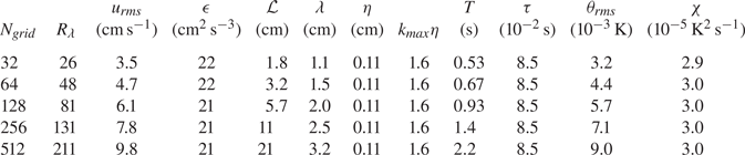
The important premise in the Langevin model in the previous section is that the largest eddies play the central role in the particle–turbulence interaction by the two-way thermal coupling. We check the validity of this premise using the same strategy as that used by Lanotte et al. (Reference Lanotte, Seminara and Toschi2009) (see also Saito et al. (Reference Saito, Watanabe and Gotoh2019b)). Namely, we fix the turbulence statistics for the smallest eddies and expand the number of grids, the domain size and the sizes of the largest eddies in order to investigate the interaction between the largest eddies and particles. Turbulence statistics without particles are summarized in table 3. Note that fluid temperature statistics are modulated by the effect of particles.
Table 3. Mean turbulence parameters for cases without particles. Here,  $N_{grid}$ is the number of grid points in physical space for each direction, $R_{\lambda }$ is the Taylor microscale Reynolds number, $u_{rms}$ is the root-mean-square velocity, $\epsilon$ is the mean energy dissipation rate per unit mass, $\mathcal {L}$ is the integral scale, $\lambda$ is the Taylor microscale, $\eta$ is the Kolmogorov length, $k_{max}\eta$ is the cutoff wavenumber normalized by the Kolmogorov length, $T$ is the large-eddy turnover time, $\tau$ is the Kolmogorov time, $\theta _{rms}$ is the root-mean-square temperature fluctuation ( $=\theta _0$ in (3.7)) and $\chi$ is the mean dissipation rate for the temperature variance. See Appendix D for definitions of turbulence parameters.
In the present study, the system is characterized by five independent non-dimensional numbers: the Taylor microscale Reynolds number  $Re_{\lambda }$; the Prandtl number $Pr=\nu /\kappa$ which is unity; the particle-to-fluid heat capacity ratio $\phi _{\theta } = \tau _{\theta }/\tau _{\theta f}$; the Damköhler number $Da = T/\tau _{\theta f}$ (or the thermal Stokes number for lerge scale flow $St_L = \tau _{\theta }/T$); and the thermal Stokes number defined by the Kolmogorov time, $St_{\theta }=\tau _{\theta }/\tau$, where $\tau$ is the Kolmogorov time. Either $Da$ or $St_L$ can be removed by (3.6).
For all of the following simulation results, we confirmed that  $\langle \theta ^{2} \rangle _p$ is almost identical to $\langle \theta ^{2} \rangle _V$, where $\langle \, \rangle _V$ indicates the volume average (agreement is better for simulations with larger $N_{grid}$ and $N_p$, ranging from 97.1 % for $N_{grid}=32$ to 99.6 % for $N_{grid}=512$). In other words, the variance of the fluid temperature fluctuation does not change whether the average is taken over particles or over grid points. This is because the total number of particles $N_p$ is sufficiently large (same as the total grid number) and particles are almost uniformly randomly distributed in the domain in the present simulation. We also confirmed that the probability density functions of both the fluid and particle temperature fluctuations are all Gaussian.
4.2. Results
4.2.1. Two limiting cases
We first investigate the results for the simulations in which the particle temperature is fixed at zero ( $\theta _{pj}=0$). Figure 1(a) shows the ratio $\langle \theta ^{2} \rangle _{p}/\theta _0^{2}$, where $\theta _0^{2}$ and $\langle \theta ^{2} \rangle _{p}$ are the variances of fluid temperature fluctuations without and with the effect of particles, respectively. The horizontal axis is $Da$, i.e. the Damköhler number in (3.4). The orange curve indicates the theoretical prediction (3.20) with $c=1.59$ ( $c$ is estimated by curve-fitting method). All of the simulation results collapse nicely onto the theoretical curve. The slope of the curve is close to $-1$ for $Da > 1$, indicating that the scalar energy injected by the external force is dissipated mainly by particles in this range.

Figure 1. (a) Ratio  $\langle \theta ^{2} \rangle _{p} / \theta _0^{2}$ for the cases with the particle temperature fixed at zero ( $\theta _{pj}=0$), where $\langle \theta ^{2} \rangle _{p}$ and $\theta _0^{2}$ are the variances of the fluid temperature fluctuations with and without particles, respectively. The horizontal axis is the Damköhler number $Da = T/\tau _{\theta f}$. The orange curve indicates the theoretical prediction (3.20) with $c=1.59$. The short black line indicates a slope of $-1$, which is expected for $Da \gg 1$ from (3.20). (b) Ratio $\langle \theta _p^{2} \rangle _{p} / \langle \theta ^{2} \rangle _{p}$ for the cases with one-way thermal coupling, where $\langle \theta _p^{2} \rangle _{p}$ is the fluctuation variance of the particle temperature. The horizontal axis is the thermal Stokes number for the large-scale flow $St_L = \tau _{\theta }/T$. The orange curve indicates the theoretical prediction (3.25) with $\alpha =1.31$. The short black line indicates the slope of $-1$ expected for $St_L \gg 1$ from (3.25). Note that $\langle \theta ^{2} \rangle _{p} = \theta _0^{2}$ for the one-way coupling case.
We next investigate the results for the simulations with one-way thermal coupling. Figure 1(b) shows the ratio  $\langle \theta _p^{2} \rangle _{p} /\langle \theta ^{2} \rangle _{p}$, where $\langle \theta _p^{2} \rangle _{p}$ is the fluctuation variance of the particle temperature. Note that $\langle \theta ^{2} \rangle _{p} = \theta _0^{2}$ for the one-way coupling case. The horizontal axis is $St_L$, which is the thermal Stokes number in terms of the large-scale flow in (3.5). The orange curve indicates the theoretical prediction (3.25) with $\alpha =1.31$ ( $\alpha$ is estimated by a curve-fitting method). Again, all of the simulation results collapse nicely onto the theoretical curve.
4.2.2. Two-way coupling cases
Now, we investigate the simulation results for the two-way thermal coupling case. The theoretical prediction (3.15) indicates that the variance ratio of the particle and fluid temperature fluctuations,  $\langle \theta _p^{2} \rangle _{p} /\langle \theta ^{2} \rangle _{p}$, is the same as that for the one-way coupling case (3.25). This is confirmed by figures 2(a) to 2(c), which summarize $\langle \theta _p^{2} \rangle _{p} /\langle \theta ^{2} \rangle _{p}$ for the simulations with $\phi _{\theta }=1$, $0.3$ and $0.1$, respectively. The orange curve indicates the theoretical curve (3.15) with the same value of $\alpha$ as in figure 1(b). Although there is slight dependence on the Reynolds number $R_{\lambda }$ (or the number of grids $N_{grid}$) and the heat capacity ratio $\phi _{\theta }$, all of the simulation results collapse onto the theoretical curve fairly well.

Figure 2. Same as figure 1(b), except that the particle temperature is not fixed and the particle-to-fluid heat capacity ratios are  $\phi _{\theta }=1$, $0.3$ and $0.1$ for (a–c), respectively. Note that the vertical axis is linear and the horizontal axis is from $10^{-3}$.
Figures 3(a) to 3(c) summarize the ratio  $\langle \theta ^{2} \rangle _{p} /\theta _0^{2}$, or the modulation of the fluid temperature variance by particles, based on the simulation results for the two-way coupling case with $\phi _{\theta }=1$, $0.3$ and $0.1$, respectively. For each panel, all simulation results collapse onto the theoretical curve (dashed grey curve) fairly well. The theoretical curve (dashed grey curve) follows the curve for the fixed-particle-temperature case (orange curve) for $Da < \phi _{\theta }$ (as shown in (3.20)) and starts to deviate from the fixed-particle-temperature case for $Da \sim \phi _{\theta }$ and approaches a value of $( 1 + c \alpha \phi _{\theta } )^{-1}$, which is independent of $Da$ for $Da > \phi _{\theta }$ (as shown in (3.21)).

Figure 3. Same as figure 1(a), except that the particle temperature is not fixed and the particle-to-fluid heat capacity ratios are  $\phi _{\theta }=1$, $0.3$ and $0.1$ for (a–c), respectively. The dashed grey curve indicates the theoretical prediction (3.19) with $c=1.59$ and $\alpha =1.31$. The solid orange curve indicates the theoretical prediction (3.20) with $c=1.59$. Note that the vertical axis is linear.
The physical interpretation of the results in figure 3 is as follows. For  $Da < \phi _{\theta }$, $St_L > 1$ and $\tau _{\theta } > T$ from (3.4)–(3.6). The particle thermal relaxation time $\tau _{\theta }$ is greater than the large-eddy turnover time $T$, and the particle temperature responds only slowly to the change in the surrounding fluid temperature field due to turbulent mixing. As a result, the particle temperature does not deviate from the reference temperature so much, and the variance $\langle \theta _p^{2} \rangle _{p}$ is small in comparison with the fluid temperature variance $\langle \theta ^{2} \rangle _{p}$ (as shown in figure 2 for $St_L>1$). Therefore, modulation of the fluid temperature variance by particles is close to that for the case with a fixed particle temperature (orange curves in figure 3, see (3.20)). On the other hand, for $Da > \phi _{\theta }$, $St_L < 1$ and $\tau _{\theta } < T$. The particle temperature responds increasingly quickly to the change in the surrounding fluid temperature, and the temperature difference between the fluid and particles decreases. As a result, modulation of the fluid temperature variance by particles is limited and smaller than the case with a fixed particle temperature (see (3.21)).
We emphasize the importance of using  $Da$ and $St_L$, both of which include the large-eddy turnover time $T$ in their definitions, in order to obtain the good collapse of the simulation results in figures 1–3. Such a good collapse cannot be obtained if we use a non-dimensional number defined with the Kolmogorov time $\tau$. This is confirmed in Appendix B, where the thermal Stokes number $St_{\theta }=\tau _{\theta }/\tau$ is used as an example. These results support that the largest eddies play the most important role in modulation of the fluid and particle temperature variances.
Before closing this section, we briefly mention the time evolution and spatial distribution of fluctuations. Although the main focus of the present study is on the steady-state values of the fluid and particle temperature variances, we also took data of time evolution and spatial distribution of fluctuations. Some typical results are provided in Appendix C for the case with  $N_{grid}=512$, $\phi _{\theta }=1$ and $r=20\,\mathrm {\mu }$m.
5. Summary and discussion
In the present study, we investigated modulation of the fluid temperature fluctuations by particles due to thermal interaction in homogeneous isotropic turbulence. For the benefit of simplicity, only thermal coupling between the fluid and particle was considered, and momentum coupling was neglected. Particles were assumed to move as fluid particles and interact with the surrounding fluid only by heat transfer. Moreover, the fluid is assumed to be incompressible and to have a constant mass density. By virtue of these simplifications, we straightforwardly applied the Langevin model used in cloud turbulence research and obtained an analytical prediction for modulation of the intensity of the fluid temperature fluctuations by particles as a function of the Damköhler number, which is defined as the ratio of the turbulence large-eddy turnover time to the fluid thermal relaxation time. We also conducted DNS of the two-way thermal coupling between particles and turbulence and confirmed that the simulation results agree well with the theoretical predictions.
Modulation of fluid temperature fluctuations by particles due to heat transfer obtained in the present study is qualitatively very similar to turbulence modulation by particles due to the drag force obtained by DNS in Saito et al. (Reference Saito, Watanabe and Gotoh2019b) (compare their figure 3 with our figure 3). It should also be noted that, while Saito et al. (Reference Saito, Watanabe and Gotoh2019b) considered momentum coupling and hence included the effects of inertial clustering and associated phenomena, the present study does not include those effects since momentum coupling is neglected and particles are almost uniformly randomly distributed in the domain. Despite this difference, we obtained very similar results. This similarity strongly suggests that turbulence modulation due to momentum and thermal couplings share a similar underlying mechanism and also that the Langevin model used in cloud turbulence research should be a useful tool for clarification of turbulence modulation by particles. Since a theoretical prediction of modulation (such as (3.21)) has not yet been achieved for the case of the drag force, the application of the Langevin model might be a promising method. This possibility will be explored in a future study.
Since the present study assumed several simplifications of the particle–turbulence interaction, the interpretation of the present results needs some care. Especially, since particle momentum and thermal relaxation times are usually similar in natural and engineering applications, it is important to include momentum coupling. In such a case, the fluid velocity field is also modulated by particles due to the drag force, and the large-eddy turnover time  $T$ can no longer be taken as a constant parameter in the Langevin model. In addition, due to the momentum inertia of the particle, the trajectory of the particle deviates from that of the Lagrangian fluid particle. As a preliminary test, we conducted several additional simulations in Appendix E in order to investigate the effect of momentum coupling on modulation of fluid temperature fluctuations. The set-up is the same as that for DNSs with $N_{grid}=128$ and $\phi _{\theta }=0.1$ in § 4, except that either one- or two-way momentum coupling is included. For the one-way momentum coupling case, modulation of the fluid temperature variance is almost unchanged as compared with the case without momentum inertia. On the other hand, for the two-way momentum coupling case, the fluid temperature variance is significantly increased by particles as compared with the case without momentum inertia. However, this is only due to attenuation of turbulent kinetic energy by particles which in turn leads to the increase in the large-eddy turn over time, and not due to the effects of inertial clustering and associated phenomena. Appendix E also confirms that the theoretical prediction (3.19) is still useful for the study of cases with momentum coupling. Clearly, more comprehensive simulations are required to be conclusive, but this is left as future work.
Another important task is to clarify the effect of the forcing mechanism used for the injection of kinetic energy and scalar variance in DNS. Although the present DNS used a Gaussian white-in-time random force both for velocity and scalar fields, many other forcing mechanisms have been proposed and one of them is the forcing based on a uniform mean scalar gradient:  $f_{\theta }= \varGamma u_3$, where $u_3$ is the vertical component of ${\boldsymbol u}$ and $\varGamma$ is a constant. This form is commonly used in DNSs of passive scalars (Gotoh & Watanabe (Reference Gotoh and Watanabe2015), Yasuda et al. (Reference Yasuda, Gotoh, Watanabe and Saito2020) and references therein) and is also relevant to cloud physics where the temperature and supersaturation fluctuations are excited by the vertical air motion in the stratified environment (Thomas et al. Reference Thomas, Grabowski and Kumar2020; Grabowski & Thomas Reference Grabowski and Thomas2021). From our recent analysis of the Langevin model in cloud physics (Saito, Watanabe & Gotoh Reference Saito, Watanabe and Gotoh2021), we expect that a theoretical prediction of modulation similar to (3.21) can be obtained for the case with this type of scalar forcing. We are aware that the difference in the forcing mechanism substantially affects turbulence modulation by particles. This will be reported in a subsequent study.
Acknowledgements
We are grateful to Dr T. Yasuda for fruitful discussions and instructive comments, and to Mr K. Nakajima for his technical support. We are also deeply grateful to three anonymous reviewers for many helpful comments. The present research used computational resources of the CRAY XC40 provided by Kyoto University and the supercomputer FUGAKU provided by the RIKEN Center for Computational Science through the HPCI System Research project (project ID hp200072, hp210056), and the plasma simulator ‘Raijin’ provided by the National Institute for Fusion Science through the NIFS Collaboration Research Program (NIFS20KNSS143). The computational support provided by the Japan High Performance Computing and Networking plus Large-scale Data Analyzing and Information Systems (jh200006, jh210014) and High Performance Computing (HPC 2020, HPC 2021) at Nagoya University are also gratefully acknowledged.
Funding
The present study was supported by MEXT KAKENHI (grant numbers 20H00225, 20H02066), JSPS KAKENHI (grant number 18K03925) and the Naito Foundation.
Declaration of interests
The authors report no conflict of interest.
Appendix A. Details of the forces
The velocity forcing  $\boldsymbol {f}_{\boldsymbol {u}}$ satisfies
 \begin{equation} \left\langle \boldsymbol{f}_{\boldsymbol{u}}(\boldsymbol{k},t) \boldsymbol{f}_{\boldsymbol{u}}(-\boldsymbol{k},s) \right\rangle =\boldsymbol{P} (\boldsymbol{k}) \frac{F(k)}{4 {\rm \pi}k^{2}} \delta(t-s), \end{equation}
where  $\boldsymbol {k}$ is the wavenumber vector ( $k=|\boldsymbol {k}|$), $\boldsymbol {P}$ is the projection operator ( $P_{ij} = \delta _{ij}- k_i k_j /k^{2}$), and the spectrum of the force $F(k)$ is constant ( $=c_f$) for $1 \leq k L_{box} \leq 4$ and zero otherwise. Similarly, the temperature forcing $f_{\theta }$ satisfies
 \begin{equation} \left\langle f_{\theta}(\boldsymbol{k},t) f_{\theta}(-\boldsymbol{k},s) \right\rangle =\frac{F_{\theta}(k)}{4 {\rm \pi}k^{2}} \delta(t-s), \end{equation}
where  $F_{\theta }(k)$ is constant ( $=c_{\theta }$) for $1 \leq k L_{box} \leq 4$, and zero otherwise. For each set of simulations with the same total grid number ( $N_{grid}^{3}=32^{3}$– $512^{3}$), we first conducted simulations without particles and tuned two parameters $c_f$ and $c_{\theta }$ so that the dissipation rates of kinetic energy and temperature variance at the statistically steady state are $\epsilon$ and $\chi$ in table 1, respectively. We then used the same values of $c_f$ and $c_{\theta }$ for other simulations with particles. The above kind of random force has been commonly used in simulation studies of turbulence with the assumption that, if the force is confined to sufficiently large scales, the details of the force do not affect the statistical nature of the small-scale dynamics.
Appendix B. On the importance of small-scale eddies
In the present study, we mainly focused on the role of the large-scale eddies and used the large-eddy turnover time  $T$ for the non-dimensional numbers as in (3.4) and (3.5). On the other hand, it is also interesting to examine the role of the small-scale eddies, since their importance in particle–turbulence interaction has been demonstrated by the previous studies (Yoshimoto & Goto Reference Yoshimoto and Goto2007).
In order to examine the importance of the small-scale eddies, we use the thermal Stokes number  $St_{\theta }=\tau /\tau _{\theta }$, where $\tau$ is the Kolmogorov time provided in table 3. Figures 4(a) and 4(b) show the same results as figures 2(a) and 3(a), except that the horizontal axis of each panel is replaced by $St_{\theta }$. As shown in the figure, the simulation results do not collapse well when $St_{\theta }$ is used, suggesting that the importance of the small-scale eddies is relatively limited in modulation of the intensity of fluid temperature fluctuations.


Appendix C. Time evolution of variances and snapshot of fluid temperature field
Here, we show several typical examples of the time evolution of variances. We also show an example of a snapshot of the fluid temperature field. We consider the case with  $N_{grid}=512$, $\phi _{\theta }=1$ and $r=20\,\mathrm {\mu }$m in tables 1 and 3.
Figure 5(a) shows the time evolution of the turbulent kinetic energy. The statistically steady state is reached around  $t \sim 15$ s. The large-eddy turnover time at the statistically steady state is $T=2.2$ s for this case.

Figure 5. Simulation results for  $N_{grid}=512$, $\phi _{\theta }=1$ and $r=20\,\mathrm {\mu }$m. (a) Time evolution of the turbulent kinetic energy. (b) Time evolution of the fluid temperature variances for the cases with two-way coupling (black dots), one-way coupling (red triangles) and $\theta _p$ fixed at zero (blue squares). The dashed and solid lines indicate the exponential decay with $\alpha ^{-1}T$ and $[\alpha (c/\tau _{\theta f} + 1/T)]^{-1}$, respectively, where $\alpha =1.31$, $c=1.59$, $T=2.2$ s, $\tau _{\theta f}=2.1$ s. (c) Time evolution of the particle temperature variances for the cases with two-way coupling (black dots) and one-way coupling (red triangles). The solid line indicates the exponential decay with $\tau _{\theta }=2.1$ s. (d) Two-dimensional snapshot of the fluid temperature field at $t=50$ s for the two-way coupling case.
Figure 5(b) compares the time evolution of the fluid temperature variances,  $\langle \theta ^{2} \rangle _{p}$, for three cases: two-way coupling (black dots); one-way coupling (red triangles); and $\theta _p$ fixed at zero (blue squares). For all three cases, the variance first decays almost exponentially and reaches the statistically steady state. The time scale for this exponential decay is close to $\alpha ^{-1}T$ for the one-way coupling case (compare with the dashed line), while it is close to $[\alpha (c/\tau _{\theta f} + 1/T)]^{-1}$ for the case with $\theta _p$ fixed at zero (compare with the solid line). These decay rates are consistent with the predictions from the Langevin model ((3.22) and (3.23)). On the other hand, for the two-way coupling case, $\langle \theta ^{2} \rangle _{p}$ decays in a similar manner to the one-way coupling case but with smaller amplitude.
Figure 5(c) compares the time evolution of the particle temperature variances,  $\langle \theta _p^{2} \rangle _{p}$, for the two-way and one-way coupling cases. For both cases, the time scale for the initial exponential decay is close to $\tau _{\theta }$ (compare with the solid line).
Figure 5(d) shows a two-dimensional snapshot of the fluid temperature field at  $t=50$ s for the two-way coupling case. In this case, the fluid temperature variance is damped by approximately 50 % due to particles.
Appendix D. Definitions of turbulence parameters
The kinetic energy and temperature variance are defined by
 \begin{equation} E = \frac{1}{2} \langle u_i^{2} \rangle = \frac{3}{2} u_{rms}^{2} = \int_0^{\infty} E(k)\,{\textrm{d}}k,\quad E_{\theta} = \frac{1}{2} \langle \theta^{2} \rangle = \frac{1}{2} \theta_{rms}^{2} = \int_0^{\infty} E_{\theta}(k)\,{\textrm{d}}k, \end{equation}
where  $u_{rms}$ and $\theta _{rms}$ are the root-mean-square velocity and temperature fluctuations, respectively, and $E(k)$ and $E_{\theta }(k)$ are the spectra of the kinetic energy and temperature variance, respectively. The mean dissipation rates for $E(k)$ and $E_{\theta }(k)$ are defined by
 \begin{equation} \epsilon = \frac{\nu}{2} \langle (\partial_i u_j + \partial_j u_i)^{2} \rangle,\quad \chi = \kappa \langle (\partial_i \theta)^{2} \rangle. \end{equation}
The Kolmogorov and Batchelor length scales are defined by
 \begin{equation} \eta = (\nu^{3}/ \epsilon)^{1/4},\quad \eta_B = ( \nu \kappa^{2}/ \epsilon)^{1/4}. \end{equation}
The integral scale and Taylor microscale are defined by
 \begin{equation} {\mathcal{L}} = \left( \frac{3 {\rm \pi}}{4 E} \right) \int_0^{\infty} k^{{-}1} E(k)\,{\textrm{d}}k,\quad \lambda = \sqrt{\langle u_1^{2} \rangle / \langle (\partial_1 u_1)^{2} \rangle}. \end{equation}
The large-eddy turnover time and Kolmogorov time are defined by
 \begin{equation} T = {\mathcal{L}}/u_{rms},\quad \tau = (\nu/\epsilon)^{1/2}. \end{equation}
The Taylor microscale Reynolds number is defined by
 \begin{equation} R_{\lambda} = u_{rms} \lambda / \nu. \end{equation}
Appendix E. Additional simulations with momentum coupling
We conducted additional simulations to investigate the effect of momentum coupling on modulation of the intensity of fluid temperature fluctuations. When momentum coupling is included, the governing equations in § 2 are modified as follows. First, the equation for the particle position, (2.1), is modified as follows:
 \begin{equation} \frac{{\textrm{d}}\kern0.06em \boldsymbol{x}_{pj}}{{\textrm{d}}t} = \boldsymbol{u}_{pj}, \end{equation}
where  $\boldsymbol {u}_{pj}$ is the velocity of the $j$th particle which is governed by
 \begin{equation} \frac{{\textrm{d}} \boldsymbol{u}_{pj}}{{\textrm{d}}t} = \frac{\boldsymbol{u} (\boldsymbol{x}_{pj},t)-\boldsymbol{u}_{pj}}{\tau_p} \end{equation}
and  $\tau _p$ is the inertial response time, or the particle momentum relaxation time, defined by
 \begin{equation} \tau_{p} = \frac{2 \rho_p r^{2}}{9 \rho_0 \nu}. \end{equation}
Second, the equations for the fluid velocity field, (2.4), are modified as follows:
 \begin{equation} \frac{ \partial \boldsymbol{u} }{ \partial t } + \boldsymbol{u}\boldsymbol{\cdot}\boldsymbol{\nabla} \boldsymbol{u} ={-} \frac{\boldsymbol{\nabla} p}{\rho_0} + \nu \nabla^{2} \boldsymbol{u} + \boldsymbol{f}_{\boldsymbol{u}} + \boldsymbol{G}_p, \end{equation}
where  $\boldsymbol {G}_p$ represents the feedback effect from particles due to two-way momentum coupling and is defined by
 \begin{equation} \boldsymbol{G}_p ={-} \frac{1}{\rho_0 } \sum_{j=1}^{N_p} m_p \left[ \frac{ \boldsymbol{u} \left( \boldsymbol{x}_{pj},t \right)-\boldsymbol{u}_{pj} }{\tau_p} \right] \delta(\boldsymbol{x}-\boldsymbol{x}_{pj}). \end{equation}
The simulation set-up is the same as that for DNSs with  $N_{grid}=128$ and $\phi _{\theta }=0.1$ in § 4. Various numerical and physical parameters are as in tables 1–3. The mass-loading parameter is $\phi _m=0.26$. We conducted two kinds of additional simulations. One simulation is with two-way momentum coupling and the other is with one-way momentum coupling where the feedback effect from particles is neglected in the Navier–Stokes equations ( $\boldsymbol {G}_p=\boldsymbol {0}$ in (E4)). For both one- and two-way momentum coupling cases, the spatial distribution of particles deviates from a uniform-random distribution, especially when the Stokes number $St=\tau _p/\tau$ is close to unity. For simulation with two-way momentum coupling, both fluid velocity and temperature fields are modulated by particles. However, we here focus on modulation of fluid temperature fluctuations.
Various parameters at the statistically steady state of turbulence for additional simulations are summarized in table 4. Both one- and two-way momentum coupling cases include runs with the Stokes number ranging from  $St \ll 1$ to $St \gg 1$.
Table 4. Various particle and turbulence parameters for the additional simulations. Here  $St=\tau _p/\tau$ is the Stokes number in terms of Kolmogorov time. The third to seventh columns ( $\tau$, $T$,
$T$,  $u_{rms}$, $\theta _{rms}$, $St$) are for the two-way momentum coupling case, and the eighth column ( $St$) is for the one-way momentum coupling case.
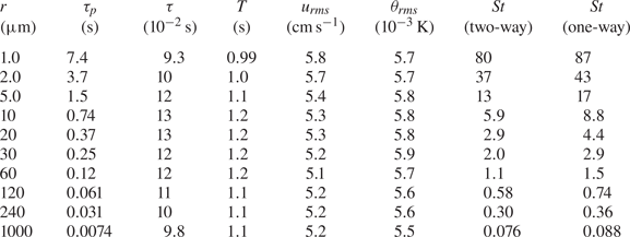
Figure 6 shows the snapshots of particle distribution for the two-way momentum coupling case. Due to momentum coupling, inertial clustering of particles is clearly observed for  $St=1.1$ (figure 6b, $r=60\,\mathrm {\mu }$m). Similar particle distributions were obtained for the one-way momentum coupling case.

Figure 6. Particle distribution obtained by a simulation with two-way momentum coupling. Particle radius is 1000, 60 and 5  $\mathrm {\mu }$m from (a) to (c), respectively. Only particles within a slice $-\Delta x/2 < z < -\Delta x/2$ are shown.
Figure 7(a) shows the ratio  $\langle \theta ^{2}\rangle _V/\theta _0^{2}$ at the statistically steady state. Note that, for cases with momentum coupling, the average over particles ( $\langle \, \rangle _p$) is generally different from that over fluid volume ( $\langle \, \rangle _V$). Since our focus is on modulation of fluid temperature fluctuations, we use the average over fluid volume. The results for the one-way momentum coupling case (red triangles) are very similar to those for the case without momentum inertia (blue squares). On the other hand, the results for the two-way momentum coupling case (black dots) show significantly greater values than the other two cases. Several black dots are even greater than unity, indicating that the fluid temperature variance is increased by particles for these runs.

Figure 7. (a) Same as figure 3(c) but for one- and two-way momentum coupling cases (red triangles and black dots, respectively) with  $N_{grid}=128$ and $\phi _{\theta }=0.1$. Note also that the vertical axis is $\langle \theta ^{2}\rangle _V/\theta _0^{2}$ instead of $\langle \theta ^{2}\rangle _p/\theta _0^{2}$. Blue squares are the same as in figure 3(c) where the momentum inertia of the particle is neglected. (b) Same as (a) for the two-way momentum coupling case except that the vertical axis is $\langle \theta ^{2}\rangle _V/\theta _c^{2}$, where $\theta _c^{2}$ is defined by (E7). See discussion in the main text.
The increase in the fluid temperature variance for the two-way momentum coupling case is caused by attenuation of turbulent kinetic energy by particles. In scalar turbulence, the cascade of scalar variance to smaller scales is mainly driven by the large-scale eddies, and its time scale is roughly estimated by the large-eddy turnover time  $T$. Since the injection rate is kept at a constant $\chi _0$ in the present study, the fluid temperature variance without particles, $\theta _0^{2}$, is determined by the scaling relationship (3.16). On the other hand, when the turbulent kinetic energy is attenuated by particles due to two-way momentum coupling, the time scale of the cascade becomes longer, which leads to an increase in the fluid temperature variance. This increase can be estimated by the following scaling argument. If modulation of the fluid temperature variance is solely caused by the change in the large-eddy turnover time (and not by two-way thermal coupling), the variance is expected to become $\theta _c^{2}$ which is determined by
 \begin{equation} \chi_0 \sim \frac{\alpha}{T_1} \theta_c^{2}, \end{equation}
where  $T_1$ and $T$ are the large-eddy turnover time of turbulence with and without the effect of two-way momentum coupling, respectively ( $T_1>T$). By equating (E6) with (3.16), we obtain the relationship between $\theta _c^{2}$ and $\theta _0^{2}$ as follows:
 \begin{equation} \theta_c^{2} = \left( \frac{T_1}{T} \right)\theta_0^{2}, \end{equation}
which indicates  $\theta _c^{2} > \theta _0^{2}$ since $T_1>T$. This nominal value $\theta _c^{2}$ can be used to estimate the relative effect of turbulence attenuation on modulation of the fluid temperature variance.
Figure 7(b) shows the same as figure 7(a) for the two-way momentum coupling case, except that the vertical axis is replaced by the ratio  $\langle \theta ^{2}\rangle _V/\theta _c^{2}$. By using $\theta _c^{2}$ instead of $\theta _0^{2}$, we removed the contribution of the increase in the large-eddy turnover time to modulation of the fluid temperature variance. All results in figure 7(b) are now smaller than unity and agree well with the theoretical curve (grey dashed curve), as for the one-way momentum coupling case and the case without momentum inertia in figure 7(a) (red triangles and blue squares). These results indicate that the increase in the variance for the two-way momentum coupling case shown in figure 7(a) (black dots) is mostly caused by the attenuation of turbulent kinetic energy by particles which in turn leads to the increase in the large-eddy turnover time, and also that inertial clustering and associated phenomena are not so important in the modulation of the fluid temperature variance. In addition, these results also confirm that the theoretical prediction (3.19) (grey dashed curves in figure 7) is still useful for the study of cases with momentum coupling.


 Open access