


1. Introduction
Invariant solutions of the Navier–Stokes equations play a key role for the dynamics of transitional shear flows (Kawahara, Uhlmann & van Veen Reference Kawahara, Uhlmann and van Veen2012). These solutions, in the form of equilibria, travelling waves and periodic orbits, have been computed for many canonical shear flows including pipe flow (Faisst & Eckhardt Reference Faisst and Eckhardt2003), plane Couette flow (Gibson, Halcrow & Cvitanović Reference Gibson, Halcrow and Cvitanović2009), plane Poiseuille flow (Waleffe Reference Waleffe2003) and asymptotic suction boundary layer flow (Kreilos et al. Reference Kreilos, Veble, Schneider and Eckhardt2013). Invariant solutions are mostly found in small periodic domains, or ‘minimal flow units’ (Jiménez & Moin Reference Jiménez and Moin1991). Later investigations have considered extended domains and identified localised invariant solutions that capture large scale flow patterns like turbulent spots, stripes and puffs (Avila et al. Reference Avila, Mellibovsky, Roland and Hof2013; Brand & Gibson Reference Brand and Gibson2014; Reetz, Kreilos & Schneider Reference Reetz, Kreilos and Schneider2019; Reetz & Schneider Reference Reetz and Schneider2020).
The first family of spatially localised invariant solutions in shear flows were calculated by Schneider, Marinc & Eckhardt (Reference Schneider, Marinc and Eckhardt2010b) in plane Couette flow. This includes equilibria and travelling waves, which are equilibria in a frame of reference moving relative to the laboratory frame. These localised invariant solutions in plane Couette flow are specifically noteworthy because they exhibit the characteristic behaviour of homoclinic snaking (see the review by Knobloch Reference Knobloch2015) under parametric continuation (Schneider, Gibson & Burke Reference Schneider, Gibson and Burke2010a). Homoclinic snaking is a process previously observed in many dissipative pattern-forming systems such as binary-fluid convection systems (Batiste et al. Reference Batiste, Knobloch, Alonso and Mercader2006) and optical systems (Firth, Columbo & Maggipinto Reference Firth, Columbo and Maggipinto2007), by which localised solutions grow in one direction while undergoing a sequence of successive saddle-node bifurcations (Woods & Champneys Reference Woods and Champneys1999). Homoclinic snaking manifests itself by a characteristic snakes-and-ladders structure in the bifurcation diagram (Burke & Knobloch Reference Burke and Knobloch2007).
A well-studied one-dimensional model system which supports localised solutions that exhibit homoclinic snaking is the Swift–Hohenberg equation  $\partial _t u=r u + (1+\partial ^2_x)^2 u+\mathcal {N}(u)$, for a real-valued function $u(x)$ on the real axis with $r$ the bifurcation parameter and a nonlinearity $\mathcal {N}(u)$ (Burke & Knobloch Reference Burke and Knobloch2006, Reference Burke and Knobloch2007; Beck et al. Reference Beck, Knobloch, Lloyd, Sandstede and Wagenknecht2009; Knobloch, Uecker & Wetzel Reference Knobloch, Uecker and Wetzel2019). Several variants of the Swift–Hohenberg equation with differing forms of the nonlinear term have been considered. Most studied are both a quadratic-cubic $\mathcal {N}=b_2 u^2 - u^3$ and a cubic-quintic $\mathcal {N} = b_3 u^3 - u^5$ nonlinearity, where $b_2$ and $b_3$ are adjustable parameters. For both nonlinear terms, the Swift–Hohenberg equation supports localised solutions arranged in a snakes-and-ladders bifurcation structure. The localised invariant solutions of the Navier–Stokes equations in plane Couette geometry share remarkably similar properties with solutions of the Swift–Hohenberg equation with the cubic-quintic nonlinearity (Schneider et al. Reference Schneider, Gibson and Burke2010a):
(i) First, the bifurcation diagram with its characteristic snakes-and-ladders structure is almost indistinguishable from that of the Swift–Hohenberg equation.
(ii) Second, the three-dimensional snaking solutions of the Navier–Stokes equations very closely resemble one-dimensional snaking solutions of Swift–Hohenberg, when three-dimensional velocity fields are averaged in the downstream direction and zero sets of downstream velocity are visualised as a function of the spanwise coordinate.
The almost perfect resemblance of three-dimensional Navier–Stokes and one-dimensional Swift–Hohenberg solutions is observed for the downstream wavelength of  $4 {\rm \pi}$ studied in Schneider et al. (Reference Schneider, Gibson and Burke2010a). Subtle modifications related to internal deformations of the three-dimensional velocity field appear when the downstream wavelength changes, but the characteristic snakes-and-ladders structure remains intact (Gibson & Schneider Reference Gibson and Schneider2016). Why localised solutions of the three-dimensional Navier–Stokes equations closely resemble solutions of the one-dimensional Swift–Hohenberg equation and are organised in a snakes-and-ladders bifurcation structure is not fully understood. Homoclinic snaking in model systems including the Swift–Hohenberg equation is studied in detail by approaches including spatial dynamics, where the fixed-point equation is treated as a dynamical system in the spatial coordinate that indicates the direction in which solutions are localised (Champneys Reference Champneys1998; Knobloch Reference Knobloch2015). A localised snaking solution corresponds to a homoclinic orbit in space that starts from the homogeneous background state, approaches a periodic orbit representing the internal pattern of the localised solution and returns to the homogeneous background. Discrete symmetries of the specific equation control whether such homoclinic orbits in space generically exist and whether an equation supports homoclinic snaking (Burke, Houghton & Knobloch Reference Burke, Houghton and Knobloch2009). In both the Navier–Stokes solutions and in solutions of the Swift–Hohenberg equation with cubic-quintic nonlinearity, the snakes-and-ladders bifurcation structure is composed of two pairs of intertwined snaking branches along which the solutions are invariant under discrete symmetries that are part of the equivariance group of the respective system. The snaking branches of symmetric solutions are connected by so-called rungs, which emerge in symmetry-breaking pitchfork bifurcations. The rungs do not possess discrete symmetries and, together with the snaking branches, form the snakes-and-ladders structure, as schematically shown in figure 1.

Figure 1. Schematics of the snakes-and-ladders bifurcation structure observed in both the one-dimensional Swift–Hohenberg equation with cubic-quintic nonlinearity and the three-dimensional Navier–Stokes equations in the plane Couette geometry. Two pairs of intertwined snaking branches of localised solutions undergo sequences of saddle-node bifurcations under continuation in a control parameter of the respective system. Each snaking curve represent two symmetry-related branches of solutions with equal norm. All solutions along the snaking branches are invariant under discrete symmetries. The symmetric snaking branches are connected by asymmetric rung state branches.
The equivariance group of the Swift–Hohenberg equation with cubic-quintic nonlinearity includes the even symmetry  $R_1 : x\rightarrow -x, u\rightarrow u$ and the odd symmetry $R_2 : x\rightarrow -x, u\rightarrow -u$. To investigate the importance of discrete symmetries for the snaking structure of the Swift–Hohenberg equation with cubic-quintic nonlinearity, Houghton & Knobloch (Reference Houghton and Knobloch2011) introduced an additional quadratic term in the equation to break the odd symmetry of the system $R_2$. When the amplitude $\epsilon$ of this symmetry-breaking term $\epsilon u^2$ is increased from zero, the bifurcation structure changes. One pair of snaking branches breaks into disconnected pieces while the other pair splits into two distinct curves in an amplitude versus $r$ bifurcation diagram. Those curves are connected by z- and s-shaped non-symmetric solution branches that are composed of solutions that for $\epsilon =0$ form rungs and the snaking branches that disappear when the symmetry is broken.
In the Swift–Hohenberg equation with cubic-quintic nonlinearity, breaking a specific discrete symmetry destroys the snakes-and-ladders bifurcation structure that solutions of Navier–Stokes in the plane Couette geometry remarkably well resemble. Discrete symmetries are transformations of one-dimensional functions in the context of the Swift–Hohenberg equation, while for Navier–Stokes, they represent transformations of three-dimensional velocity fields. Consequently, there is no obvious correspondence between specific symmetry transformations in both systems and the effect of breaking a specific symmetry in Swift–Hohenberg cannot be directly translated to Navier–Stokes. To investigate the significance of discrete symmetries of the three-dimensional Navier–Stokes equations, we therefore break a symmetry of plane Couette and study the structural stability of the snakes-and-ladders structure under controlled symmetry breaking. We specifically apply wall-normal suction to break the rotational symmetry of plane Couette flow. At small amplitude, suction modifies the snakes-and-ladders structure of plane Couette flow in the same way a quadratic term modifies the snakes-and-ladders structure of the Swift–Hohenberg equation with the cubic-quintic nonlinearity. At higher values of suction velocity, the snaking branches that remain intact at small suction velocity also break down. The solutions form separated branches which involve solutions that can be followed to zero suction velocity but are not part of the snakes-and-ladders structure of plane Couette flow without suction. We thereby identify previously unknown localised solutions of plane Couette flow that exist in a much wider range of Reynolds numbers than the snaking solutions of equal downstream wavelength studied previously. The structural modifications of the bifurcation structure at large amplitude of the symmetry-breaking terms is not observed in the Swift–Hohenberg system, where increasing the amplitude of the quadratic term transforms the snakes-and-ladders structure into a modified snakes-and-ladders structure similar to the bifurcation structure of the localised solutions of the Swift–Hohenberg equation with quadratic-cubic nonlinearity. Thus, at small suction amplitudes, suction has a similar effect as the symmetry-breaking term within the cubic-quintic Swift–Hohenberg case, while at larger suction amplitudes, the bifurcation structure of three-dimensional Navier–Stokes solutions significantly differs from that of the analogous Swift–Hohenberg problem. Both in the one-dimensional model system and in the full three-dimensional Navier–Stokes problem, the initial breakdown of the snakes-and-ladders structure can be explained in terms of symmetry breaking.
This manuscript is organised as follows: in § 2, we introduce the plane Couette system with wall-normal suction and discuss its symmetry properties. Section 3 reviews the snaking solutions and the snakes-and-ladders structure of plane Couette flow at zero suction. Section 4 presents the key observations on how wall-normal suction modifies the snaking structure. In § 5, features of the modified snaking structure are discussed and related to symmetry properties, including symmetry subspaces of the flow. Section 6 discusses the breakdown of the snakes-and-ladders structure for large values of suction and reveals the existence of new branches of localised solutions of plane Couette flow without suction. In the final § 7, results are summarised and an outlook for future work is provided.
2. System and methodology
Plane Couette flow (PCF) is the flow of a Newtonian fluid between two parallel plates at a distance of  $2H$ which move in opposite directions with a constant relative velocity of $2U_w$. The laminar solution of the Navier–Stokes equations in PCF is a linear profile. We investigate the effect of wall-normal suction (see figure 2) on the snaking solutions of PCF. The wall-normal suction modifies the laminar flow. After non-dimensionalisation of the velocities with respect to half of the relative velocity of the plates, $U_w$, and the lengths with respect to half of the gap width between the plates, $H$, the laminar solution takes the form
 \begin{equation} \boldsymbol{U}(y)=U_x(y)\hat{\boldsymbol{e}}_x-V_s\hat{\boldsymbol{e}}_y, \end{equation}
where the coordinate system  $(x, y, z)$ is aligned with the streamwise $(\hat {\boldsymbol {e}}_x)$, the wall-normal $(\hat {\boldsymbol {e}}_y)$ and the spanwise directions $(\hat {\boldsymbol {e}}_z)$; $\boldsymbol {U}(y)$ is the laminar solution; $V_s$ is the non-dimensionalised wall-normal suction velocity; and
 \begin{equation} U_x(y)=1-\frac{1}{\sinh(-Re V_s)}(\exp(-Re V_s)-\exp(-y Re V_s)). \end{equation}
Decomposition of the total velocity into the laminar solution,  $\boldsymbol {U}(y)$ as a base flow, and the deviation from the laminar solution, $\boldsymbol {u}(x,y,z,t)$, yields the Navier–Stokes equations in perturbative form
 \begin{equation} \frac{\partial \boldsymbol{u}}{\partial t} + U_x(y)\frac{\partial \boldsymbol{u}}{\partial x}-V_s\frac{\partial \boldsymbol{u}}{\partial y}+v\frac{\textrm{d} U_x(y)}{\textrm{d} y}\hat{\boldsymbol{e}}_x+\boldsymbol{u}\boldsymbol{\cdot}\boldsymbol{\nabla}\boldsymbol{u}=-\boldsymbol{\nabla} p + \frac{1}{Re}\nabla^2\boldsymbol{u}, \end{equation}
where the Reynolds number is defined as  $Re=UH/\nu$, with $\nu$ the kinematic viscosity of the fluid. The boundary conditions for $\boldsymbol {u}$ are periodic in the streamwise and the spanwise directions,
 \begin{equation} \left.\begin{array}{c@{}} \boldsymbol{u}(-L_x/2,y,z,t) = \boldsymbol{u}(L_x/2,y,z,t),\\ \boldsymbol{u}(x,y,-L_z/2,t) = \boldsymbol{u}(x,y,L_z/2,t), \end{array}\right\} \end{equation}
where  $L_x$ and $L_z$ are the length and width of the computational domain in the streamwise and the spanwise directions, respectively. At the top and bottom plate Dirichlet conditions
 \begin{equation} \left.\begin{array}{c@{}} \boldsymbol{u}(x,1,z,t) = (1,-V_s,0),\\ \boldsymbol{u}(x,-1,z,t) = (-1,-V_s,0), \end{array}\right\} \end{equation}
are satisfied. A zero pressure gradient in both the streamwise and spanwise directions is imposed.

Figure 2. Schematic of plane Couette flow with wall-normal suction. Lengths and velocities are non-dimensionalised with respect to half the distance between the two planes  $H$ and half the relative velocity of the planes $U_w$, respectively. The Reynolds number $Re=U_w H/\nu$, with $\nu$ the kinematic viscosity of the fluid, and the non-dimensionalised suction velocity $V_s$ constitute the two control parameters of the system.
Following Gibson & Schneider (Reference Gibson and Schneider2016), we present bifurcation diagrams in terms of energy dissipation of the deviation from the laminar solution, normalised by the length of the channel  $L_x$. The considered solutions are localised and thus independent of the width $L_z$ of the domain. Consequently, we do not normalise by the width $L_z$. The streamwise averaged energy dissipation for an equilibrium or travelling wave solution equals the energy input rate $I$ and can be expressed as
 \begin{equation} D=I=\frac{1}{2L_x}\int_{-L_z/2}^{L_z/2}\int_{-L_x/2}^{L_x/2}\left(\left.\frac{\partial \boldsymbol{u}}{\partial y}\right|_{y=-1}+\left.\frac{\partial \boldsymbol{u}}{\partial y}\right|_{y=1}\right) {\textrm{d}\kern0.02em x}\, \textrm{d}z, \end{equation}
in units of  $U_w^2$. Here, $D$ serves as a measure for the width of a localised solution that approaches laminar flow ( $\boldsymbol {u}=0)$ and only generates non-zero dissipation in the non-laminar part of the solution.
PCF ( $V_s=0$) is equivariant under continuous translations in the $x$ and $z$ directions, discrete reflection in the $z$ direction and a discrete rotation of $180\,^\circ$ around the $z$ axis. The rotation is equivalent to two successive discrete reflections in the $x$ and $y$ directions. Following the conventions of Gibson, Halcrow & Cvitanović (Reference Gibson, Halcrow and Cvitanović2008), these symmetry transformations, under which the governing equations and the boundary conditions of PCF are equivariant, are expressed as
 \begin{equation} \left.\begin{array}{c@{}} \sigma_z : [u,v,w](x,y,z) \rightarrow[u,v,-w](x,y,-z),\\ \sigma_{xy} : [u,v,w](x,y,z) \rightarrow[-u,-v,w](-x,-y,z),\\ \tau(\delta x, \delta y) : [u,v,w](x,y,z) \rightarrow[u,v,w](x+\delta x,y,z+\delta z), \end{array}\right\} \end{equation}
where  $\delta x$ and $\delta z$ are arbitrary displacements in the streamwise and the spanwise directions, respectively. All products of the reflection symmetry, $\sigma_z$, the rotational symmetry, $\sigma_{xy}$, and the translational symmetry, $\tau$, compose the symmetry, or equivariance, group of PCF ( $V_s=0$). The equivariance group contains the discrete symmetries under which the snaking solutions are invariant. These are the inversion symmetry $\sigma _{xyz}$ for the snaking equilibria and the shift–reflect symmetry $\tau _x\sigma _z$ for the snaking travelling waves
 \begin{equation} \left.\begin{array}{c@{}} \sigma_{xyz} : [u,v,w](x,y,z) \rightarrow[-u,-v,-w](-x,-y,-z),\\ \tau_x\sigma_{z} : [u,v,w](x,y,z) \rightarrow[u,v,-w](x+L_x/2,y,-z), \end{array}\right\} \end{equation}
where  $\tau _x=\tau (L_x/2,0)$ is a half-box translation in the streamwise direction. A non-zero wall-normal suction velocity breaks the rotational symmetry of the system, $\sigma _{xy}$. Therefore, for PCF with a non-zero wall-normal suction, the equivariance group consists of all products of the translational symmetry, $\tau$, and the reflection symmetry, $\sigma _z$. Consequently, for non-zero wall-normal suction, the inversion symmetry $\sigma _{xyz}$ of PCF is broken; PCF with a non-zero wall-normal suction is not equivariant under the inversion symmetry.
The significance of symmetries for both the dynamics of a flow and for its bifurcation structure has been described in detail (Crawford & Knobloch Reference Crawford and Knobloch1991; Chossat & Lauterbach Reference Chossat and Lauterbach2000; Golubitsky & Stewart Reference Golubitsky and Stewart2002): first, all velocity fields which are invariant under the action of a symmetry contained in the equivariance group form a symmetry subspace within the system's state space. If an initial condition  $\boldsymbol {u}$ is located in a symmetry subspace, its evolution under the governing equations remains in the same symmetry subspace. Second, if an equilibrium or travelling wave solution is invariant under a symmetry and thus located in a symmetry subspace, parametric continuation will not change the symmetry of the solution; instead, the entire continuation branch remains in the same symmetry subspace. Symmetries can only change if the branch is created or terminates in a symmetry-breaking bifurcation such as a pitchfork bifurcation. Third, the equivariance of the system under symmetry transformations implies that if an equilibrium or travelling wave solution is not invariant under a symmetry contained in the equivariance group of the system, then the action of that symmetry on the solution creates an additional solution. Two equilibria/travelling waves that are related by a symmetry have the same global integrated properties such as dissipation, and thus are represented by a single curve in bifurcation diagrams presenting the global integrated property as a function of a control parameter.
The invariant solutions presented in this study including equilibria and travelling waves are identified numerically using the Newton–Krylov–hookstep (Viswanath Reference Viswanath2007) root-finding tools contained in Channelflow 2.0 (www.channelflow.ch). To construct the required Krylov subspace, Channelflow employs successive time integrations of the Navier–Stokes equations to evaluate the action of the Jacobian by finite differencing. For integrating the Navier–Stokes equations in time, a third-order accurate semi-implicit backward differentiation scheme is used together with a pseudo-spectral Fourier–Chebyshev–Fourier discretisation. In the homogeneous streamwise and spanwise directions, we dealias the nonlinear term according to the 2/3 rule. The computational domain has a length of  $L_x = 4{\rm \pi}$, a width of $L_z=24{\rm \pi}$ and a height of $2H = 2$ and is discretised by $N_x=32$, $N_y=35$ and $N_z=432$ collocation points. All of the solutions are localised in the spanwise directions and are thus independent of the width of the computational domain.
3. Symmetry properties of snaking solutions in PCF without suction
The snaking solutions found by Schneider et al. (Reference Schneider, Gibson and Burke2010a) in PCF are shown in figure 3 together with their bifurcation diagram. The solutions are computed for a periodic box with length  $L_x=4{\rm \pi}$ and show the snakes-and-ladders structure characteristic of homoclinic snaking. Two snaking curves winding upward in dissipation while oscillating in Reynolds number represent equilibrium (EQ) and travelling wave (TW) solutions, respectively. Each of the curves, both for EQs and TWs represents two symmetry-related solution branches. Pairs of EQ solutions (labelled EQ1 and EQ2) and pairs of TWs (labelled TW1 and TW2) are related by the rotational symmetry of PCF, $EQ1 = \sigma _{xy}EQ2$, and $TW1 =\sigma _{xy}TW2$. The operation of the discrete rotational symmetry leaves global solution measures such as the norm or the streamwise averaged energy dissipation unchanged. Consequently, both symmetry-related branches appear as a single curve in the dissipation $D$ versus $Re$ bifurcation diagram. In the snaking region approximately in the range $169 < Re < 177$ the snaking solutions grow in the spanwise direction along the snaking curves while undergoing sequences of saddle-node bifurcations. At each saddle-node bifurcation an additional pair of streaks is added at the solution fronts, while the internal structure of the solutions remains unchanged (Schneider et al. Reference Schneider, Gibson and Burke2010a). As a result of the spatial growth, the dissipation of the snaking solutions increases along the snaking curves.

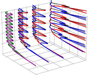
Figure 3. (a) A part of the snakes-and-ladders bifurcation structure of the localised invariant solutions in PCF in a box with a length of  $4{\rm \pi}$ and a width of $24{\rm \pi}$. The symmetry-related solutions are visualised at the points indicated on the bifurcation diagram: the velocity fields at point $(i)$ are two symmetry-related travelling waves; point $(ii)$ corresponds to two symmetry-related equilibrium solutions; and point $(iii)$ represents four symmetry-related rung states. All velocity fields are visualised in terms of the midplane streamwise velocity (red/blue contours) and the streamwise averaged cross-flow velocity (vector plots). In addition, the contour line of zero average streamwise velocity is presented. The red/blue streaks indicate $\pm 0.2 U_w$. The entire computational domain is shown. Note the localisation of all solutions in the spanwise direction.
The EQ solutions are invariant under the inversion symmetry,  $\sigma _{xyz}$ which is the product of the rotational symmetry, $\sigma _{xy}$, and the reflection symmetry, $\sigma _z$. A non-trivial invariant solution which is invariant under inversion is phase locked and can neither travel in the streamwise nor the spanwise direction so that the solution is an EQ and not a TW. In contrast, the TW solutions are invariant under a different symmetry, the shift–reflect symmetry, $\tau _x\sigma _z$ which locks only the $z$ phase of the solutions. As a result, the TWs are free to travel in the streamwise direction. Since the EQ solutions are invariant under the inversion symmetry ( $\boldsymbol {u}=\sigma _{xyz}\boldsymbol {u}$), the rotational symmetry relation between the two equilibria $EQ1=\sigma _{xy}EQ2$ reduces to $EQ1=\sigma _{xy}\sigma _{xyz}EQ2=\sigma _z 2$. Consequently, the rotational symmetry relation between the EQ solutions is equivalent to a mirror $z$-reflection symmetry relation between them. The two symmetry-related equilibria are thus mirror images with respect to the spanwise direction. For the TWs, their rotational symmetry relation implies that $TW1$ and $TW2$ travel in opposite directions but at equal phase speed.
In addition to the snaking branches, there are non-symmetric localised solutions which form rungs connecting the EQ branches to the TW branches. Rungs are created in pitchfork bifurcations close to the saddle-node bifurcations along the snaking branches. There are four rung solution branches corresponding to each curve in the bifurcation diagram (labelled R1, R2, R3 and R4). They each connect one of the two EQ branches to one of the two TW branches. Every pitchfork bifurcation on a specific EQ branch creates two rung states which each connect this specific EQ branch to one of the two TWs. Since the rung states are non-symmetric invariant solutions which are created in symmetry-breaking pitchfork bifurcations off symmetric invariant solutions, the two simultaneously created rungs are related to each other by the symmetry of the symmetric solution branch which is broken. This is either the inversion symmetry of the equilibria  $R1=\sigma _{xyz}R2$ and $R3=\sigma _{xyz}R4$ or the shift–reflect symmetry of the TWs. The shift–reflect symmetry relation between the two rung state solutions connecting to one TW can be interpreted as only a $z$-reflection symmetry relation $\sigma _z$ between the rungs $R1 = \sigma _z R3$ and $R2 = \sigma _z R4$, because the shift is absorbed in the continuous translation symmetry for a solution that is not phase locked but free to travel in the streamwise direction. Hence, at any Reynolds number, the four rung state solutions have the same dissipation, and the four branches of the rung states in the bifurcation diagram are represented by a single curve. The symmetry relations between all branches of the snakes-and-ladders structure in PCF are schematically summarised in figure 4 together with all relevant invariant symmetry subspaces. The two equilibria are located in the inversion symmetry subspace and they are related to each other by a $z$-reflection symmetry. The two TWs are in the subspace of the shift–reflect symmetry, and are related by the rotational symmetry, $\sigma _{xy}$. The rung state solutions are non-symmetric and live outside these two symmetry subspaces.

Figure 4. Symmetry relations (arrows) between solution branches of PCF without suction. The pair of travelling waves  $TW1/TW2$ is located within an invariant symmetry subspace (shaded orange ellipse). Likewise, the pair of equilibria $EQ1/EQ2$ shares a symmetry subspace (shaded cyan ellipse). All rungs $R1$,
$R1$,  $R2$,
$R2$,  $R3$ and $R4$ are non-symmetric.
4. Modified snakes-and-ladders bifurcation structure for non-vanishing suction
Wall-normal suction breaks the inversion symmetry of PCF and leads to modifications of all discussed solution branches. As a result of the broken rotational symmetry, any symmetry subspace or symmetry relation originating from rotational symmetry is not present for non-zero suction velocity. Consequently, for non-zero suction, there is no inversion symmetry subspace,  $\sigma _{xyz}$ and states that are inversion-symmetric equilibria at zero suction should travel in the streamwise and the spanwise directions. Moreover, the rotational symmetry relation between the two TW branches and the inversion symmetry relation between rung states vanishes. Figure 5(a) schematically indicates the configuration of symmetry subspaces and symmetry relations of states in the presence of wall-normal suction. These modified symmetry relations caused by non-vanishing suction are expected to impact both the bifurcation structure and the solutions themselves. In the following, we first discuss modifications of the bifurcation diagram due to suction. Then, we present how solutions along the solution branches are modified.

Figure 5. (a) Symmetry relations (arrows) between solution branches of PCF in the presence of non-vanishing wall-normal suction velocity. For  $V_s\neq 0$, the inversion symmetry relation $\sigma _{xyz}$ between $R1$ and $R2$ and between $R3$ and $R4$, the rotational symmetry relation $\sigma _{xy}$ between $TW1$ and $TW2$ and the inversion symmetry subspace, all present for $V_s=0$ (see figure 4) are broken. As a result of the broken inversion symmetry of the equilibria in the presence of suction, these solutions travel in both streamwise and spanwise directions and do not remain EQ solutions. The $EQ1$ and $EQ2$ labels in (a) are carried over from PCF without suction and indicate remnants of EQ solutions. (b) For finite values of suction, these remnants of equilibria together with remnants of the rung states form pairs of symmetry-related returning state, RS/RS′, and connecting state, CS/CS′, branches. These are discussed in § 4.1.
4.1. Effect of suction on the bifurcation diagram
Figure 6 shows how the snakes-and-ladders bifurcation structure is modified when wall-normal suction is applied. The two TW branches undergoing snaking are symmetry related at zero suction and thus appear as a single curve. For non-zero suction, the symmetry relating both branches is not contained in the equivariance group. Consequently, the symmetry relation vanishes and the two TW branches split.

Figure 6. Modification of the snaking diagram with increasing wall-normal suction. The suction velocity is increased from  $V_s = 0$ (a) to $V_s=10^{-4}$ (b) and $V_s=2\times 10^{-4}$ (c). (a) TW (magenta) and EQ (green) snaking branches are shown together with rungs (black). (b,c) The TW branch splits into $TW1$ (thick red) and $TW2$ (thick blue). The snaking EQ branch has broken into disconnected segments and together with remnants of rungs forms returning states, RS, and connecting states, CS. Two types of RS (thin red/blue) connect to $TW1$/ $TW2$, respectively. The CS states (thin black) connect $TW1$ and $TW2$.
Solutions cannot only be followed from zero to positive suction velocity  $V_s=+|V_s|$ but also to negative values $V_s=-|V_s|$. The latter physically imply blowing through the wall. Since the rotational symmetry $\sigma _{xy}$, relating $TW1$ to $TW2$ at $V_s=0$ and broken by suction, transforms a flow with suction to a flow with equal amplitude blowing, the TW branches for inverted suction velocity are related by
 \begin{equation} TW2 |_{V_s}=\sigma_{xy} TW1 |_{-V_s}. \end{equation}
For non-zero suction, there is therefore only a symmetry relation between the two TWs if the direction of suction is inverted. For a fixed positive value of  $V_s$ the two TW branches are, however, not symmetry related, causing the observed split of both TW branches. The two TW branches remain continuous and undergo snaking, but the critical $Re$ at which saddle-node bifurcations occur alternates. Following the terminology of Knobloch (Reference Knobloch2015), we refer to the piece of a snaking curve between two forward saddle-node bifurcations including a backward saddle-node bifurcation as an oscillation in the snaking branch. In the snaking region, both TW branches are composed of two alternating oscillations with different spans in Reynolds number, a narrow oscillation and a wide oscillation. Where TW branch $TW1$ undergoes a narrow oscillation the other one $TW2$ undergoes a wide oscillation. For the next pair of oscillations the situation reverses with, $TW1$ undergoing a wide, and $TW2$ a narrow oscillation.
EQ branches that undergo snaking in the zero suction case are invariant under the inversion symmetry, which is broken by suction. As a result, for non-zero suction, states that are inversion-symmetric equilibria at zero suction travel in the streamwise and the spanwise directions. The snaking EQ solution branches vanish. Instead the branch breaks into disconnected segments. The pitchfork bifurcations that – for the zero suction case – create rung states bifurcating from the EQ branches are broken by the wall-normal suction. In figure 7( $a$) a part of the bifurcation diagram enlarging one oscillation of the TWs for non-zero suction is shown. At non-zero suction the disconnected remnants of the EQ branches together with remnants of rung states form new branches that connect to TW branches (see figure 5). These branches fall into two groups. Some branches emerge in a pitchfork bifurcation on one of the TW branches (point $(10a)$ in figure 7 $a$) and terminate on the same TW branch in another pitchfork bifurcation (point $(10g)$ in figure 7 $a$). Hereafter, these branches are called returning states, RS, shown separately in figure 7( $c$). There are two RS branches, which are related by a $z$-reflection symmetry, RS′ $= \sigma _z$ RS. All other non-symmetric branches connect $TW1$ to $TW2$ (from point $(10b)$ to point $(10h)$ in figure 7 $a$). These branches are, hereafter, referred to as connecting states, CS, shown separately in figure 7( $d$). In the continuation diagram, each CS curve represents two symmetry-related branches, CS′ $= \sigma _z$CS, which bifurcate from the TW branches in pitchfork bifurcations.

Figure 7.  $(a)$ One oscillation of the two TWs at $V_s=10^{-4}$. The velocity fields at the indicated points are visualised in figures 8 and 10. The colour coding is the same as in figure 6. $(b)$ Variation of the spanwise wave speed illustrating the two symmetry-related RS (solid and dashed blue) and CS (solid and dashed black) branches. (c,d) Separately show the RS ( $c$) and CS ( $d$) branches at $V_s=10^{-4}$. The snaking equilibria (dashed green), the snaking TWs (dashed magenta) and rung states (dashed black) at $V_s=0$ are included for reference. The RS and CS branches for non-zero suction are formed by remnants of the rungs and the snaking EQ solution branches of the system without suction.
The RS branches as well as the CS branches form closed bifurcation loops, as every branch has a symmetry-related counterpart starting and terminating in the same pitchfork bifurcation on TW branches. The loops can be directly observed in figure 7( $b$) where solutions are shown in terms of dissipation versus spanwise wave speed. The spanwise wave speed differentiates between both $z$-reflection symmetry-related branches. The spanwise wave speed of the two symmetry-related branches has the same magnitude but opposite sign. Due to their shift–reflect symmetry, the spanwise wave speed of the TW branches is zero.
4.2. Evolution of the velocity fields on the solution branches
Each saddle-node bifurcation along the snaking branches is associated with spanwise growth of the solution, as evidenced by the increasing value of dissipation. The neutral eigenmode associated with each saddle-node bifurcation is localised at the fronts of the localised solution where the spatially periodic internal pattern connects to unpatterned laminar flow (Schneider et al. Reference Schneider, Gibson and Burke2010a). When the snaking branch undergoes a saddle-node bifurcation, additional structures in the form of downstream streaks together with associated pairs of counter-rotating downstream vortices are added to the solution. The solution thereby grows while its interior structure remains essentially unchanged.
Both TW snaking branches  $TW1$ and $TW2$ are invariant under shift–reflect symmetry. This symmetry is preserved and not broken by the saddle-node bifurcations along the branch. Consequently, the saddle-node bifurcations simultaneously add structures symmetrically at both fronts of the TW. Figure 8 shows the evolution of the TWs in the snaking region for one oscillation. In this range, $TW1$ undergoes a wide oscillation and $TW2$ a narrow oscillation. Although the symmetry relation between $TW1$ and $TW2$ is broken for non-zero suction, for small values of the suction velocity the velocity fields visually still appear as if they were related by rotational symmetry, as shown in figure 9.


Figure 9. Comparison between  $TW1$ (red), $TW2$ (blue) and $\sigma _{xy} TW2$ (dashed blue) for $V_s=10^{-4}$. The contour line of zero average streamwise velocity is shown for the same states as in figure 8 ( ${c,\kern-0.06em d}$). At the considered small suction, the two TWs remain approximately symmetry related although the symmetry $\sigma _{xy}$ has been broken.
Figure 10 visualises the velocity fields of the RS and the CS branches at the points indicated in figure 7( $a$). Each point along both branches corresponds to two velocity fields related by $z$-reflection symmetry $\sigma _z$. We only visualise one of the two symmetry-related velocity fields. Neither the RS nor the CS solutions are invariant under any discrete symmetry. Consequently, the growing and shrinking of the solution along the branch is not symmetric. To visualise changes in the velocity field along the branch, we overlay two successive solutions shown in figure 10. Figure 11 shows the zero contour line of the average streamwise velocity of two consecutive velocity fields. The differences are small and located at the fronts. To further highlight the small differences and reveal growing and shrinking of the solution, contours of the amplitude difference of the average streamwise velocity $|\langle u_2 \rangle _x| - |\langle u_1 \rangle _x|$ are visualised.


Figure 11. The variations of velocity field along the RS branch (a,c,e) and the CS branch (b,d,f): overlay of zero contour lines of average streamwise velocity for pairs of velocity fields shown in figure 10 as dashed blue/solid red lines. (10a)/(10c) (a), (10c)/(10e) (c), (10e)/(10g) (e); (10b)/(10d) (b), (10d)/(10f) (d), (10f)/(10h) (f). Differences are visible close to the fronts. Colours indicate contours of the amplitude difference of the average streamwise velocity  $|\langle u_2 \rangle _x| - |\langle u_1 \rangle _x|$ with yellow/cyan corresponding to $\pm 0.13 U_w$. Along the RS branch (a,c,e), the envelope of the localised solutions shifts to the left, grows symmetrically and shifts to the right. After the sequence, the contour line remains centred at a maximum. Along the CS branch the structure shifts left, grows symmetrically and shifts left again. As a result, the contour line in the centre of the periodic pattern turns from a maximum into a minimum.
The RS branch (thin blue line in figure 7) bifurcates in a pitchfork bifurcation from  $TW2$ at $(10a)$. Towards $(10c)$, while decreasing in $Re$, the solution increases in strength at its left front and weakens on its right. One may describe the localised solutions as a superposition of a periodic pattern with an envelope that supports the internal core structure and damps the exterior towards laminar flow. The change of the solution along $(10a) \to (10c)$ corresponds to a left shift of the envelope (see figure 11a). From $(10c) \to (10e)$, close to the next saddle-node bifurcation, the velocity field gets stronger at both sides (see figure 11c). This segment of the RS branch is the remnant of an EQ branch at zero suction. The simultaneous and almost symmetric growth of the solution at both fronts along this segment resembles the growth of the EQ solution along the EQ branch at zero suction. Finally, from $(10e) \to (10g)$, close to the pitchfork bifurcation off $TW2$, the solution increases in strength on the right and weakens on the left front (figure 11e). The evolution along this part of the RS branch corresponds to a right shift of the envelope. Along a full RS branch, the envelope of the localised solutions first shifts to the left, then grows symmetrically and finally shifts to the right. After this sequence, both fronts have grown equally so that the RS branch acquires the symmetry of $TW2$ it bifurcated from. The symmetry-related branch RS′ $= \sigma _z$ RS bifurcates and reconnects to $TW2$ together with RS but the growth along the branch is inverted: a right shift is followed by symmetric growth and a final left shift.
The CS branch bifurcates from  $TW2$ in a pitchfork bifurcation at point $(10b)$. From $(10b) \to (10d)$ the velocity fields on the CS branch strengthens on the left and weakens on the right front, which corresponds to a left shift of the envelope (figure 11b). From $(10d) \to (10f)$ the velocity fields grow almost symmetrically at both fronts (figure 11d). This part of the CS branch is the remnant of an EQ branch at zero suction. Finally, from $(10f) \to (10h)$ the velocity fields again strengthen on the left front and weaken at the right front, corresponding to a left shift (figure 11f). At point $(10h)$ the CS branch connects to the $TW1$ branch in a pitchfork bifurcation. Along the CS branch the envelope first moves to the left, then grows symmetrically and finally moves to the left again. As a result of this growth sequence involving a net shift to the left, the centrally located low-speed streak (a blue streak in figure 10) is replaced by the neighbouring high-speed streak at the left (a red streak in figure 10), which now sits at the centre of the localised solution. A centrally located high-speed streak is characteristic of $TW1$. Consequently, the CS branch starts on $TW2$ and terminates on $TW1$. The symmetry-related branch CS′ $= \sigma _z$ CS bifurcates from $TW2$ and, as CS connects to $TW1$. However, along CS′ the solution exhibits a net shift to the right until the solution is no longer centred at a low-speed streak but on the next high-speed streak on the right. Since continuous shifts in the spanwise direction are part of the system's equivariance group, despite net shifts in opposite directions, both connecting state branches CS and CS′ connect to the same $TW1$ branch.
5. Relating properties of modified solutions to symmetry breaking
Non-vanishing suction velocity  $V_s$ causes splitting of the $TW1$ and $TW2$ branches and creates new CS and RS branches from the remnants of EQ and rung branches. In this section we relate these modifications of the snakes-and-ladders bifurcation structure due to the suction to the breaking of symmetries of PCF with zero suction.
5.1. Front growth controls bulk velocity and oscillation width
The mean pressure gradient in both spanwise and downstream directions is imposed to be zero and each solution selects its bulk velocity  $U_{bulk}$, the $y-z$ averaged streamwise velocity. Figure 12 shows the variation of the bulk velocity of the snaking solutions both for PCF with zero suction and for a suction velocity of $V_s=10^{-4}$. At zero suction, the EQ branch is invariant under $\sigma _{xyz}$, implying zero bulk velocity. The bulk velocity of the TW solutions periodically varies around zero as the solution undergoes snaking. The magnitude of the $U_{bulk}$ oscillations is independent of the spatial extent of the solution which suggests the non-zero bulk velocity is generated by the fronts, at which high- and low-speed streaks are growing symmetrically (Gibson & Schneider Reference Gibson and Schneider2016). While low-speed streaks are created, the bulk velocity becomes negative, and when high-speed streaks grow at the fronts the bulk velocity becomes positive. When suction is applied, the oscillations in bulk velocity are overlaid by an additional negative component that is linearly proportional in the dissipation. The linear dependence on dissipation and thereby size of the solution suggests that the linearly growing component of the bulk velocity is indicative of the internal structure of the solution remaining unchanged and creating a negative component proportional to the spatial extent of the solution. The oscillating component of the bulk velocity signal remains independent of the spatial extent and captures the growth process at the fronts.

Figure 12. Dissipation versus bulk velocity in the snaking region of plane Couette flow at zero suction (dashed) and for suction velocity  $V_s=10^{-4}$. Solution branches are indicated in the legend. At zero suction the bulk velocity of both TW branches oscillates around zero. With finite suction, an additional trend, linear in dissipation and thus size of the solution, is observed.
The front-mediated oscillations in bulk velocity relative to the linear trend are correlated with the width of snaking oscillations of the TW branches. Excursions to higher bulk velocity are observed when the branch undergoes a wide oscillation, i.e. a wider range of Reynolds numbers (see figure 7). Likewise, narrow oscillations are observed when the bulk velocity approaches local minima. Maxima of the bulk velocity are linked to high-speed streaks growing at the front while for minima in the bulk velocity, growing low-speed streaks are observed. Since  $TW1$ remains related to $TW2$ by the approximate though broken rotational symmetry $\sigma _{xy}$, a growth of high-speed streaks along the $TW1$ branch implies the growth of low-speed streaks along $TW2$ and vice versa. The growth of high- and low-speed streaks of approximately symmetry-related TW branches thus explains why wide and narrow oscillations of $TW1$ and $TW2$ both alternate and moreover occur such that a wide oscillation of $TW1$ coincides with a narrow one of $TW2$ and vice versa.
5.2. Splitting of the TWs
In PCF without suction, both TW solution branches,  $TW1$ and $TW2$, are represented by a single curve in the bifurcation diagram in terms of $D$ versus $Re$. Wall-normal suction breaks the rotational symmetry of the system $\sigma _{xy}$ and results in splitting of the TW solution branches (see figure 6). A subset of the bifurcation diagram is enlarged in figure 13( $a$), where dissipation $D$ as a function of $Re$ is presented for $TW1$ and $TW2$. The branches are shown for three values of the wall-normal suction velocity, $V_s=0$, $V_s=10^{-4}$ and $V_s=2\times 10^{-4}$. For non-zero suction, branches split so that $TW1$ and $TW2$ curves are symmetrically located around the zero suction curve, with equal distance but on opposing sides. The distance between both split curves grows linearly with the suction velocity. To rationalise this splitting behaviour we consider modifications of the solution of the governing equations at leading, namely linear, order in $V_s$. At zero wall-normal suction $V_s=0$, the laminar flow solution is a linear profile $\boldsymbol {U}(y)=y\hat {\boldsymbol {e}}_x$. Non-zero wall suction modifies the TW solutions $TW1$ and $TW2$. When decomposing the velocity into a laminar flow and deviations, this modification affects both the laminar base flow $\boldsymbol {U}$ and the deviation from the modified laminar base flow $\boldsymbol {u}$, as we will describe in this section.

Figure 13.  $(a)$ Bifurcation diagram of $TW1$ (red and magenta) and $TW2$ (blue and magenta) representing dissipation $D$ as a function of Reynolds number $Re$ for different values of the wall-normal suction velocity, $V_s=0$ (magenta line), $V_s=10^{-4}$ (dashed lines) and $V_s=2\times 10^{-4}$ (solid lines). For non-zero suction velocity, the branches of $TW1$ and $TW2$, which are represented by a single curve for $V_s=0$ (magenta), split symmetrically. They are located at the same distance but on opposite sides of the curve with $V_s=0$. $(b)$ Dissipation $D$ versus streamwise wave speed $c_x$ of $TW1$ (red) and $TW2$ (blue) for the same values of the wall-normal suction velocity as in $(a)$. The values of the suction velocity are indicated on the curves in the figure. The wave speeds of both $TW1$ and $TW2$ are shifted by equal amounts. The shift is proportional to the suction velocity $V_s$.
5.2.1. The modification of the laminar solution
At linear order in  $V_s$ the laminar solution reads
 \begin{equation} \boldsymbol{U} = \left(y+\frac{Re V_s}{2}(1-y^2)\right)\hat{\boldsymbol{e}}_x -V_s\hat{\boldsymbol{e}}_y. \end{equation}
Consequently, the modification of the laminar solution with respect to the laminar solution of PCF for zero suction velocity  $\boldsymbol {U}'=\boldsymbol {U}-\boldsymbol {U}_{V_s=0}$ is
 \begin{equation} \boldsymbol{U}' = V_s\left[\frac{Re}{2}(1-y^2)\hat{\boldsymbol{e}}_x -\hat{\boldsymbol{e}}_y\right] = V_s\boldsymbol{\bar{U}}(y,Re), \end{equation}
where  $\boldsymbol {\bar {U}}$ is a function of Reynolds number and the wall-normal coordinate $y$ only. Here, $\boldsymbol {\bar {U}}$ is independent of the suction velocity so that the laminar flow modification $\boldsymbol {U}'$ is linearly proportional to the suction velocity $V_s$.
5.2.2. The modification of the deviation from the laminar solution
The TW solutions  $TW1$ and $TW2$ are equilibria in a moving frame of reference that translate at their specific wave speeds $c_x$ in the $\hat {\boldsymbol {e}}_x$ direction with respect to the laboratory frame. The TW solutions thus satisfy the condition
 \begin{equation} (\boldsymbol{u}_t-c_x \hat{\boldsymbol{e}}_x)\boldsymbol{\cdot}\boldsymbol{\nabla} \boldsymbol{u}_t=-\boldsymbol{\nabla} p+\frac{1}{Re} \nabla^2 \boldsymbol{u}_t, \end{equation}
where  $c_x$ is the wave speed associated with the total velocity field $\boldsymbol {u}_t = \boldsymbol {U}(y)+\boldsymbol {u}(x,y,z)$. The solution of this equation $(\boldsymbol {u}_t, p,c_x)$ may be decomposed into three parts: the solution for zero suction, a modification of the laminar solution due to suction and the modification of the deviation from the laminar solution
 \begin{equation} \left.\begin{array}{c@{}} \boldsymbol{u}_t = \boldsymbol{u}_0 + \boldsymbol{U}' + \boldsymbol{u}'\\ p = p_0 + p'\\ c_x = c_{x0} + c'_x \end{array}\right\}, \end{equation}
where  $(\boldsymbol {u}_0, p_0,c_{x0})$ denotes the total solution for zero suction, $\boldsymbol {U}'$ is the modification of the laminar solution and $(\boldsymbol {u}', p',c'_x)$ is the modification of the deviation from the laminar solution. For small suction velocity, quadratic interactions among $\boldsymbol {U}'$, $\boldsymbol {u}'$ and $c'_x \hat {\boldsymbol {e}}_x$ resulting from the inertial term are neglected. At leading order, the condition for a TW solution at small suction thus reads
 \begin{align} &\boldsymbol{u}_0\boldsymbol{\cdot}\boldsymbol{\nabla} \boldsymbol{U}'+\boldsymbol{u}_0\boldsymbol{\cdot} \boldsymbol{\nabla} \boldsymbol{u}'+\boldsymbol{U}'\boldsymbol{\cdot} \boldsymbol{\nabla} \boldsymbol{u}_0+\boldsymbol{u}'\boldsymbol{\cdot} \boldsymbol{\nabla} \boldsymbol{u}_0-c_{x0}\boldsymbol{\cdot} \boldsymbol{\nabla} \boldsymbol{U}'-c_{x0}\boldsymbol{\cdot} \boldsymbol{\nabla} \boldsymbol{u}'-c'_x\boldsymbol{\cdot} \boldsymbol{\nabla} \boldsymbol{u}_0\nonumber\\ &\quad =-\boldsymbol{\nabla} p'+\frac{1}{Re}\nabla^2 \boldsymbol{U}'+\frac{1}{Re}\nabla^2 \boldsymbol{u}'. \end{align}
Rearranging using the base flow modifications at linear order in  $V_s$ (Equation 5.2), yields
 \begin{align} &V_s\left[\boldsymbol{u}_0\boldsymbol{\cdot} \boldsymbol{\nabla} \boldsymbol{\bar{U}}+\boldsymbol{\bar{U}}\boldsymbol{\cdot} \boldsymbol{\nabla} \boldsymbol{u}_0-c_{x0}\boldsymbol{\cdot} \boldsymbol{\nabla} \boldsymbol{\bar{U}}-\frac{1}{Re}\nabla^2 \boldsymbol{\bar{U}}\right] \nonumber\\ &\quad=-\boldsymbol{\nabla} p'+\frac{1}{Re}\nabla^2 \boldsymbol{u}'-\boldsymbol{u}_0\boldsymbol{\cdot} \boldsymbol{\nabla} \boldsymbol{u}'-\boldsymbol{u}'\boldsymbol{\cdot} \boldsymbol{\nabla} \boldsymbol{u}_0+c_{x0}\boldsymbol{\cdot} \boldsymbol{\nabla} \boldsymbol{u}'+c'_x\boldsymbol{\cdot} \boldsymbol{\nabla} \boldsymbol{u}_0, \end{align}
where the suction velocity has been isolated. Only the primed variables depend on  $V_s$ so that the entire left-hand side is proportional to $V_s$. The equation determines $(\boldsymbol {u}', p',c'_x)$ as a function of $V_s$. Since the operators acting on the primed variables are linear (right-hand side), the solution $(\boldsymbol {u}', p',c'_x)$ is linearly proportional to the suction velocity $V_s$.
Dissipation of  $TW1$ with wall-normal suction velocity $V_s$ can be expressed as
 \begin{equation} D=D|_{V_s=0}+\frac{1}{2L_x}\int_{-L_z/2}^{L_z/2}\int_{-L_x/2}^{L_x/2} \left(\left.\frac{\partial \boldsymbol{u}'}{\partial y}\right|_{y=-1}+\left.\frac{\partial \boldsymbol{u}'}{\partial y}\right|_{y=1}\right)\, {\textrm{d}\kern0.06em x}\, \textrm{d} z, \end{equation}
where  $D|_{V_s=0}$ is the dissipation of both $TW1$ and $TW2$ at zero suction velocity. According to relation 4.1, the dissipation of $TW2$ with suction velocity $V_s$ is equal to the dissipation of $TW1$ for inverted suction velocity ( $-V_s$). As a result, the dissipation of $TW2$ follows from the same expression when the suction velocity in (5.6) is inverted ( $V_s \to -V_s$). Equation (5.6) implies $\boldsymbol {u}' (-V_s) = -\boldsymbol {u}'(V_s)$. Consequently, the dissipation of $TW2$ with wall-normal suction velocity $V_s$ is given by
 \begin{equation} D=D|_{V_s=0}-\frac{1}{2L_x}\int_{-L_z/2}^{L_z/2}\int_{-L_x/2}^{L_x/2} \left(\left.\frac{\partial \boldsymbol{u}'}{\partial y}\right|_{y=-1}+\left.\frac{\partial \boldsymbol{u}'}{\partial y}\right|_{y=1}\right)\, {\textrm{d}\kern0.06em x}\, \textrm{d} z. \end{equation}
Suction thus changes the dissipation of TW solutions  $TW1$ and $TW2$ relative to the zero suction case by amounts that are equal in magnitude but opposite in sign.
Equation (5.6) implies that the entire solution  $(\boldsymbol {u}', p',c'_x)$ is linear in $V_s$ so that also modifications of the wave speed $c'_x$ are proportional to the suction velocity. Equation (4.1) implies that the modification of the wave speed of $TW2$ with wall-normal suction velocity $V_s$ is equal to minus the modification of the wave speed of $TW1$ for inverted suction velocity ( $-V_s$). Together with the linear dependence of wave speed modifications $c'_x$ on $V_s$, this implies that the modifications of the wave speed are equal for both $TW1$ and $TW2$. Figure 13( $b$) presents the bifurcation diagram of $TW1$ and $TW2$, in terms of dissipation $D$ versus wave speed $c_x$, for different values of the wall-normal suction velocity, $V_s=0$, $V_s=10^{-4}$ and $V_s=2\times 10^{-4}$. These data confirm that small values of the wall-normal suction velocity $V_s$ change the wave speeds of both $TW1$ and $TW2$ by the same amount. The amount is linearly proportional to the suction velocity.
5.3. Alternating bifurcations of CS and RS off TW branches
Both TW branches,  $TW1$ and $TW2$ undergo alternating wide and narrow oscillations in the dissipation versus Reynolds number bifurcation diagram. Along a wide oscillation a pair of high-speed streaks is added at the fronts of the solution, while along a narrow oscillation a pair of low-speed streaks is added. After an entire period consisting of a successive wide and narrow oscillations, the fronts connecting the internal periodic pattern of the TWs to laminar flow recover their original structure and the solution has grown by two additional pairs of high- and low-speed streaks. The solution thus only grows at the fronts while its internal structure remains unchanged. As a result of this front-driven growth process, the critical Reynolds numbers of corresponding saddle-node bifurcations along successive wide or narrow oscillations line up. The spatial growth of the solution, indicated by increasing values of dissipation $D$, continues periodically.
The growth of the TW branches is driven by saddle-node bifurcations with neutral modes that are localised at the solution fronts (Schneider et al. Reference Schneider, Gibson and Burke2010a). Likewise, the pitchfork bifurcations close to the saddle-node bifurcations that create the RS and CS have neutral modes acting only at the fronts. As a result, the entire bifurcation structure, including the bifurcating RS and CS branches, repeats periodically after a pair of oscillations. Moreover, the front structure of  $TW1$ reflects that of the $TW2$ branch shifted by half a period. Since all bifurcations are driven at the fronts, the equivalent front structure of both TW branches implies that all branches bifurcating off $TW1$ have corresponding branches bifurcating off $TW2$. Consequently, the entire bifurcation structure of $TW1$ including bifurcations off the branch corresponds to that of the $TW2$ branch shifted by half a period.
As discussed in § 4.2, CS and RS branches are characterised by the sequence of directions in which the envelope of the localised solutions is shifted as one marches along the branch. Starting from the pitchfork bifurcations off a TW at lower  $D$ where the branches emerge towards the pitchfork at higher $D$ where the branches terminate on a TW, both CS and RS encounter two envelope shifts. The CS branch is characterised by two shifts in the same directions either to the right ( $+\hat {\boldsymbol {e}}_z$) or to the left ( $-\hat {\boldsymbol {e}}_z$). Two shifts in opposing directions (left after right or vice versa) characterise the RS branch. Figure 14 enlarges a part of the bifurcation diagram showing both $TW1$ and $TW2$ branches, two successive CS branches and one RS branch connected to $TW2$. Note that each CS or RS curve in the bifurcation diagram represents a pair of $z$-reflection-related branches of CS or RS. In the figure, we indicate the shifts of the envelope for those CS and RS branches that inherit segments from $EQ1$ for $V_s=0$ (from $cs_{2} \to cs_{3}$, from $rs_{2} \to rs_{3}$ and from $cs_{6} \to cs_{7}$). The symmetry-related counterparts of these CS and RS branches contain remnants from $EQ2$. Due to the symmetry relation, any shift of the branch shown in the figure corresponds to a shift in the opposite direction for the (not shown) symmetry-related branch. If one CS branch twice shifts to the left (from $cs_{1} \to cs_{4}$), the CS for the next higher dissipation (from $cs_{5} \to cs_{8}$) twice shifts in the opposite, here right, direction.

Figure 14. Bifurcation diagram representing  $D$ versus $Re$ showing both the $TW1$ (thick red) and $TW2$ (thick blue) branches, together with two successive CS branches (thin black) and an RS branch (thin blue) for $V_s=10^{-4}$. For reference, also the curve representing $EQ1$ and $EQ2$ for $V_s=0$ is shown (dashed green line). Lower case letters ( $rs$ and $cs$ with subscript numbers) indicate the points along the RS and CS branches where the branches undergo saddle-node or pitchfork bifurcations. Along the CS and RS branches that inherit segments from $EQ1$ for $V_s=0$, the directions of the shifts of the envelope of the localised solutions are indicated in the figure. The symmetry-related counterparts of these CS and RS solution branches, that contain remnants from $EQ2=\sigma _{z} 1$ for $V_s=0$, shift in opposite directions.
For  $V_s=0$, the two rung state branches that bifurcate off an EQ branch in a pitchfork bifurcation are related by $\sigma _{xyz}$. For non-zero but small values of $V_s$, the remnants of these two rung state branches form segments of the CS and RS branches (in the figure, $cs_{3} \to cs_{4} / rs_{1} \to rs_{2}$ and $rs_{3} \to rs_{4} / cs_{5} \to cs_{6}$). The solutions on these remnants of the rung state branches remain visually almost symmetry related at small $V_s$. As a result of the approximate inversion symmetry, along these two segments of the CS and RS branches, the directions of the shifts of the envelope have to be identical. Consequently, the shifts along segments of the RS branches are slaved to the shifts of the CS branches along the corresponding segments by the broken inversion symmetry relation of the rung states. The non-symmetric solution branch between two CS branches in the bifurcation diagram must thus be characterised by shifts in two opposing directions and is therefore an RS branch. Symmetry thus implies that CS and RS branches alternate in the bifurcation diagram.
6. Snaking breakdown
The effect of suction on plane Couette snaking solutions was studied for small suction velocities up to  $V_s=2\times 10^{-4}$. At larger suction velocities, the bifurcation structure fundamentally changes. Figure 15( $a$) shows the bifurcation diagram of $TW1$, $TW2$ and CS branches for $V_s=6\times 10^{-4}$. The range in $Re$ for which RS branches exist shrinks with increasing $V_s$ (see figure 6) and at $V_s=6\times 10^{-4}$, RS branches are not computed. At $V_s=6\times 10^{-4}$, the snaking TW solution branches, $TW1$ and $TW2$, have broken into multiple disconnected TW branches that reach high Reynolds numbers far beyond the snaking range at $V_s=0$. The two symmetry-related CS branches no longer connect $TW1$ and $TW2$. Instead, each CS branch emerging in pitchfork bifurcations off each disconnected TW branch now extends to high Reynolds numbers but no longer appears to terminate in a second pitchfork bifurcation.

Figure 15. Bifurcation diagram representing  $D$ versus $Re$ for ( $a$)
$a$)  $TW1$ (red), $TW2$ (blue) and CS (black) at $V_s=6\times 10^{-4}$; and ( $b$)
$b$)  $TW1$- (red), $TW2$- (blue) and CS-connected (black) branches at $V_s=0$. At $V_s=0$, the bifurcation diagram of the snaking EQ branches (green), TWs (magenta) and rung states (black) are shown. The velocity fields at the indicated points are visualised in figure 16. At $V_s=6\times 10^{-4}$, the snaking branches of $TW1$ and $TW2$ are broken, and $TW1$, $TW2$ and CS branches are merged with solution branches that for $V_s=0$ are separated from the snakes-and-ladders bifurcation structure and extend to high Reynolds numbers.
Parametric continuation down in  $V_s$ starting from all branches identified at $V_s=6\times 10^{-4}$, including those reaching high Reynolds numbers, yields previously unknown localised solution branches of PCF without suction. Figure 15( $b$) shows the bifurcation diagram with the characteristic snakes-and-ladders structure together with these newly found localised solution branches for $V_s=0$. The non-snaking localised solutions include branches that for $V_s=6\times 10^{-4}$ are merged with the $TW1$ branch (hereafter referred to as $TW1$-connected), the $TW2$ branch (hereafter referred to as $TW2$-connected) and the CS branches (hereafter referred to as CS-connected). The solutions of $TW1$- and $TW2$-connected branches are invariant under the action of the shift–reflect symmetry, $\tau _x\sigma _z$. The solutions of the CS-connected branches are not invariant under any discrete symmetry of the system. Instead there are pairs of CS-connected solution branches related by $\sigma _z$. Each pair bifurcates from either a $TW1$- or $TW2$-connected branch in a pitchfork bifurcation. Snaking solutions in PCF at $V_s=0$ only exist in a small Reynolds number range of approximately $169 < Re < 177$. The localised non-snaking solution branches, $TW1$-, $TW2$- and CS-connected, span a much wider range in Reynolds number (see figure 15 $b$).
$b$).
Figure 16 visualises the velocity fields of  $TW1$-, $TW2$- and two successive CS-connected branches at the points indicated in figure 15( $b$). The internal periodic part and the front structures of the lower branch $TW1$- and $TW2$-connected solutions (panels $a$ and $b$); the upper branch $TW1$- and $TW2$-connected solutions (panels $e$ and $f$); and the two successive CS-connected solutions (panels $c$ and $d$, and their symmetry-related counterparts) appear identical. The solutions mainly differ in the number of high- and low-speed streaks. From lower to upper branches of both $TW1$- and $TW2$-connected two high-speed streaks grow at the solution fronts. The $TW1$-connected solution is centred at a high-speed streak while in the centre of the $TW2$-connected solution a low-speed streak is located. Application of the rotational symmetry $\sigma _{xy}$ to $TW1$-, $TW2$- and CS-connected solutions creates symmetry-related invariant solutions. However, the branches of these solutions do not merge with the snakes-and-ladders bifurcation structures in the presence of wall-normal suction.

Figure 16. Velocity fields of plane Couette ( $V_s=0$) solutions at points indicated in figure 15( $b$). The velocity fields in (a,c,e) are located on the $TW1$-connected branch ( $a$,
$a$, $e$) and on the CS-connected branch that bifurcates from the $TW1$-connected branch ( $c$). The (b,d,f) visualise the velocity fields that are located on the $TW2$-connected branch ( $b$,
$b$, $\,f$) and on the CS-connected branch that bifurcates from the $TW2$-connected branch ( $d$). The velocity fields are visualised as in figure 3.
7. Discussion and conclusion
The remarkable resemblance of localised solutions and their characteristic snakes-and- ladders bifurcation structure in both the one-dimensional Swift–Hohenberg equation with cubic-quintic nonlinearity and in PCF, described by the three-dimensional Navier–Stokes equations, suggests that localisation mechanisms studied within well-known pattern-forming model systems may carry over to fluid flows and help explain spatial localisation in shear flows. Unfortunately, attempts to derive a Swift–Hohenberg-like one-dimensional model equation directly from Navier–Stokes have not been successful and the localised snaking solutions of PCF thus remain not fully understood. As discrete symmetries are key for explaining the existence of homoclinic snaking in the Swift–Hohenberg equation and effects of breaking specific symmetries are well understood, we investigate the structural stability of the snakes-and-ladders bifurcation structure of invariant solutions of the three-dimensional Navier–Stokes equations in the plane Couette geometry under controlled symmetry breaking.
Adding a Coriolis force to PCF ( $V_s=0$) maintains the equivariance group of the flow and preserves the snakes-and-ladders bifurcation structure, as shown by Salewski, Gibson & Schneider (Reference Salewski, Gibson and Schneider2019). Here, we break the rotational symmetry of the flow by applying wall-normal suction and demonstrate that a non-vanishing suction velocity $V_s$ modifies the snakes-and-ladders bifurcation structure. For non-zero but small suction velocity, the TWsnaking curves in a bifurcation diagram showing dissipation $D$ as a function of $Re$ split in two, with alternating spans of the oscillation in $Re$. Both EQ branches $EQ1$ and $EQ2=\sigma _z 1$ (at $V_s=0$) break up. The pitchfork bifurcations of the EQ branches that create rungs at $V_s=0$ are broken. The result are new solution branches formed from remnants of both the broken EQ branches and the rungs. The RS branches connect one of the TW branches to itself while the CS branches connect $TW1$ and $TW2$. Specific features of the bifurcation diagram including the symmetric splitting of the $TW1$ and $TW2$ branches and the ordering of RS and CS follow from symmetry arguments.
At small but non-vanishing suction velocity, the modifications of the snakes-and-ladders bifurcation structure of three-dimensional solutions of Navier–Stokes equations in PCF are analogous to modifications of the snakes-and-ladders bifurcation structure observed within the one-dimensional Swift–Hohenberg equation with the cubic-quintic nonlinearity (SHE35), when a quadratic term is added. Introducing a quadratic term  $\epsilon u^2$ with amplitude $\epsilon$ in the SHE35 breaks the odd symmetry of this system, $R_2 : x\rightarrow -x, u\rightarrow -u$ (Houghton & Knobloch Reference Houghton and Knobloch2011). Breaking $R_2$ in the SHE35 modifies the snakes-and-ladders bifurcation structure in the following way. For non-vanishing $\epsilon$ both solution branches that are invariant under the action of the even symmetry, $R_1 : x\rightarrow -x, u\rightarrow u$ split into two distinct curves with alternating span of the oscillations in $r$ in an amplitude versus control parameter $r$ bifurcation diagram. This is analogous to the splitting of the $TW1$ and $TW2$ in the Navier–Stokes problem. As the EQ branches in Navier–Stokes, the continuous snaking branches of solutions that are invariant under $R_2$ at $\epsilon =0$ break into disconnected segments for non-zero $\epsilon$. Together with remnants of rung states at $\epsilon =0$ the remnants of these solutions form disconnected $s$- and $z$-shaped branches that connect to the split snaking solution branches that are invariant under $R_1$. The $s$- and the $z$-shaped solution branches in the modified snakes-and-ladders bifurcation structure of the one-dimensional SHE35 with the symmetry-breaking quadratic term thus behave analogously to the CS and RS solution branches in the modified snakes-and-ladders bifurcation structure of Navier–Stokes equations in PCF in the presence of non-vanishing but small wall-normal suction velocity. In summary, we identified a discrete symmetry acting on three-dimensional velocity fields satisfying Navier–Stokes, namely the rotational symmetry, whose breaking causes analogous modifications of the snakes-and-ladders bifurcation structure as the breaking of the odd symmetry acting on one-dimensional scalar functions satisfying SHE35. This mapping of symmetries from the one-dimensional scalar problem to three-dimensional velocity fields and the knowledge of how breaking specific symmetries modify or even cause disintegration of the snakes-and-ladders structure in PCF may eventually inform the construction of effective model equations describing localisation and laminar–turbulent patterns in shear flows. Moreover, the analysis suggests for which equivariance groups homoclinic snaking is to be expected in a three-dimensional flow, and, on the contrary, for which flows homoclinic snaking is unlikely to provide a mechanism for spatial localisation (Mellibovsky & Meseguer Reference Mellibovsky and Meseguer2015; Ayats, Meseguer & Mellibovsky Reference Ayats, Meseguer and Mellibovsky2020).
In the context of the Swift–Hohenberg equation, increasing the amplitude of the quadratic term  $\epsilon$ towards large values eventually transforms the snakes-and-ladders bifurcation structure into a modified bifurcation structure that resembles the snakes-and-ladders structure of the Swift–Hohenberg with the quadratic-cubic nonlinearity. This is not observed in the Navier–Stokes problem, where large suction causes the modified snakes-and-ladders bifurcation structure to disintegrate into disconnected branches of localised solutions. Following these disconnected solution branches generated by suction back to regular PCF with $V_s=0$, additional disconnected branches of spatially localised invariant solutions of PCF are identified. Disconnected branches of solutions with varying width but matching front structure exist. The solutions thus share similarities with the snaking solutions but do not undergo homoclinic snaking themselves. Snaking solutions exist for an extended range of Reynolds numbers, when their downstream wavelength $L_x$ is allowed to vary (Gibson & Schneider Reference Gibson and Schneider2016) but for fixed $L_x=4 {\rm \pi}$, at which the snakes-and-ladders bifurcation structure most closely resembles that of SHE35, they only exist in a limited range of Reynolds number. On the contrary, even for fixed $L_x$, the non-snaking solution branches span a much larger range of Reynolds numbers extending to those Reynolds numbers at which localised turbulent patterns are observed (Barkley & Tuckerman Reference Barkley and Tuckerman2005). Consequently, the non-snaking localised invariant solutions identified here might be more relevant for supporting localised transitional turbulence than the previously known snaking branches. The dynamical relevance of the non-snaking localised solutions should be investigated in the future.
Acknowledgements
We thank L. Tuckerman for helpful comments on the manuscript. This work was supported by the Swiss National Science Foundation (SNSF) under grant no. 200021-160088. S.A. acknowledges support by the State Secretariat for Education, Research and Innovation SERI via the Swiss Government Excellence Scholarship.
Declaration of interest
The authors report no conflict of interest.


 Open access