


1. Introduction
Entry flow has historically received attention as a canonical case for non-Newtonian fluid dynamics (Boger Reference Boger1987; White, Gotsis & Baird Reference White, Gotsis and Baird1987) and as a benchmark for developing computational models capable of studying highly elastic flows (Afonso et al. Reference Afonso, Oliveira, Pinho and Alves2011; Pimenta & Alves Reference Pimenta and Alves2017; Alves, Oliveira & Pinho Reference Alves, Oliveira and Pinho2021). Under negligible inertia (i.e. Reynolds numbers  $Re \ll 1$), for Weissenberg numbers ( $Wi =\lambda \dot {\gamma }$, where $\lambda$ is the fluid relaxation time and $\dot {\gamma }$ the shear rate) beyond a critical value $Wi_c \approx 0.5$, pipe flow moving towards a contraction becomes sufficiently elastic that it separates from the upstream walls, forming a central ‘jet’ that enters the constriction and vortices around the mouth of the constriction (McKinley et al. Reference McKinley, Raiford, Brown and Armstrong1991; Rothstein & McKinley Reference Rothstein and McKinley1999). Initially the corner vortices are static in their placement as $Wi$ is increased, but they eventually grow in size until a Hopf bifurcation characterized by a periodic fluctuation of the vortex separation point occurs. For certain contraction ratios $\beta$ ( $\beta = w_{0} / w_{c}$, the length scale ratio of uniform channel $w_{0}$ to the contraction width $w_{c}$; see figure 1a) a lip vortex may form for $Wi < Wi_c$ (Giesekus Reference Giesekus1968), as summarized by Rothstein & McKinley (Reference Rothstein and McKinley2001), developing into a corner vortex with increasing $Wi$. For $Wi > Wi_p \gg Wi_c$, the corner vortices become increasingly unsteady for increasing $Wi$ (McKinley et al. Reference McKinley, Raiford, Brown and Armstrong1991; Rothstein & McKinley Reference Rothstein and McKinley1999, Reference Rothstein and McKinley2001), and may lead to chaos through period- or frequency-doubling routes (McKinley et al. Reference McKinley, Raiford, Brown and Armstrong1991; Afonso et al. Reference Afonso, Oliveira, Pinho and Alves2011).

Figure 1. (a) A sketch and micro computed tomography ( ${\rm \mu}$-CT) scan of the glass square-sectioned contraction–expansion channel. (b,c) Shear and extensional rheology of the polyacrylamide test solution. (d) A diagram of the microtomographic particle image velocimetry apparatus.
Rothstein & McKinley (Reference Rothstein and McKinley2001) studied the flow of a polymer solution through an axisymmetric contraction–expansion geometry with a contraction ratio  $\beta = 4$. For $Wi = 3.5$, they noted a jet of flow separating from the corner vortex and moving through the contraction as the vortex itself precessed in the azimuthal direction. Based on laser Doppler velocimetry (LDV) measurements, both the jet and the vortex precession shared the same fundamental frequency. From visual observations, they postulated that the jet was sustained along the upstream length of the vortex, such that the region of flow formed a helical path towards the contraction. Alves, Pinho & Oliveira (Reference Alves, Pinho and Oliveira2005, Reference Alves, Pinho and Oliveira2008) performed flow visualization to support their numerical results with a square–square contraction ( $\beta = 4$) channel to quantify a nonlinear vortex growth with $Wi$, showing a local decrease in vortex size near $Wi = 10$ but subsequent monotonic growth for higher $Wi$. Both works described an unsteady azimuthal flow instability for $Wi>52$ with a fundamental frequency that scaled linearly with $Wi$. Interestingly, they reported a flow inversion whereby at low $Wi$ particles entered the vortex from the corner-normal plane ( $z = \pm y$, with $x$ downstream) and exited into the contraction at the midplane ( $z=0$), but reversed this pattern at higher $Wi$. Through simulations they showed that the flow inversion $Wi$ was model-dependent (in some cases $Wi \leq 5.8$) and that the phenomenon could be attributed to strong extensional effects, as it was not captured in purely shear-thinning simulations. Finally, they noted that a fully three-dimensional (3-D) study was required.
Experiments by Sousa et al. (Reference Sousa, Coelho, Oliveira and Alves2009, Reference Sousa, Coelho, Oliveira and Alves2011) for a square–square contraction with various  $\beta$ described similar azimuthal vortex precession above $Wi = 62$ for $\beta = 4$, and they characterized the fundamental frequency via flow visualization. They observed that for $\beta > 4$, the fundamental frequency was independent of $Wi$, while it grew with $\mathrm {log}(Wi)$ for $\beta = 4$. Both studies saw similar flow inversion behaviour as Alves et al. (Reference Alves, Pinho and Oliveira2008), inverting at $Wi =2$ for $\beta = 4$. Alves et al. (Reference Alves, Pinho and Oliveira2008) and Sousa et al. (Reference Sousa, Coelho, Oliveira and Alves2011) compared experiments against various numerical approaches, but restricted their studies to steady-state solutions at high $Wi$ due to the numerical burden of solving 3-D transient viscoelastic flows (see the review article of Alves et al. (Reference Alves, Oliveira and Pinho2021)). Afonso et al. (Reference Afonso, Oliveira, Pinho and Alves2011) were able to solve a $\beta =4$ contraction flow in transience up to $Wi = 100$ in two dimensions, and in steady state up to $Wi = 5000$ in three dimensions, via the log conformation approach (Fattal & Kupferman Reference Fattal and Kupferman2005) using the Oldroyd-B (Oldroyd Reference Oldroyd1950) and Phan–Thien–Tanner (PTT; Thien & Tanner Reference Thien and Tanner1977) constitutive models. They noted the expected upstream vortex growth with $Wi$, and used the two-dimensional (2-D) transient solutions to show frequency-doubling behaviour leading to a chaotic-like regime. In three dimensions, they showed that the contraction flow included regions of strong extension and calculated a steady-state flow inversion, supporting the experimental findings of Alves et al. (Reference Alves, Pinho and Oliveira2008) and Sousa et al. (Reference Sousa, Coelho, Oliveira and Alves2009).
The onset and subsequent dynamics of this elastic flow instability are highly sensitive to the contraction geometry and fluid rheology, and it has been shown by Alves & Poole (Reference Alves and Poole2007) that the extensional rheology in particular dictates the instability rather than shear-thinning effects. For planar contraction geometries, the numerical simulations of Alves & Poole (Reference Alves and Poole2007) showed that  ${Wi_p}^2 \sim \beta$, as predicted by the Pakdel–McKinley criterion (McKinley, Pakdel & Öztekin Reference McKinley, Pakdel and Öztekin1996). This indicates that the onset of instability is driven by elastic stress growth on the curved streamlines near the contraction throat.
More recently, viscoelastic contraction flow has received attention at the microscale, where inertia can often be neglected and elastic effects at high  $Wi$ become dominant even for low-viscosity fluids (see the thorough review provided by Rodd et al. (Reference Rodd, Cooper-White, Boger and McKinley2007)). In the negligible- $Re$ regime, there is an apparent void of knowledge regarding the transient nature of 3-D flow at moderate to high $Wi$. Although several studies have provided a qualitative visual description of intriguing 3-D viscoelastic flow phenomena in 3-D contractions, due to the difficulty of resolving such flows at the microscale and the immense computational burden of solving such flows numerically, this flow type remains to be quantitatively described.
To date, elastic contraction flow has been studied primarily via localized or planar measurements such as particle image velocimetry (PIV), LDV or streak imagery. Global pressure measurements have also been employed to provide insights into drag reduction. In recent years, tomographic particle image velocimetry (TPIV) has received increasing attention as a method whereby 3-D flow volumes can be resolved via the reconstruction of a particle-laden flow from overlapping lines of sight, followed by cross-correlation between subsequent particle volumes (Elsinga et al. Reference Elsinga, Scarano, Wieneke and van Oudheusden2006a). This method can also be applied at the microscale ( $\mathrm {\mu }$-TPIV), with multiple lines of sight provided by stereomicroscopy. Holographic particle image velocimetry (HPIV) has also shown success in taking volumetric viscoelastic flow measurements in microscale geometries (Qin et al. Reference Qin, Salipante, Hudson and Arratia2019, Reference Qin, Ran, Salipante, Hudson and Arratia2020), reporting a bistable negative wake ahead of a cylinder and out-of-plane instability modes along the flow separatrix of a cross-channel. However, HPIV is quite limited in terms of volume depth and reconstruction resolution compared to $\mathrm {\mu }$-TPIV (Schäfer & Schröder Reference Schäfer and Schröder2011). Nonetheless, the novel results of Qin et al. (Reference Qin, Salipante, Hudson and Arratia2019, Reference Qin, Ran, Salipante, Hudson and Arratia2020) suggest that, despite decades of research on fundamental viscoelastic flows, deep insights are still to be elucidated once out-of-plane dynamics are captured.
Here, using a dilute solution of a high-molecular-weight polymer, we report the first investigations of 3-D viscoelastic contraction flow at the microscale using the  $\mathrm {\mu }$-TPIV method. We focus on the range of $Wi$ encompassing the transition from the vortex growth regime (which is accompanied by the growth of a steady central jet) to the onset of periodic vortex precession (which is accompanied by the circulation of the jet). We demonstrate that the circulation of the jet has a phase-wise asymmetry that depends on the nominal $Wi$. By fully resolving the 3-D velocity field, we can assess the true velocity-gradient tensor and thus the rate-of-strain tensor. We show that the precession of the corner vortex is driven by the central jet continuously retreating from regions of increased rate of strain, and hypothesize that the underlying driving mechanism is localized strain hardening of the polymer solution.
2. Experimental set-up
2.1. Flow cell and viscoelastic fluid
The experiments were conducted in a square-sectioned contraction–expansion flow cell (figure 1a) fabricated from fused silica glass via selective laser-induced etching (Gottmann, Hermans & Ortmann Reference Gottmann, Hermans and Ortmann2012) using a commercial LightFab 3-D printer (LightFab GmbH). This process can resolve features on the micrometre scale, with a surface root-mean-square (r.m.s.) value of approximately  $1\ \mathrm {\mu }\mathrm {m}$ (Pimenta et al. Reference Pimenta, Toda-Peters, Shen, Alves and Haward2020). We measured the channel width and height from an X-ray microtomography scan (figure 1a) as $w_0 = 860\pm 10\ \mathrm {\mu }\mathrm {m}$ outside the contraction and $w_c = 255\pm 5\ \mathrm {\mu }\mathrm {m}$ inside the contraction, yielding a contraction ratio of $\beta = 3.4$. Figure 1(a) displays our dimensionless coordinate system, where each component is reduced by $w_c/{2}$ (e.g. $x^* = 2x/w_c$). Flow was stepped to each velocity by two syringe pumps in a push–pull configuration.
The viscoelastic test fluid was a polymeric solution composed of 107 parts per million (ppm) partially hydrolysed polyacrylamide (HPAA;  $M_W$ = 18 MDa, Polysciences Inc., USA) in a solvent of 85 wt% glycerol and 15 wt% deionized water. The refractive index of the fluid is closely matched to that of the fused silica flow cell. An Anton-Paar MCR 502 stress-controlled rheometer was used with a cone-and-plate geometry (50 mm diameter, 1 $^{\circ }$ angle) to characterize the shear viscosity of the fluid under steady shear. Figure 1(b) shows that the fluid is weakly shear thinning and has a zero-shear viscosity of $\eta _0 = 184\ \textrm {mPa}\,\textrm {s}$. The relaxation time of the fluid was measured as $\lambda = 0.65$ s using a capillary breakup extensional rheometer (Haake CaBER, Thermo Fisher Scientific; see Anna & McKinley Reference Anna and McKinley2001) fitted with endplates of diameter $d_0 = 6$ mm. We plot the ratio of the apparent extensional viscosity $\eta _{E, app}$ to the zero-shear viscosity $\eta _{0}$ against the accumulated Hencky strain $\epsilon _H = 2 \ln ({d}_{0}/{d}(t))$ in figure 1(c). The fluid exhibits strong strain hardening with $\eta _{E,app} \approx 400\eta _{0}$ at high strains. The zero-shear viscosity $\eta _{0}$ and the characteristic length scale $w_c/2$ are used to calculate $Re = \rho U_{c}w_{c}/2\eta _{0}$ and $Wi = \lambda \dot {\gamma } = 2\lambda U_{c}/w_{c}$ (where $U_{c}$ is the average flow velocity in the contraction). In the present work, $Re \lesssim 10^{-2}$ and as such is considered negligible.
2.2. Microtomographic PIV ( $\mathrm {\mu }$-TPIV)

Volumetric flow measurement can be achieved by the TPIV method, which is termed  $\mathrm {\mu }$-TPIV when conducted via stereomicroscopy. As implemented in a LaVision FlowMaster system (LaVision GmbH), $\mathrm {\mu }$-TPIV uses a stereomicroscope (SteREO V20, Zeiss AG, Germany) with dual high-speed cameras (Phantom VEO 410, $1280 \times 800$ pixels) imaging a fluid volume illuminated by a coaxial Nd:YLF laser (dual-pulsed, 527 nm wavelength); see figure 1(d). The fluid was seeded with $2\ \mathrm {\mu }\textrm {m}$ diameter fluorescent particles (PS-FluoRed, Microparticles GmbH, Germany) to a visual concentration of 0.04 particles per pixel.
The flow was recorded as double-frame images captured at 12 Hz, with a flow-rate-dependent time interval between laser pulses  $\Delta t$ such that no particle moved more than 8 pixels. Frames were preprocessed with local background subtraction and Gaussian smoothing at $3 \times 3$ pixels. A 3-D calibration was performed by capturing reference images of a microgrid at the planes $z = \pm 450\ \mathrm {\mu }\textrm {m}$ and $z= 0\ \mathrm {\mu }\textrm {m}$, fully encompassing the depth of the flow cell ( $w_0$), and a coordinate system was interpolated between these planes using a third-order polynomial. Particle positions in three dimensions were reconstructed from the images using four iterations of the Fast MART (Multiplicative Algebraic Reconstruction Technique) algorithm implemented in the commercial PIV software DaVis 10.1.2 (Lavision GmbH). Fast MART initializes the particle volume using the multiplicative line-of-sight routine (MLOS; Worth & Nickels Reference Worth and Nickels2008; Atkinson & Soria Reference Atkinson and Soria2009), followed by iterations of Sequential MART (SMART; Atkinson & Soria Reference Atkinson and Soria2009). We concluded the algorithm with five iterations of the motion tracking enhancement (MTE) method (Novara, Batenburg & Scarano Reference Novara, Batenburg and Scarano2010; Lynch & Scarano Reference Lynch and Scarano2015) to reduce spurious ‘ghost’ particles which arise from randomly overlapping lines of sight (Elsinga, Van Oudheusden & Scarano Reference Elsinga, Van Oudheusden and Scarano2006b) and thus do not correlate in time.
Volume self-calibration (Wieneke Reference Wieneke2008) was employed to improve the accuracy of reconstruction. Particle displacements between particle volumes were obtained using a multigrid iterative cross-correlation technique, with the final pass at  $32 \times 32 \times 32$ voxels with 75 % overlap for a vector grid of $31\ \mathrm {\mu }\textrm {m}$. To reduce measurement noise, the vector field was spatiotemporally filtered with a second-order polynomial regression across neighbourhoods of $5^3$ vectors in space and extended through five increments in time for a total kernel size of $5^4$ points. This polynomial regression visibly reduced measurement noise while predominantly preserving space–time resolution owing to the small kernel size: the filtering wavelength is substantially smaller than the flow dynamics reported in this work. This is a common approach to denoising TPIV data (Scarano & Poelma Reference Scarano and Poelma2009; Elsinga et al. Reference Elsinga, Adrian, Van Oudheusden and Scarano2010; Schneiders, Scarano & Elsinga Reference Schneiders, Scarano and Elsinga2017). Ultimately we resolved 1600 flow volumes per recording: a duration of 133 s ( $200\lambda$).
Uncertainty quantification for TPIV is a topic of ongoing research (Atkinson et al. Reference Atkinson, Coudert, Foucaut, Stanislas and Soria2011; Sciacchitano Reference Sciacchitano2019), but a priori comparisons of experimental velocity fields to direct numerical solutions or synthetic reconstructions have yielded a TPIV uncertainty of the order of 0.1–0.3 pixels (Atkinson et al. Reference Atkinson, Coudert, Foucaut, Stanislas and Soria2011). As an a posteriori assessment of our measurement quality, we validated conservation of mass for time-averaged flow volumes (Zhang, Tao & Katz Reference Zhang, Tao and Katz1997). Flow divergence  $\boldsymbol {\nabla }\boldsymbol {\cdot }\boldsymbol {u}$ was calculated at each experimentally determined velocity vector u, and the error assessed relative to an assumption of incompressible flow (relative error $\zeta = (\boldsymbol {\nabla }\boldsymbol {\cdot }\boldsymbol {u})^2 / \textrm {tr}(\boldsymbol {\nabla }\boldsymbol {u}\boldsymbol {\cdot }\boldsymbol {\nabla }\boldsymbol {u})$). The value $\zeta$ averaged 0.25 for $3\leq Wi \leq 87$. Divergence error relative to the magnitude of vorticity was 0.14 at $Wi=87$, in good agreement with the value of 0.2 obtained from a three-camera TPIV experiment by Kempaiah et al. (Reference Kempaiah, Scarano, Elsinga, van Oudheusden and Bermel2020).
3. Results and discussion
Measurements were taken over a range of flow velocities encompassing  $1.5\leq Wi \leq 87$ for a region of interest upstream of the contraction. Note that the downstream (expansion) side was imaged in a separate series of experiments, but flow remained steady across the $Wi$ range investigated. Throughout the discussion of the flow field kinematics, we non-dimensionalize lengths by $w_c/2$ and velocities by $U_c$. Deformation rates are hence reduced by $2U_c/w_c$. Times are non-dimensionalized either by the fluid relaxation time $\lambda$ or by the fundamental period of circulation in the case of periodic flows. All non-dimensional quantities are indicated by a superscript ‘*’.
3.1. Steady flow at low $Wi$

As flow approaches the contraction at  $Wi\leq 5$, a steady separation point forms where the flow separates from the walls of the channel and passes as a central jet through the constriction. Evidently, the minimum $Wi$ achieved in our experiments precludes possible observation of lip vortices, which occur at lower $Wi$ than the onset of jetting behaviour and the appearance of corner vortices (e.g. Rothstein & McKinley Reference Rothstein and McKinley2001). Additionally, although we do not track particle positions in our measurements, it was visually observed that flow entered the corner vortex from the midplane, i.e. the inverted state found by Alves et al. (Reference Alves, Pinho and Oliveira2008) and Sousa et al. (Reference Sousa, Coelho, Oliveira and Alves2009), indicating strong extensional effects. Figure 2 presents (a) average isosurfaces and (b) a midplane $x^* - y^*$ slice of the streamwise velocity $u_x^*$ for $Wi = 5$. The pink isosurface shows $u_x^* = 1/3$ (i.e. the central jet), while the grey surface marks $u_x^* = 0$ (i.e. the edges of the recirculating regions). Flow separation follows the upstream down zero-crossing of $u_x^*$; the central jet is characterized by positive $u_x^*$, while the corner vortices drive negative $u_x^*$ backflow along the walls towards the separation point.

Figure 2. Averaged (a) isosurfaces and (b) midplane  $x^* - y^*$ slice of the streamwise velocity $u_x^*$ at $Wi = 5$. The isosurfaces in (a) are pink for $u_x^* =1/3$ and grey for $u_x^* = 0$. The dashed red line in (a) marks the $u_x^*$ extraction used in figure 3.
3.2. The onset of periodic instability
For increasing  $Wi$, the corner vortex propagates upstream but remains steady, until, for $Wi>Wi_p$, the flow transitions to a periodic instability characterized by axial fluctuation of the upstream separation point and a circumferential precession of the central jet (see supplementary movie 1 available at https://doi.org/10.1017/jfm.2021.620 for animations of the jet for $5 \leq Wi \leq 44$). Note that a similar helical flow pattern was previously postulated by Rothstein & McKinley (Reference Rothstein and McKinley2001) for an axisymmetric contraction. They observed it as azimuthal motion of a local jet separating from the lip near the corner vortex, and suggested that the jet lined the boundary of the corner vortex. Our results validate their hypothesis: a jet starts from the upstream separation point, propagates through the centreline of the channel, and as a global flow instability forms a helical jet moving towards the contraction along the length of the vortex.
Figure 3(a–e) present space–time diagrams depicting the streamwise flow velocity  $u_x^*(x^*)$ along the line $(y^*, z^*)=(-w_0/w_c, 0)$ (dashed red line in figure 2a) for five representative values of $3\leq Wi \leq 87$. The dimensionless vortex length $L^*_v$ is determined by the zero-crossing of $u_x^*$ (as indicated on figure 3a). The average value of $L^*_v$ ( $L_{v,avg}^*$) and the range of oscillation between $L_{v,max}^*$ and $L_{v,min}^*$ are plotted as functions of $Wi$ in figure 3(f), indicating a transition from steady vortex growth at lower $Wi$ to a regime of oscillation where $L_v^*$ apparently no longer scales directly with $Wi$. The inset of figure 3(f) shows the period of oscillation ( $T^{*} = T / \lambda$) determined by fast Fourier transform of the $L_v^*(t)$ signals. Above the critical value $5< Wi_p \leq 11$ for the onset of oscillation, the range of oscillation reaches a local maximum by $Wi=16$, and the mean separation point actually moves downstream (i.e. $L_v^*$ reduces) for $22\leq Wi \leq 44$. Interestingly, the reduction in $L_v^*$ does not affect the frequency of the instability, with the period of oscillation continuously decreasing from $T^{*}= 26$ at $Wi = 11$ to $T^{*}= 7$ at $Wi = 44$ (figure 3f).

Figure 3. (a–e) Space–time diagrams of the streamwise velocity  $u_x^{*}$ (indicated by the colour bars) along the wall at the $x^{*} - y^{*}$ midplane (represented as a dashed line in figure 2a) for (a) $Wi = 3$, (b) $Wi = 5$, (c) $Wi = 11$, (d) $Wi = 22$ and (e) $Wi = 87$. (f) The mean and range of values of $L^{*}_{v}$, with the fundamental period $T^{*}$ in the inset.
Our results expand on prior experiments in axisymmetric abrupt contractions which saw the vortex size increase monotonically for increasing  $Wi$, although at a lower $Wi$ range than probed here due to larger length scales involved (e.g. $Wi < 5$ for McKinley et al. (Reference McKinley, Raiford, Brown and Armstrong1991) and $Wi < 8$ for Rothstein & McKinley (Reference Rothstein and McKinley1999)). In planar microfluidic contraction flow experiments, Rodd et al. (Reference Rodd, Cooper-White, Boger and McKinley2007) reported a decrease in $L^*_v$ for a single data point at the maximum $Wi = 24$ achieved, but were unable to extrapolate the trend. Numerical work by Comminal et al. (Reference Comminal, Hattel, Alves and Spangenberg2016) revealed an $L^{*}_v$ plateau accompanied by periodic vortex annihilation for $Wi > 14$ in a 2-D contraction, which they attributed to an accumulation of elastic strain upstream of the contraction. However, they acknowledged that their use of the Oldroyd-B constitutive model (Oldroyd Reference Oldroyd1950) lacks physical mechanisms (such as finite extensibility) which would otherwise limit elastic stress.
3.3. Out-of-plane jet dynamics
As shown in the  $x^* - t^*$ space–time diagrams in figure 3(a–e), the flow instability is strongly periodic for $Wi \geq 11$. Thus, to collapse the dataset and further reduce noise, we deploy time-synchronous averaging (TSA) to reduce the time dimension to a single average cycle. This method is further discussed in Bechhoefer & Kingsley (Reference Bechhoefer and Kingsley2009). We isolated the time series of velocity magnitude at a single point in the volume, and then used the local maxima in the time series at that point to segregate each period at all points in the volume. The cycles are mapped to a normalized phase time $\phi ^*$ ranging from 0 to 1 (i.e. one cycle), and averaged into $f_{s}T$ bins, where $f_{s}$ is the sampling frequency (12 Hz) and $T = T^{*}/\lambda$ is the average period ( $T^{*}$ shown in figure 3f). Henceforth, phase-averaged quantities will be marked by $\langle {~}\rangle$.
We used the phase-binned data to investigate the 3-D trajectory of the central jet passing through the toroidal corner vortex. We found the maximum flow velocity in each  $y^* - z^*$ plane along the $x^*$ axis for $-L_v^* \leq x^* \leq 0$, and took the $y^* - z^*$ coordinates of the peak velocity as the location of the core of the jet in $x^*$. Thus, we extract $x^* - y^* - z^*$ trajectories of the circulating inner jet as it approaches the contraction. To quantify fluctuations in the jet velocity throughout phase time, we calculate the normalized fluctuating velocity along $x^*$ as $\langle \hat {U} \rangle (\phi ^*) = (1/n_{x^*})\sum _{x^*=0}^{x^*=L_v^*}[\langle U \rangle ^*(x^*,\phi ^*)-{\langle \bar{U}\rangle ^*}(x^*)]/\langle U \rangle ^*(x^*)_{max}$. In this way $\langle \hat {U} \rangle$ is not affected by the accelerating flow velocity as the jet approaches the contraction, and is normalized to compare between different $Wi$ values.
Data of  $\langle \hat {U} \rangle$ are presented in figure 4(a) for $Wi \geq 5$, along with snapshots of the location of the jet and planar projections of the swept area of the circulating jet core in figure 4(b,c) for $Wi = 44$ and $Wi = 87$ (trajectories in figure 4(b,c) are coloured by their $\phi ^*$ value in figure 4(a) for comparison). Note that we observe a phase-wise asymmetry of the jet in both the normalized fluctuating component of velocity and the jet location. For each $Wi$, the jet starts at the same place in the channel at $\phi ^* =0$; however, the directionality of the precession about $x^*$ is seemingly random between experiments. Maxima and minima in $\langle \hat {U} \rangle$ are evident for $Wi = 11$ near $\phi ^*$ = 0.18, 0.88 and 0.56, and are apparent but slightly degraded by $Wi=22$. The fact that the velocity fluctuation is small (less than $5\,\%$) and almost symmetric about $\phi ^* = 0.5$ indicates that the cyclical fluctuation in the $11\leq Wi \leq 22$ regime is likely to be geometric in origin as the channel has an approximately $5\ \mathrm {\mu }\textrm {m}$ (or approximately $0.02w_c$) variation between the width and height. At higher $Wi$ (e.g. $Wi = 44$ and $Wi=87$), the jet had the same directionality as for $Wi = 22$ and was mapped to the same locations in phase time, but strikingly the dual $\langle \hat {U} \rangle$ peaks are eliminated. Instead, we observe a single minimum and maximum for $\langle \hat {U} \rangle$ and the values occur at different phase times from those seen at lower velocities. Thus it is inferred that the peak fluctuation is independent of the $y^* - z^*$ coordinate between different $Wi$.
$Wi$.

Figure 4. (a) The axially averaged normalized fluctuating velocity  $\langle \hat {U} \rangle$ of the jet over phase time $\phi ^*$. (b,c) Trajectories of the jet core (coloured by $\phi ^*$ in (a)) and planar projections of the swept area of the core (in grey) at $Wi$ = 44 and 87.
To relate velocity fluctuations within the jet to the spatial distribution, we present in figure 4(b,c) trajectories of the jet core position in  $x^* - y^* - z^*$ over phase time. Here we see that the minimum $\langle \hat {U} \rangle$ for $Wi=44$ coincides with a skewed curvature of the jet towards $+z^*$ near $\phi ^* = 0.42$, and the jet is comparatively tighter towards $z^* = 0$, which aligns in time with the maximum $\langle \hat {U} \rangle$ near $\phi ^* = 0.78$: the distribution of the jet varies inversely with the fluctuating velocity such that the flow rate is preserved. A similar effect is seen for $Wi= 87$, but with a shifted phase timing of $\langle \hat {U} \rangle$, placing the asymmetry more in the $x^* - y^*$ plane. Reconfiguration to single-sided asymmetry in the jet at $Wi\geq 44$ coincides with a phenomenon previously discussed: the growth plateau in $L^*_v$ from $11\leq Wi \leq 22$ despite a decreasing core period of the circulating jet (figure 3f). Whereas the symmetrically swirling jet appears to prohibit vortex growth, a break to strong asymmetry above $Wi = 22$ proves a preferable route and $L^*_v$ again increases for increasing $Wi$.
$Wi$.
3.4. The role of the rate-of-strain tensor
Dilute solutions of high-molecular-weight polymers are known to shear-thin under shear flow and to strain-harden under extensional deformations (Tirtaatmadja & Sridhar Reference Tirtaatmadja and Sridhar1993; Solomon & Muller Reference Solomon and Muller1996), as we observed for the HPAA fluid used in our work (figure 1b,c). Furthermore, as shown via steady-state 3-D simulations at high  $Wi$ in Afonso et al. (Reference Afonso, Oliveira, Pinho and Alves2011), regions of purely extensional flow are expected near the centreline of the channel. We can gain qualitative insight into the relevance of strain hardening to the dynamics of our microcontraction flow by considering the local rate-of-strain tensor $\boldsymbol{\mathsf{D}} = (\boldsymbol {\nabla } \langle \boldsymbol {u}\rangle +\boldsymbol {\nabla } \langle \boldsymbol {u}\rangle ^\textrm {T})/2$. Here we rely solely on the $\mathrm {\mu }$-TPIV measurements to obtain the velocity vector field before calculating $\boldsymbol{\mathsf{D}}$. We take the magnitude of $\boldsymbol{\mathsf{D}}$ as $\langle \dot {\gamma }\rangle = \sqrt {2(\boldsymbol{\mathsf{D}}\boldsymbol {:}\boldsymbol{\mathsf{D}})}$ (reduced as $\langle \dot {\gamma }\rangle ^* = \langle \dot {\gamma }\rangle w_c / (2 U_c)$) to highlight regions of high rate of strain where strain hardening of the HPAA is more likely.
We extracted  $y^* - z^*$ slices at an arbitrary $x^* = -8$ for $Wi = 87$ to show a simplified perspective on the relationship between $0.5\langle \dot {\gamma }\rangle ^*$ and the location of the jet (coloured contours of $0.5\langle U \rangle ^*$, where $\langle U \rangle ^*= \langle U \rangle / U_{c}$) in figure 5(a–d). The individual panels progress along phase time $\phi ^*$, with each plane including the $0.5\langle U \rangle ^*$ contour from the following phase time. Red arrows connect circular markers for the locations of maximum velocity on the plane between time steps with the tail and head markers showing the present and future positions, respectively. Two trends are noted: First, while the jet (the solid coloured contour) stays centred about $\langle \dot {\gamma }\rangle ^*$, the jet location forward in time is always towards the exterior of the $\langle \dot {\gamma }\rangle$ contour. Second, a phase-wise asymmetry manifests in the distribution of $\langle \dot {\gamma }\rangle ^*$: $\phi ^* = 0.12$ has low asymmetry in $\langle \hat {U} \rangle$ (figure 5b) as well as in the distribution of $\langle \dot {\gamma }\rangle$; at $\phi ^* = 0.62$, $\langle \hat {U} \rangle$ is highly deviated and this aligns with a strong mismatch in $\langle \dot {\gamma }\rangle ^*$ about the circumference of the jet. Therefore, it appears that a mismatch in rate of strain about the jet can strongly influence the phase-wise progression of the jet as it circulates, with positive and negative fluctuations in $\langle \hat {U} \rangle$ accompanied by an imbalanced distribution of $\langle \dot {\gamma }\rangle ^*$.

Figure 5. A sequence of  $y^* - z^*$ slices showing $\langle \dot {\gamma }\rangle ^*$ at $x^* = -8$, with black contours of $0.5\langle \dot {\gamma }\rangle ^*$ and coloured contours of $0.5\langle U\rangle ^*$ for $Wi = 87$, for increasing normalized phase time $\phi ^*$. Red arrows mark the direction between $\phi ^*$ steps of the location of the maximum velocity on the plane (the small white circles), with the tail and head markers showing the present and future positions, respectively.
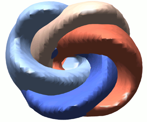
In figure 6, we present isosurfaces of  $0.5\langle \dot {\gamma }\rangle ^*$ and $0.5\langle U \rangle ^*$, the maximum rate of strain and flow velocity, for $Wi= 87$. Figure 6(a–d) show four time steps throughout a circulation, where the volume of high rate of strain forms a band about the circumference of the core of the jet (the pink isosurface). Moreover, the $\langle \dot {\gamma }\rangle ^*$ isosurface extends further upstream on one side of the jet for all time steps, i.e. the rate of strain is greater along one side of the jet. An animated loop of the jet circulating with the rate-of-strain volume is shown in supplementary movie 2. We directly compare the rate of strain forward in time in figure 6(e) as projections of $\langle \dot {\gamma }\rangle ^*$ from (a–d) from the $-x^*$ direction. Moving clockwise from the $\phi ^*=0.12$ isosurface, each surface forward in time presents a decrease in the rate of strain in the clockwise direction or, in other words, a perpetual retreat of the central jet from regions of increased rate of strain. The dynamics of elastic contraction flow has been reported to be sensitive to the extensional rheology (Rothstein & McKinley Reference Rothstein and McKinley2001; Alves & Poole Reference Alves and Poole2007), and since our HPAA solution strain hardens (figure 1c), we can infer from the flow kinematics that the central jet moves about the contraction driven by gradients of strain-hardening HPAA, which will tend to follow the regions of increased rate of strain. This sheds new light onto the likely significance of extensional rheology for local dynamics in viscoelastic contraction flow, as experimentally describing flow topology via directly resolving the rate-of-strain tensor has not been achieved hitherto for elastic flow instability.

Figure 6. (a–d) Phase-averaged isosurfaces of  $0.5\langle \dot {\gamma }\rangle ^*$ and $0.5\langle U\rangle ^*$ for $Wi= 87$. (e) The $-x^*$ projection of the $\langle \dot {\gamma }\rangle ^*$ surfaces from (a–d), coloured by their normalized phase time $\phi ^*$. For advancing time $\phi ^*$, the inner jet displaces towards decreasing rate of strain.
4. Conclusions
Using  $\mathrm {\mu }$-TPIV, we have experimentally resolved for the first time the highly 3-D dynamics of viscoelastic flow through a square–square microcontraction at low $Re$ and high $Wi$. We captured steady and periodic flow instability for a central jet of fluid passing through a toroidal vortex pinned about the contraction entrance, and observed a new vortex growth plateau where the period of instability decreases with $Wi$ but the enveloped vortex volume stagnates. For low $11\leq Wi\leq 22$, the jet circulates with a symmetric cyclical velocity fluctuation likely originating from geometric imperfections. This region coincides with the vortex growth plateau. At higher $Wi\geq 44$, a strong asymmetry in the jet forms, which corresponds to exiting the growth plateau. This would indicate that the asymmetric mode provides a preferable route to vortex growth. We determined the first experimental mapping of the full rate-of-strain tensor to transient dynamics for viscoelastic flow instabilities. We relate regions of increased rate of strain and the extensional rheology of the fluid to the directionality of the circulating jet. Gradients of strain hardening in the fluid provide a likely circulation mechanism as the jet retreats from locally strain-hardened regions of the flowing viscoelastic polymer solution, allowing us to gain new insight into the significance of extensional rheology to local dynamics of viscoelastic contraction flow.
Supplementary movies
Supplementary movies are available at https://doi.org/10.1017/jfm.2021.620.
Funding
We gratefully acknowledge the support of the Okinawa Institute of Science and Technology Graduate University (OIST) with subsidy funding from the Cabinet Office, Government of Japan. We also acknowledge financial support from the Japanese Society for the Promotion of Science (JSPS, Grant Nos. 21K14080, 18K03958, 18H01135 and 21K03884).
Declaration of interests
The authors report no conflict of interest.


 Open access