


1. Introduction
The omnipresence of fluid–structure systems calls for persistent research and exploration into their fluid mechanics. To date, fluids’ volatility, their nonlinear interactive mechanisms with structures and the unsolved Navier–Stokes equations leave this topic a persisting enigma. Fortunately, recent advancements in data science have offered a brand-new pathway to the solution (Budišić, Mohr & Mezić Reference Budišić, Mohr and Mezić2012; Kutz et al. Reference Kutz, Brunton, Brunton and Proctor2016; Lusch, Kutz & Brunton Reference Lusch, Kutz and Brunton2018; Raissi et al. Reference Raissi, Wang, Triantafyllou and Karniadakis2019). Seven decades after the ingenious Koopman theory (Koopman Reference Koopman1931; Koopman & Neumann Reference Koopman and Neumann1932), its mathematical promise was brought to life by the pioneers of data science (Mezić Reference Mezić2005; Rowley et al. Reference Rowley, Mezić, Bagheri, Schlatter and Henningson2009; Schmid Reference Schmid2010; Mauroy & Mezić Reference Mauroy and Mezić2012). Since then, the Koopman analysis has been pervasively applied to fluid problems with success, with many of them directly involving fluid–structure interactive or reactive systems (Muld, Efraimsson & Henningson Reference Muld, Efraimsson and Henningson2012; Carlsson et al. Reference Carlsson, Carlsson, Fuchs and Bai2014; Magionesi et al. Reference Magionesi, Dubbioso, Muscari and Di Mascio2018; Garicano-Mena et al. Reference Garicano-Mena, Li, Ferrer and Valero2019; Miyanawala & Jaiman Reference Miyanawala and Jaiman2019; Page & Kerswell Reference Page and Kerswell2019; Eivazi et al. Reference Eivazi, Veisi, Naderi and Esfahanian2020; Li, Tse & Hu Reference Li, Tse and Hu2020a,Reference Li, Tse and Hub; Wu, Meneveau & Mittal Reference Wu, Meneveau and Mittal2020; Dotto et al. Reference Dotto, Lengani, Simoni and Tacchella2021; Herrmann et al. Reference Herrmann, Baddoo, Semaan, Brunton and Mckeon2021; Jang et al. Reference Jang, Ozdemir, Liang and Tyagi2021; Li et al. Reference Li, Chen, Tse, Weerasuriya, Zhang, Fu and Lin2021; Reference Li, Chen, Tse, Weerasuriya, Zhang, Fu and Lin2022c,Reference Li, Chen, Tse, Weerasuriya, Zhang, Fu and Lind,Reference Li, Chen, Tse, Weerasuriya, Zhang, Fu and Line; Liu et al. Reference Liu, Li, Hao, Zhang and He2021a,Reference Liu, Long, Wu, Huang and Wangb,Reference Liu, Sun, Yeh, Ukeiley, Cattafesta and Tairac; Chen et al. Reference Chen, Wang, Wang, Huang, Tse, Li and Lin2022; Li, Chen, & Tse Reference Li, Chen and Tse2022b). Several works have summarized the current status of the Koopman analysis in fluid applications and subordinate data-driven algorithms (Mezić Reference Mezić2013; Rowley & Dawson Reference Rowley and Dawson2017; Taira et al. Reference Taira, Brunton, Dawson, Rowley, Colonius, McKeon, Schmidt, Gordeyev, Theofilis and Ukeiley2017; Schmid Reference Schmid2022; Li et al. Reference Li, Chen, Zhang, Tse and Lin2023).
On a celebratory note, we observed that most organized research on the Koopman theory was led by applied mathematicians and focused on algorithmic development (Schmid et al. Reference Schmid, Li, Juniper, Pust, Li, Juniper and Pust2011; Budišić et al. Reference Budišić, Mohr and Mezić2012; Brunton et al. Reference Brunton, Proctor, Kutz and Bialek2016). Analysing the algorithmic output is often left to individual, case-by-case interpretations. The present serial effort aims to highlight Koopmanism's unique potentials for analysing fluid–structure systems—deterministically relating observed structure reactions to their flow excitation origins. In Part 1 (Li et al. Reference Li, Chen, Lin, Weerasuriya, Zhang, Fu and Tse2022a), we proposed the linear-time-invariance (LTI) notion and developed an organized and replicable analytical framework called the Koopman-LTI architecture (see figure 1). With a pedagogical demonstration on the subcritical prism wake (i.e. a rigid, infinitely long prism reacting to fluid excitations) and similarity-matrix dynamic mode decomposition (DMD) algorithm as the Koopman approximator, Part 1 successfully:
(1) generated a sampling independent Koopman linearization that captured all the prominent recurring dynamics. The mean reconstruction error, root-mean-square (r.m.s.) reconstruction error and DMD approximation error of the Koopman modes were all at numerical zeros, O−12, O−9 and O−8, respectively;
(2) disclosed w's trivial role in the convection-dominated free-shear flow, Reynolds stresses’ spectral description of cascading eddies, vortices’ sensitivity to dilation and indifference to distortion, and structure reactions’ origin in vortex activities;
(3) reduced the subcritical wake during shear layer transition II into only six dominant excitation-reaction dynamics. The upstream and crosswind walls constitute a dynamically unified interface, which is dominated by only two mechanisms at St = 0.1242 and St = 0.0497 (Class 1). The downstream wall remains a distinct interface and is dominated by four other mechanisms at St = 0.1739, St = 0.0683, St = 0.1925 and St = 0.2422 (Class 2).

Figure 1. Koopman linear-time-invariance (Koopman-LTI) architecture. It consists of the input curation, Koopman algorithm, linear-time-invariance, constitutive relationship and phenomenological relationship modules. Each module contains several submodules with requirements or options. The Koopman-LTI is purely data-driven, theoretically accommodating all input types and solution algorithms that can accurately approximate the Koopman eigen tuples.
By completing the input curation, Koopman algorithm, linear-time-invariance and constitutive relationship modules, the fluid–structure constitution has been established. The complete analysis essentially comes down to understanding the six mechanisms, which this Part 2 will address through the final phenomenological relationship module.
Phenomenology, the study of phenomena, is the essential path to solution for many fluid–structure systems. As Roshko (Reference Roshko1993) remarked:
‘The problem of bluff body flow remains almost entirely in the empirical, descriptive realm of knowledge.’
In this paper, we propose a methodical improvement, the dynamic Koopman mode, to visualize in-synch, instantaneously varying flow field coherent structures (Hussain Reference Hussain1986) and the corresponding structure reactions, overcoming the phase issues that often trouble static visualizations of the Koopman modes. The newly proposed dynamic Koopman modes also give phenomenological consolidation to spectral fluid–structure constitutions, disclosing the underlying mechanisms and enabling normalizable notions for inter-modal comparisons. In composition, following the introduction here, § 2 analyses the Class 1 mechanisms, § 3 focuses on the Class 2 mechanisms, § 4 presents a newly discovered vortex breathing phenomenon and § 5 offers a summary of the major findings.
2. A brief recapitulation
We briefly present some essential nomenclature and information inherited from Part 1 to facilitate better readability. Figure 1 presents the overall Koopman-LTI architecture, in which this Part 2 focuses exclusively on the final phenomenological relationship section. Table 1 summarizes the ten most dominant eigen tuples for each measurable (highlighted), resulting in precisely 30 across the entire inventory. In total, 18 field and wall measurables have been sampled as independent realizations (see table 2). Readers may find the relevant definitions in Li et al. (Reference Li, Chen, Tse, Weerasuriya, Zhang, Fu and Lin2022c). The subsequent text refers to the upstream (AB), top (BC), downstream (CD) and bottom (DA) walls according to the orientation in figure 2. After Liu (Reference Liu2019), this work also refers to the vorticity-based vortex identification criterion, namely |ω|, as the first-generation vortex field, the eigenvalue-based criteria, namely q and λ 2, as the second-generation, and the ratio-based criteria, namely  $\varOmega$ and $\tilde{\varOmega}_R$, as the third-generation.

Figure 2. Orientation and location of the prism walls.
Table 1. Summary of 30 dominant modes and their respective  $|\tilde{\alpha}_{j}|$ ranking in each Koopman-LTI system (highlighted: 10 most dominant).

Table 2. Summary of the inventory consisting of 18 measurables.

3. Phenomenological relationship (module 5) – Class 1
Before we begin, a limitation of modal visualization is clarified. Like any type of eigen mode shape, a dynamic Koopman mode only illustrates the bin-wise-averaged relationship of its spatiotemporal content, so the fluid–structure correspondence and synchrony are governed by the resolution of spectral discretization, highlighting the criticality of the LTI convergence. For this reason, we limit our discussion to the descriptive, phenomenological realm of fluid mechanics. Even so, as the upcoming sections will demonstrate, the physics embedded in the dynamic modes are already immensely rich. Readers are also reminded that mode shapes only describe the relative relationships between coherent dynamics, meaning the information contained in a mode is quintessentially identical to its opposite-sign counterpart. Therefore, in the subsequent sections, all terms of ‘positive’ and ‘negative’ refer to relative correlations instead of mathematical constitution. According to Lander et al. (Reference Lander, Letchford, Amitay and Kopp2016), we also define the prism base as the streamwise distance between the downstream wall and 2.5D and the near-wake as the after-wake up to 7D. The ensuing discussions are also based on the dynamic Koopman modes, so each static mode shape image is supplemented by a movie file. Please refer to the supplementary material, available at https://doi.org/10.1017/jfm.2023.36, for the reduced-size and full HD files.
3.1. M 1 – shear layer dynamics and Bérnard–Kármán shedding
3.1.1. Pressure field P
We begin with the Class 1 mechanisms. Figure 3 presents the normalized dynamic Koopman mode M 1 (St 1 = 0.1242) of P inside the flow domain and on the walls of the prism. The multimedia file depicts the alternating occurrence, development and shrinkage of separation bubbles adhering to the crosswind walls, as well as the subsequent shedding of coherent wake structures. By frequency-matching, we visualize the in-synch behaviours of the flow field and the corresponding structure reactions.

Figure 3. Normalized dynamic Koopman mode (−1 to 1) M 1 (St 1 = 0.1242) of P inside the flow domain and on the walls of the prism at (a) t* = 0 and (b) t* = 4.49960: iso-surfaces ±0.25 of P (top left); mid-prism-span slice of P (top right); the bottom (DA), upstream (AB), top (BC) and downstream (CD) walls, respectively (bottom from left to right). Multimedia file slowed by a factor of 500.
Specifically, the upstream wall (AB) exhibits consistent morphology throughout the shedding cycle. Only near edges A and B, two slivers of extreme pressure alternate in sign. This is the familiar impression of stagnation and forced separation, as AB of all other Koopman modes show monotonous morphologies with the only difference in the frequency of the sign switch, meeting anticipations and explaining why the upstream wall contains the most stationary dynamics and has the highest growth/decay rate compared to its peers (figure 8 from Part 1).
However, the other three walls’ reactions are dissimilar. The sign-alternating separation bubbles dictate the crosswind reactions. Take the top wall (BC) as an example (see figure 3a). When the bubble is emerging, an intense pressure band forms near the rear edge C (in blue), which is of opposite sign to the upstream (in red). As the bubble forms and grows, the band becomes increasingly weaker. At the maximum bubble intensity, the band becomes like-sign with the upstream and even the high-pressure portions (see figure 3b). Furthermore, the downstream wall (CD) is anti-symmetrically alternating, which is in evident congruence with the bisected architecture of the near-wake. Again, the downstream wall traces back to the behaviours of the separation bubbles, or more, the root in shear layer dynamics.
3.1.2. Velocity magnitude |U|
The velocity field is the most common realization of the flow field and may draw more morphological familiarity to the readers. Figure 4 presents the normalized dynamic Koopman mode M 1 (St 1 = 0.1242) of |U| inside the flow domain and on the walls of the prism. The figure delineates two shear layers stemming off from the leading edges due to forced separation. Their in-synch motion with P confirms the fact that separation bubbles result from the closure circulation zones, which are directly turbulent without a laminar transition (Kiya & Sasaki Reference Kiya and Sasaki1983; Wu et al. Reference Wu, Meneveau and Mittal2020). M 1 also illustrates the shear layers’ dispersion from initially intense wall jets into waning streams as they convect downstream, accompanied by continuous fluid entrainment and vorticity dilution. The shear layers also gain curvature in the process, drawing wake structures increasingly close to the afterbody and toward the downstream wall (figure 3b). The ultimate outcome is the impingement of the leading vortex (Unal & Rockwell Reference Unal and Rockwell1988a,Reference Unal and Rockwellb), also known as reattachment.
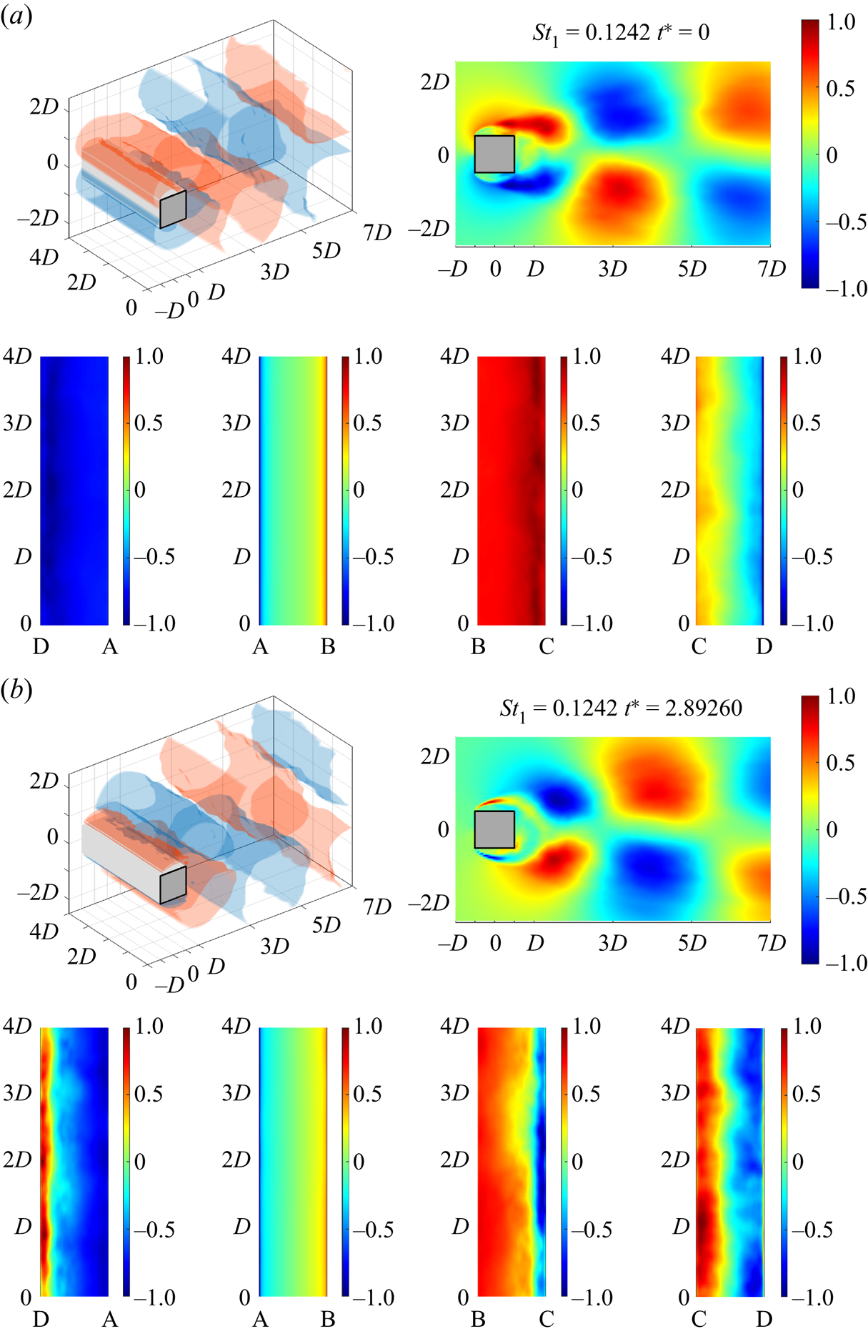
Figure 4. Normalized dynamic Koopman mode (−1 to 1) of M 1 (St 1 = 0.1242) of |U| inside the flow domain and on the walls of the prism at (a) t* = 0 and (b) t* = 2.89260: iso-surfaces ±0.25 of |U| (top left); mid-prism-span slice of |U| (top right); the bottom (DA), upstream (AB), top (BC) and downstream (CD) walls, respectively (bottom from left to right). Multimedia file slowed by a factor of 500.
The aforenoted wall reactions link directly to the shear layers. Taking the top wall (BC) as an example again, the pressure band near C propagates counter-streamwise toward B, through which negative pressure turns to positive in a sharp gradient across 1/5D (see figure 4a). The pressure band results from fluid reversing into the circulating zone, pushing against the forward-traveling mainstream. As the top shear layer disperses and gains curvature, its tendency to close the separation bubble bottlenecks the reverse flow, causing the band to decay in intensity. However, not until the exact moment of bubble closure does the shear layer curvature effectuate into actual reattachment (figure 4b). An immediate consequence is an intra-bubble pressure equalization. The low-pressure band also flips in sign as intense fluid carried by the shear layer impinges onto the wall upon reattachment.
The downstream wall (CD) also shows evidence of reattachment. A bisecting pressure band is observed, which separates the reaction pattern into two spanwise antisymmetric, opposite-sign halves. The two halves’ intense pressures persist throughout the mode's periodicity and are only temporarily relieved as the wake structures cut off their turbulent sheets with the upstream (Sarpkaya Reference Sarpkaya1979). Only at the exact moment of shedding, the two halves rapidly switch signs and restore the pressure bi-polarity (see figure 4b). The pattern results from the curved shear layers approaching the downstream wall, as the sign of the two halves corresponds to that of the respective shear layer.
At this point, it is convenient to summarize the observations of M 1 into a lucid phenomenological process. An asymmetric wall jet resulting from forced, sharp-corner separation develops at the leading edge, shearing the fast external and slow internal fluid as a shear layer. The shear layer gains curvature and momentum thickness due to fluid dispersion and entrainment, both drawing it closer to the afterbody. The strong convection outside the shear layer also add to the curvature gain. The increasing curvature shortens the shear layer's lateral distance to the rear edge, bottlenecks the reverse flow and eventually culminates into reattachment. The reattachment, manifested as the closure of separation bubbles, suppresses the reverse flow altogether and stifles the shear layer's momentum transfer into the wake. Notwithstanding, the halt of momentum outlet is not accompanied by that of generation. As such, momentum continues to build up inside the enclosed bubble, dilating it in all directions. The dilation cannot penetrate the wall; it encounters a strong, incessant resistance from the oncoming free-stream, and an even stronger one from the leading edge jet. With no other option, the bubble's membrane-like structure succumbs to the continuous build-up at the feeblest point – the rear edge, unleashing the pent-up momentum and shedding fluid of coherent patterns into the prism base. This cyclic process was puzzled together after centuries of outstanding research (Nakamura & Nakashima Reference Nakamura and Nakashima1986; Zhao et al. Reference Zhao, Leontini, Lo Jacono and Sheridan2014; Trias, Gorobets & Oliva Reference Trias, Gorobets and Oliva2015; Portela, Papadakis & Vassilicos Reference Portela, Papadakis and Vassilicos2017; Bai & Alam Reference Bai and Alam2018; Lander et al. Reference Lander, Moore, Letchford and Amitay2018; Cao, Tamura & Kawai Reference Cao, Tamura and Kawai2020; Chen et al. Reference Chen, Huang, Tse, Xu and Li2020, Reference Chen, Fu, Xu, Li, Kim and Tse2021, Reference Chen, Zhang, Li, Xue, Zhang, Kim and Li2023; He et al. Reference He, Zhang, Chen and Li2022), and is now effectively isolated and visualized by the Koopman-LTI.
Dissecting |U| into individual velocity components exposes a consistent morphology in u and v, while w appeals to a different mechanism unrelated to the shear layers. Our investigation also supports the overwhelming contribution of u in the total content of |U|, as their dynamic behaviours display close resemblance (see figure 10 from Part 1). The dynamic Koopman modes of M 1 of u, v and w are presented in the Appendix figures 14–16 for concision.
3.1.3. q-criterion
A step forward is to examine vortex structures in the flow field. This paper presents q and  $\tilde{\varOmega}_{R}$ to exemplify the largely self-similar observations obtained from the second- and third-generation vortex criteria. We spare the first-generation because Gao & Liu (Reference Gao and Liu2018) and Jeong & Hussain (Reference Jeong and Hussain1995) made a critical distinction between vorticity and a vortex, deeming |ω| as obsolete. Accordingly, figure 5 presents the normalized dynamic Koopman mode M 1 (St 1 = 0.1242) of q inside the flow domain and on the walls of the prism.

Figure 5. Normalized dynamic Koopman mode (−1 to 1) of M 1 (St 1 = 0.1242) of q inside the flow domain and on the walls of the prism at (a) t* = 0 and (b) t* = 2.89260: iso-surfaces ±0.25 of q (top left); mid-prism-span slice of q (top right); the bottom (DA), upstream (AB), top (BC), and downstream (CD) walls, respectively (bottom from left to right). Multimedia file slowed by a factor of 500.
The most apparent coherent structures are identified alongside the shear layers. They are opposite-sign and outline the shear layers’ momentum thickness, depicting two shearing interfaces between the jet stream and the surrounding flow. This is an elegant picture of the Kelvin–Helmholtz (KH) instability during shear layer transition II (Lander et al. Reference Lander, Letchford, Amitay and Kopp2016, Reference Lander, Moore, Letchford and Amitay2018). We examine the top shear layer as an example. Fluid convects at low or even negative velocities inside the recirculation zone, so intense viscous shearing generates the inner interface as the forward-traveling jet encounters slow/reverse flow, causing the roll-up of the interfacial KH vortices. By contrast, the outer interface results from the jet stream shearing with the corner accelerated, external flow. Expectedly, figure 5 shows that the outer and inner KH vortices have opposite-sign, appropriately describing the relative relationship between the two shearing interfaces. Afterwards, the KH structures convect downstream alongside the curved shear layers. Figure 5(a) lucidly depicts how the rear corner cuts into a shear layer's inner interface, presenting unambiguous evidence of the leading vortex impingement and the destined collision of the KH vortices into the prism wall as the result of reattachment.
On a different note, though q appropriately depicts the KH instability, it fails to identify coherent vortex structures in the wake. The failure reflects the issue that Liu et al. (Reference Liu, Gao, Dong, Wang, Liu, Zhang, Cai and Gui2019) discussed – the eigenvalue-based, second-generation criteria depend highly on the user-defined threshold. Finding an appropriate one that suits both the global and local vortex scales is often difficult, if at all achievable. Threshold prescription is even trickier when the spatiotemporal content is transcribed into the Fourier space by the Koopman analysis. Therefore, though q, or the second-generation criteria in general, has rich information, controlling its threshold can be practically intractable after decomposing data into Koopman eigen tuples.
3.1.4.  $\tilde{\varOmega}_{R}$–criterion

Avoiding the issue of threshold, Figure 6 presents the normalized dynamic Koopman mode M 1 (St 1 = 0.1242) of the third-generation criterion  $\tilde{\varOmega}_{R}$ inside the flow domain and on the walls of the prism. An immediate observation is its resemblance with the velocity field, reaffirming the that the coherent structures observed in §§ 3.1.1 and 3.1.2 indeed result from vortical activities. However, there is an intriguing catch. A comparison of |U| (figure 3b) and $\tilde{\varOmega}_{R}$ (figure 5b) shows the shedding of the primary structures is escorted by an entourage of small-scale vortices. These smaller vortices are scattered in the near wake and do not necessarily conform to the borders of the primary structure. However, as the shedding progresses, the smaller vortices quickly dissipate, and only those within the primary structure survive (figures 3a and 6a). A vortex's rotation acts as the shelter for small coherent structures.

Figure 6. Normalized dynamic Koopman mode (−1 to 1) of M 1 (St 1 = 0.1242) of  $\tilde{\varOmega}_{R}$ inside the flow domain and on the walls of the prism at (a) t* = 0 and (b) t* = 2.89260: iso-surfaces ±0.25 of $\tilde{\varOmega}_{R}$ (top left); mid-prism-span slice of $\tilde{\varOmega}_{R}$ (top right); the bottom (DA), upstream (AB), top (BC) and downstream (CD) walls, respectively (bottom from left to right). Multimedia file slowed by a factor of 500.
On a methodical note, the downside of  $\tilde{\varOmega}_{R}$ is apparent too. The price of a universal threshold is the loss of local details. Though still vaguely visible, $\tilde{\varOmega}_{R}$'s description of the shear layer's momentum thickness is less favourable, let alone the more intricate details of the interfacial KH vortices. To this end, the ratio-based criteria are not, at least for the scopes herein, necessarily an improvement of the eigenvalue-based criteria. It simply lends an alternative lens to examine vortex dynamics.
3.1.5. Broadband content
It shall be noted that the same exhaustive analysis has been conducted for every dynamic Koopman mode, but, for concision, only the most relevant discussions are presented in the subsequence. The less pivotal figures are assorted in the Appendix.
The preceding discussions motivated an examination of the broadband content of the primary mode M 1. The dynamic Koopman modes of M 2 (St 2 = 0.1180) and M 4 (St 4 = 0.1304) of |U| inside the flow domain and on the walls of the prism are presented in the Appendix figures 17 and 18. Analysis corroborates that M 2 and M 4, though less energy-potent, are morphologically identical to M 1, confirming their shared, broadband origin. The observation also extends to several other modes of adjacent frequencies, namely M 8 (St 8 = 0.1428), M 10 (St 10 = 0.1118), M 11 (St 11 = 0.1366), M 12 (St 12 = 0.1056) and M 14 (St 14 = 0.1553). The similitude confirms the conclusion drawn from Part 1, suggesting the broadband content of the primary peak is distributed across several frequency bins within St = 0.1–0.15 (see figure 14(a) from Part 1).
3.1.6. Longitudinal rolls
M 1 and its subsidiaries are related to shear layer dynamics, which result in the Bérnard–Kármán vortex shedding's primary structure – the rolls (Hussain Reference Hussain1986). Originating from forced separation, foreshadowed by fluid dispersion and shear layer curvature, instigated by reattachment and shear layers roll-up (Wu et al. Reference Wu, Sheridan, Hourigan and Soria1996), and supplemented by the intra-shear layer Kelvin–Helmholtz instability (Bloor Reference Bloor1964; Gerrard Reference Gerrard1966; Khor, Sheridan & Hourigan Reference Khor, Sheridan and Hourigan2011), vorticity-infused fluid culminates into the span-wise longitudinal rolls, otherwise known as the Strouhal vortex (Wu et al. Reference Wu, Sheridan, Hourigan and Soria1996).
The Koopman-LTI analysis isolated and pinpointed the structure's reattachment-type reactions due to the rolls. For engineering practice, the reduction of unsteady crosswind lift effectively comes down to the diminution of separation and reattachment. For example, chamfering the leading corners reduces the wall jets’ intensity (Kwok, Wilhelm & Wilkie Reference Kwok, Wilhelm and Wilkie1988), shortening the afterbody length prevents reattachment (Ongoren & Rockwell Reference Ongoren and Rockwell1988; Luo et al. Reference Luo, Yazdani, Chew, & Lee and S1994; Zhao et al. Reference Zhao, Leontini, Lo Jacono and Sheridan2014) and freestream turbulence weakens separation and so the correlations of forces (Vickery Reference Vickery1966; Lee Reference Lee1975; McLean & Gartshore Reference McLean and Gartshore1992; Lyn & Rodi Reference Lyn and Rodi1994). Fascinatingly, based on the preceding analysis, one may infer that chamfering a prism's leading or trailing corners have fundamentally different effects.
3.2. M 5 – turbulence production
3.2.1. Tail-blob substructures
After M 1, this section analyses the secondary mode of Class 1, M 5. Figure 7 presents the normalized dynamic Koopman mode M 5 (St 5 = 0.0497) of P inside the flow domain and on the walls of the prism. The morphology notably differs from that of M 1, in which two main types of wake substructures are observed (also shown by  $\tilde{\varOmega}_{R}$ in the Appendix figure 19). The first, referred to as the tails, depicts the longitudinal, tail-like coherent structures that appear anti-symmetrically about the wake centreline. The tails cover the entire streamwise distance of the near-wake (figure 7a). The second, referred to as the blob, depicts a blob of fluid that adheres to the downstream wall (figure 7b). Interestingly, the tails and blob are separated by an opposite-sign cavity. Structure-wise, reattachment-type reactions are still observed on the crosswind walls. Nonetheless, the downstream wall, instead of the symmetric pattern of M 1, reflects the overwhelming effect of the blob substructure: the negative pressure at mid-span depends directly on the size and intensity of the wall-adhering fluid.
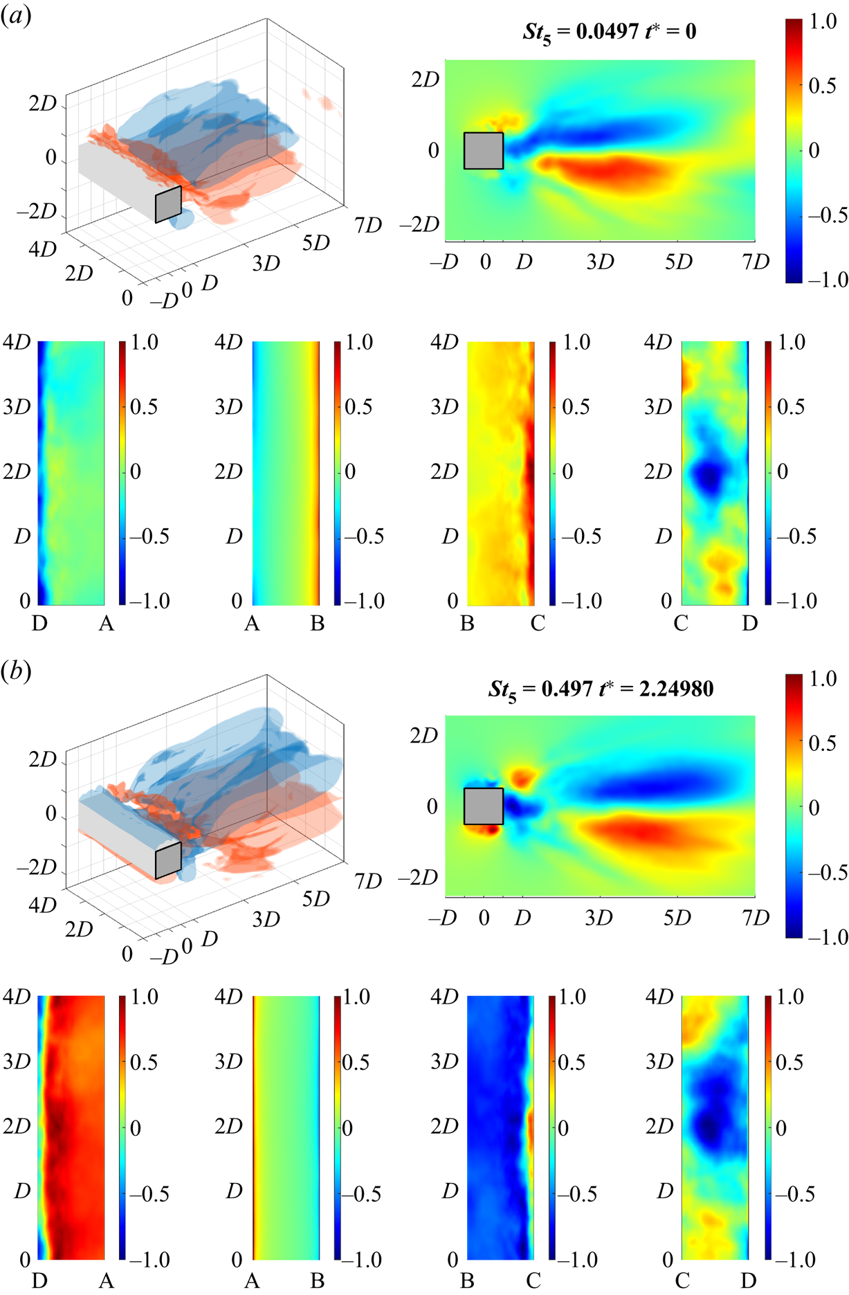
Figure 7. Normalized dynamic Koopman mode (−1 to 1) of M 5 (St 5 = 0.0497) of P inside the flow domain and on the walls of the prism at (a) t* = 0 and (b) t* = 2.24980: iso-surfaces ±0.25 of P (top left); mid-prism-span slice of P (top right); the bottom (DA), upstream (AB), top (BC) and downstream (CD) walls, respectively (bottom from left to right). Multimedia file slowed by a factor of 500.
Apart from P, the normalized dynamic Koopman mode M 5 of |U|, especially figure 8(b), unveils a note-worthy observation – M 5 originates from the shear layers, implying that M 1 and M 5 share origin and are interrelated. After a comprehensive analysis, it is concluded that M 5 describes the mechanisms of turbulence production. The tails are characteristic of the time-averaged production that includes the shear production with sufficient convection. In most turbulent free-shear flows, the mean velocity gradient and the mean momentum transfer are like-sign, resulting in a positive production and generation of the tail structures. This was originally observed by Hussain (Reference Hussain1986) on turbulent jets (figure 9a).

Figure 8. Normalized mode shapes (−1 to 1) of M 5 (St 5 = 0.0497) of |U| inside the flow domain and on the walls of the prism (a) t* = 0 and (b) t* = 2.24980: iso-surfaces ±0.25 of |U| (top left); mid-prism-span slice of |U| (top right); the bottom (DA), upstream (AB), top (BC) and downstream (CD) walls, respectively (bottom from left to right). Multimedia file slowed by a factor of 500.

Figure 9. (a) Contour of time-averaged production and negative production (dotted) showing coherent structures in the near field of an axisymmetric jet at the instant of pairing in the jet column mode at x ≈ 1.75D. Image taken from figure 3 of Hussain (Reference Hussain1986). (b) Direct numerical simulation (top left) and a schematic illustration (top right) of rib–roll dynamics; flow details around a saddle (bottom left) and a more realistic picture of ribs and rolls. Image taken from figure 12 of Hussain (Reference Hussain1986).
3.2.2. Turbulence production in the prism wake
If one considers the prism wake as two stacked mixing layers or asymmetric wall jets, then the antisymmetric twin tail morphology comes as no surprise. However, the shear layers’ non-symmetry brings about the issue of negative production, in which the zeros of the mean velocity gradient and the mean momentum transfer do not always coincide. The incongruence produces small regions where the mean velocity gradient and the mean momentum transfer are opposite-sign (figure 8a). The appearance of the cavity in figure 7(b) is precisely due to the negative production. The dynamic Koopman mode animates the cavity's gradual formation and intrusion into the originally one-piece structure, breaking it apart into the near-wake tail and wall-adhering blob substructures.
The source of turbulence production is vortex stretching and fluid entrainment. According to the serial work of Hussain, a substructure, known as ribs, arises from the stretching of the primary longitudinal rolls (Hussain & Zaman Reference Hussain and Zaman1980; Hussain Reference Hussain1981, Reference Hussain1986; Hussain & Hasan Reference Hussain and Hasan1985). While the shear layers continuously deposit vorticity into the rolls (the process illustrated by M1), the ribs wrap around them in a helical fashion to enrich the longitudinal core's spanwise content. Vortex stretching drives the incessant entrainment of irrotational fluid into the vortex structures, and the location of fluid mixing is precisely at the rib–roll interface. This rib–roll entrainment process is like how a helically ribbed shaft rotates and draws meat into a meat grinder. As the shear layer curves towards the prism base, the negative production isolates the blob from the tail. Consequently, the rib–roll helix is imprinted onto the downstream wall, causing a staggered pattern in which the separatrix of the ribs separates the positive and negative regions (see figure 8b).
In sum, one may trace the shared origin of the Class 1 mechanisms, namely M 1 and M 5, to the shear layer dynamics, the associated Bérnard–Kármán shedding and turbulence production. Class 1 corresponds to the most natural, energetic flow field structures that dominate the reactions of the on-wind wall. Their similarity in dynamical content also renders the three on-wind walls as a spectrally coupled fluid–structure interface, despite their geometric differences. However, the role of vortex stretching in turbulence production can be summarized as the consistent thinning (on statistical average) of fluid elements in the direction perpendicular to the stretching, reducing the radial length scale of the associated vortical structures and ultimately driving the downward cascade into the dissipative scales.
4. Phenomenological relationship (module 5) – Class 2
While the Class 1 mechanisms overwhelm the on-wind walls, their influence on the downstream wall is far from a monopoly. Part 1 identified four ancillary peaks at St 3 = 0.2422 (M3), St 7 = 0.0683 (M7), St 9 = 0.1739 (M9) and St 13 = 0.1925 (M13), which overshadow the downstream wall. This section will analyse the phenomenology of the Class 2 mechanisms.
4.1. M 3 – second harmonic
To begin, figure 10 presents the normalized dynamic Koopman mode M 3 (St 3 = 0.2422) of |U| inside the flow domain and on the walls of the prism. The coherent structures are typical of the widely reported harmonic excitation (Ducoin, Loiseau & Robinet Reference Ducoin, Loiseau and Robinet2016; Kutz et al. Reference Kutz, Brunton, Brunton and Proctor2016). It is also well known that the development of turbulence links closely to spatiotemporal wavefronts (Sengupta, Rao & Venkatasubbaiah Reference Sengupta, Rao and Venkatasubbaiah2006; Sengupta & Bhaumik Reference Sengupta and Bhaumik2011; Bhaumik & Sengupta Reference Bhaumik and Sengupta2014), so the detection of harmonics supports the investigation's correctness. The frequency St 3–2St 1 confirms M 3 is the second harmonic. Though spared from presentation, we also identified higher harmonics like the third harmonic M 16 (St 16 = 0.3664) St 16–3St 1. M 3 plays a significant role in the spatiotemporal composition of the flow field (ranks the 4th in table 1) and the downstream wall (ranks the 9th), but its impacts on the on-wind walls are peripheral (ranks the 14th, 13th and 19th for BC, DA and AB, respectively). The observation substantiates a rudimentary principle – a dominant flow field mechanism does not necessarily incite strong reactions from the structure. Even after the global linearization optimally eliminated nonlinearities, the mechanisms of fluid–structure reactions/interactions are still perplexingly entwined.

Figure 10. Normalized mode shapes (−1 to 1) of M 3 (St 3 = 0.2422) of |U| inside the flow domain and on the walls of the prism at (a) t* = 0 and (b) t* = 1.92840: iso-surfaces ±0.25 of |U| (top left); mid-prism-span slice of |U| (top right); the bottom (DA), upstream (AB), top (BC) and downstream (CD) walls, respectively (bottom from left to right). Multimedia file slowed by a factor of 500.
As expected, the crosswind walls display the reattachment-type reactions, conforming to its harmonic lineage. The downstream wall displays a twin-band pattern instead of the mono-band structure of M 1. For example, in figure 10(a), the negative pressure resides in the midspan, and the positive pressures appear near edges C and D. The opposite pressures are separated by two symmetric bands, doubling that of the fundamental mode in echo of the second harmonic. The structure reaction results from an axis-centric wake structure, which detaches the downstream wall starting from the midspan while its two legs linger on the rear edges. This arc oval shape induces a midspan suction with two positive-pressure zones near the edges (see figure 10a).
4.2. M 7 – subharmonic
Next, figure 11 presents the normalized dynamic Koopman mode M 7 (St 7 = 0.0683) of |U| inside the flow domain and on the walls of the prism. Aside from their frequency, M 7 and M 3 exhibit striking similarities. M 7, too, originates from the shear layers. Its coherent structures are axis-centric about the wake centreline (particularly evident in P in the Appendix figure 20). Like M 3, M 7 also has a considerable role in the flow field (ranks the 8th) and the downstream wall (ranks the 6th), but only triggers lukewarm reactions from the on-wind walls (ranks the 11th, 21st and 17th for BC, DA and AB, respectively), The indifference of the on-wind walls (or the susceptibility of the downstream wall) to Class 2 mechanisms is in sharp contrast with the Class 1 mechanisms, supporting the shared lineage of M 7 and M 3. For its frequency St 7–0.5St 1, M 7 is the subharmonic of the primary structure M 1. Our analysis also discovered that M 6 (St 6 = 0.0745) is the broadband twin of M 7, whose mode shape is merely opposite-sign (Appendix figures 21 and 22). Ducoin et al. (Reference Ducoin, Loiseau and Robinet2016) also made similar observations on the subharmonic peak in the wake of an SD7003 airfoil.

Figure 11. Normalized mode shapes (−1 to 1) of M 7 (St 7 = 0.0683) of |U| inside the flow domain and on the walls of the prism at (a) t* = 0 and (b) t* = 4.49960: iso-surfaces ±0.25 of |U| (top left); mid-prism-span slice of |U| (top right); the bottom (DA), upstream (AB), top (BC) and downstream (CD) walls, respectively (bottom from left to right). Multimedia file slowed by a factor of 500.
4.3. M 9 – ultra-harmonic
After pinpointing the second harmonic M 3, third harmonic M 16 and subharmonic M 7, a natural next step is to search for the ultra-harmonic: M 9 is located with a frequency St 9–1.5St 1. Figure 12 presents the normalized dynamic Koopman mode M 9 (St 7 = 0.1739) of P inside the flow domain and on the walls of the prism, illustrating the axis-centric and sequential arrangement of the coherent structures (also |U| in the Appendix figure 23). As anticipated, the downstream wall is again acutely sensitive to the excitation of the ultra-harmonic. M 9, ranking only the 11th in the flow field dominance, generates the 2nd most impactful Class 2 reaction on the downstream wall.

Figure 12. Normalized mode shapes (−1 to 1) of M 9 (St 9 = 0.1739) of P inside the flow domain and on the walls of the prism at (a) t* = 0 and (b) t* = 1.92840: iso-surfaces ±0.25 of P (top left); mid-prism-span slice of P (top right); the bottom (DA), upstream (AB), top (BC) and downstream (CD) walls, respectively (bottom from left to right). Multimedia file slowed by a factor of 500.
Class 2 mechanisms root from harmonic excitation and are responsible for complicated patterns on the downstream wall. The similarity between M 3, M 7 and M 9 unilaterally:
(1) originate from the shear layers with a clear connection to the Class 1 mechanisms (i.e. development of turbulence);
(2) form inside the prism base (<2.5D) where negative base pressure is incurred; and
(3) remain axis-centric as coherent structures convect downstream.
4.4. M 13 – 2P mode
At last, figure 13 presents the normalized dynamic Koopman mode M 13 (St 13 = 0.1935) of P inside the flow domain and on the walls of the prism. M 13 resembles the other harmonics by dominating dynamics on the downstream wall, but fundamentally differs because its coherent structures are not axis-centric. Instead, two parallel, antisymmetric sequences form on either side of the wake axis. The reaction M 13 instigated on the downstream wall is also different from its harmonic peers. The mono-band picture appeals to that of the primary structure M 1 (also  $|U|$ in the Appendix figure 24).

Figure 13. Normalized mode shapes (−1 to 1) of M 13 (St 13 = 0.1925) of P inside the flow domain and on the walls of the prism at (a) t* = 0 and (b) t* = 2.89260: iso-surfaces ±0.25 of P (top left); mid-prism-span slice of P (top right); the bottom (DA), upstream (AB), top (BC) and downstream (CD) walls, respectively (bottom from left to right). Multimedia file slowed by a factor of 500.
To rationalize M 13, we look into its morphology. Three opposite-sign pairs are found in the wake between 0 and 5D. In the same region, only two opposite-sign pairs are found for M 1. Considering its frequency St 13–1.5St 1, M 13 is likely a second ultra-harmonic of the fundamental structure. However, unlike the axis-centric sequence of M 9, the bi-sequential layout of M 13 suggests its strong connection with the Kármán street.
M 13's morphology alludes to the 2P mode originally observed in the wake of a vibrating cylinder after surpassing the initial branch (Williamson Reference Williamson1996; Williamson & Govardhan Reference Williamson and Govardhan2004). As described by Williamson & Roshko (Reference Williamson and Roshko1988), the 2P transition is incited when a cylinder's crosswind motion surpasses a critical value, generating a phase difference between two sub-vortices in a single shedding cycle. The phase difference prevents like-sign vortex amalgamation, and hence 2-Pairs (2P) of vortices instead of 2-Single (2S) ones form in the Kármán street. On this note, we must highlight the differences between the test subject in Williamson & Roshko (Reference Williamson and Roshko1988) and herein, which are aeroelastic versus stiff, and cylinder versus prism.
Nevertheless, is it possible that the 2P mode is a natural ultra-harmonic structure of the bluff body wake? One may rationalize how an oscillating cylinder generates phase differences in the Bérnard–Kármán vortex shedding: lacking sharp edges, a cylinder must rely on crosswind motions to prematurely break the turbulent sheet before vortex amalgamation. If the motions are not substantial enough, the wake remains in the preferred 2S state. However, in the reference frame of the cylinder, the only difference between a rigid and vibrating cylinder is the curvature of the shear layers, such that the greater the oscillation, the more curved the shear layers and the earlier the reattachment.
What if other mechanisms can enhance the curvature for premature reattachment to the same effect? The shortening of the formation length with Re is widely known for the prism wake (Gerrard Reference Gerrard1966; Williamson & Govardhan Reference Williamson and Govardhan2004), which is indeed due to increasingly curved shear layers. Compared to a curvilinear cylinder, a prism's sharp edges can incisively cut turbulent sheets when reattachment takes place. This means structure oscillation, as a way to encourage vortex shedding, is substitutable by sharp edges, nurturing a possibility for the premature shedding of phase-shifted vortices. If so, the 2P shedding in the rigid prism wake becomes spectrally embedded dynamics. Finally, the layouts of the other harmonics display a striking resemblance with that of the 2S mode (Williamson & Govardhan Reference Williamson and Govardhan2004; Morse & Williamson Reference Morse and Williamson2009) – axis-centric, alternating and vividly mono-sequential. Despite the phenomenological inferences, this topic demands further investigations.
5. New phenomenon: vortex breathing
At this point, the origins of the six dominant excitation-reaction mechanisms have been underpinned. The dynamic Koopman modes described the prism wake phenomenology with accuracy and insights. This paper also demonstrated the methodical procedure to arrive at the conclusions, which is replicable to other flows. One may also extend the conclusions to practical benefit: users can now target a specific fluid phenomenon to eliminate an undesired structural reaction. For example, one can use a splitter plate to prevent the axis-centric harmonic excitations, thus eliminating pressure extremities on the downstream wall and weaken turbulence development in the wake (Unal & Rockwell Reference Unal and Rockwell1988b; Song et al. Reference Song, Hu, Tse, Li and Kwok2017).
In light of the preceding discussions, a new phenomenon was discovered. We detected an intriguing feature of the detached wake structures via dynamic visualization. Take the multimedia file of figure 3 as an example, the coherent structures decay in intensity immediately after breaking their turbulent sheets with the separation bubbles. The decay, manifested as the contraction of the iso-surfaces and fading of colour between D and 3D, is dissipation-wise natural and fully expected. However, surprisingly, these structures expand in size and grow in intensity between 3D and 5D. This contraction-expansion motion repeats itself as if the vortices are inhaling and exhaling, and hence the vortex breathing.
The vortex breathing is fascinatingly perplexing because it disobeys intuitions. On a global scale, the total energy decays when all the modes are added together. Yet, for a single mode, if the initial intensity decay is related to the inter-molecular viscous dissipation, then what mechanisms account for the subsequent growth? After inspection, the breathing phenomenon is attributed to the energy exchange in and out of the discrete frequency bins. Given disparities in periodicity, the inhale of one Koopman mode corresponds to the exhale of some others. This exchange of modal energy is an accurate reflection of the wake's dynamic nature. A vortex's downstream convection incessantly injects vorticity into the irrotational fluid in its path, reeling them into circulation. It, too, constantly deposits viscously dissipated fluid in its trail. Therefore, there is a constant energy exchange in the circulation-entrainment-deposition process, which is captured by the energy in and out of a specific eigenfrequency. The onset, development and dissipation of turbulence also conform to spatiotemporal wavefronts, which certainly involve periodic/harmonic exchanges of energy. This also explains why sinusoids are excellent descriptors of the wake dynamics (see figure 8 in Part 1). The local, mode-wise vortex breathing phenomenon also calls for thoughts on its link to the energy cascade – the globally downward trend that permits inverse energy transfer (i.e. inverse cascade) on the local scale.
On a methodical note, vortex breathing demonstrates the importance of the dynamic Koopman mode. From figures 3(a) and 3(b) alone, the coherent structures between 3D and 5D appear, and quite naturally, less intense, less compact and more dispersed compared to their successors between D and 3D. The breathing motion would have been overlooked by a static Koopman mode. Conversely, a logical explanation would have been extremely difficult if the static snapshot was taken at the moment of exhaling, in which the downstream vortex appears more energetic. Dynamics of acute spatiotemporal sensitivity could have also been easily overlooked by static images due to the issue of phase.
6. Conclusions
This serial effort proposed a linear-time-invariance (LTI) notion, or the Koopman linearly time-invariant (Koopman-LTI) modular architecture, to associate fluid excitations and structure reactions. The LTI models reduced the pedagogical prism wake in the shear layer transition II to six dominant excitation-reaction mechanisms in Part 1. This Part 2 dynamically visualized the Koopman modes and unveiled new insights into the phenomenology of the prism wake. Specifically, two dynamic Koopman modes at St 1 = 0.1242 and St 5 = 0.0497 describe shear layer dynamics, Bérnard–Kármán shedding and turbulence production, which overwhelm the upstream and crosswind walls by the instigating reattachment-type of reactions. The dynamical similarity of the three walls also means they can be treated as a spectrally unified fluid–structure interface, despite their geometric disparity. Another four harmonic counterparts, namely the subharmonic at St 7 = 0.0683, the second harmonic at St 3 = 0.2422 and two distinct ultra-harmonics at St 7 = 0.1739 and St 13 = 0.1935, dominate the downstream wall and only marginally affect the others. The 2P wake mode is also observed as an embedded harmonic of the bluff-body wake. This work also methodically proposed the dynamic Koopman mode, through which the vortex breathing phenomenon was discovered, which describes the constant and periodic energy exchanges in wake's circulation-entrainment-deposition processes and turbulence development.
Supplementary movies
Supplementary movies are available at https://doi.org/10.1017/jfm.2023.36.
The original HD videos including those from the Appendix can be found at: https://drive.google.com/drive/folders/1AHdhUdAfNwlC1XUh-74PgQWW6jUHXJ5j?usp?=?sharing
Acknowledgements
We give a special thanks to the IT Office of the Department of Civil and Environmental Engineering at the Hong Kong University of Science and Technology. Its support for installing, testing and maintaining our high-performance servers is indispensable for the current project.
Funding
The work described in this paper was supported by the Research Grants Council of the Hong Kong Special Administrative Region, China (Project Nos. 16207719 and 16211821), the Fundamental Research Funds for the Central Universities of China (Project No. 2022CDJXY-016), the National Natural Science Foundation of China (Project Nos. 51908090, 42175180 and 74110-41030203), the Natural Science Foundation of Chongqing, China (Project No. 2022NSCQ-JQX2377), and the Key Project of Technological Innovation and Application Development in Chongqing (Project Nos. CSTB2022TIAD-KPX0145 and CSTB2022TIAD-KPX0142).
Declaration of interests
The authors report no conflict of interest.
Availability of data and material
The datasets generated during and/or analysed during the current work are restricted by provisions of the funding source but are available from the corresponding author on reasonable request.
Code availability
The custom code used during and/or analysed during the current work are restricted by provisions of the funding source.
Author contributions
C.Y.L and Z.C. contributed equally to this work. All authors contributed to the study conception and design. Funding, project management and supervision were led by T.K.T.T. and Z.C. and assisted by X.Z. Material preparation, data collection and formal analysis were led by C.Y.L. and Z.C., and assisted by A.U.W., Y.F. and X.L. The first draft of the manuscript was written by C.Y.L. and all authors commented on previous versions of the manuscript. All authors read, contributed and approved the final manuscript.
Compliance with ethical standards
All procedures performed in this work were in accordance with the ethical standards of the institutional and/or national research committee and with the 1964 Helsinki declaration and its later amendments or comparable ethical standards.
Consent to participate
Informed consent was obtained from all individual participants included in the study.
Consent for publication
Publication consent was obtained from all individual participants included in the study.
Appendix
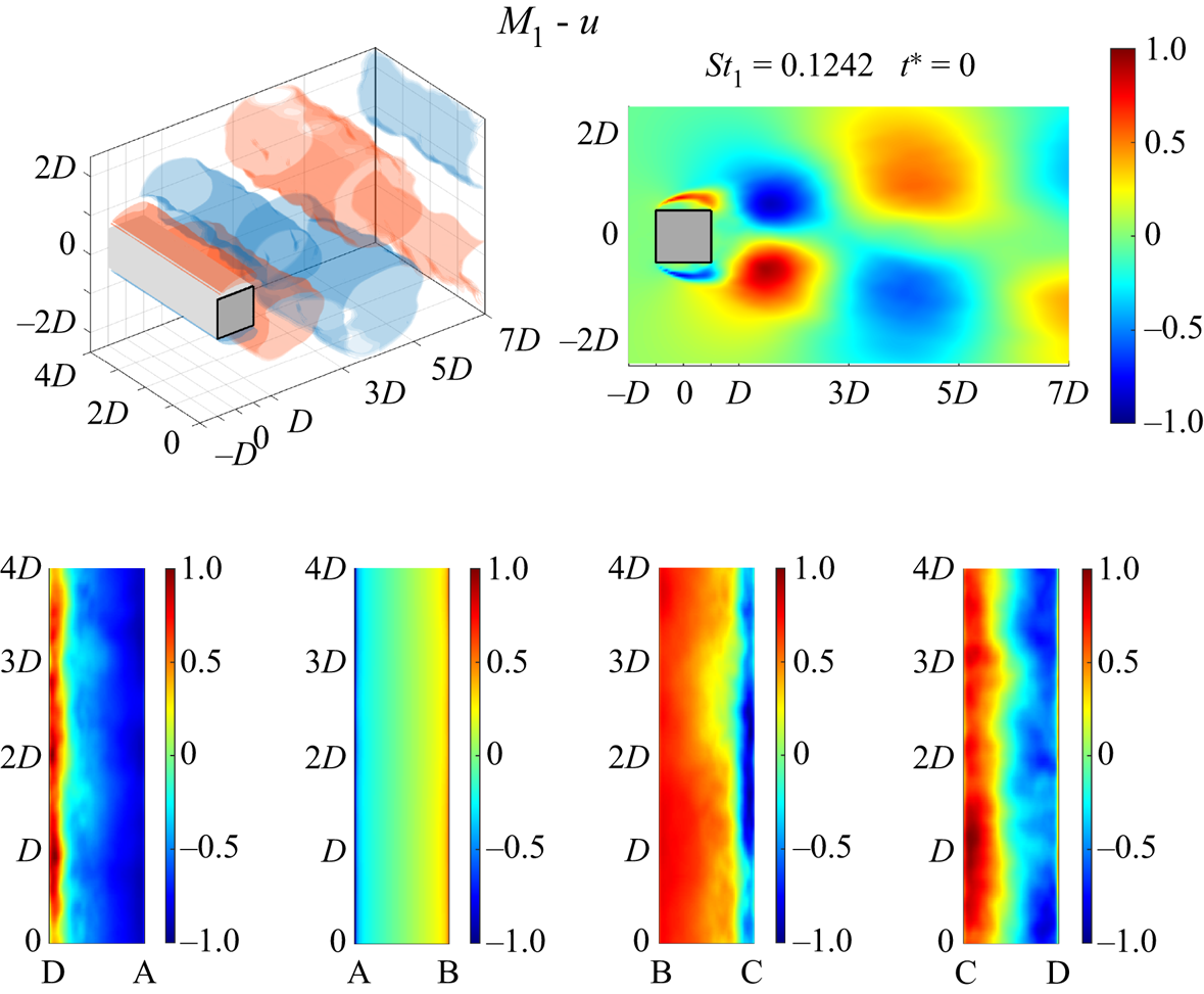
Figure 14. Normalized mode shapes (−1 to 1) of M 1 (St 1 = 0.1242) of u inside the flow domain and on the walls of the prism: iso-surfaces ±0.25 of u (top left); mid-prism-span slice of u (top right); the bottom (DA), upstream (AB), top (BC) and downstream (CD) walls, respectively (bottom from left to right). Multimedia file slowed by a factor of 500.

Figure 15. Normalized mode shapes (−1 to 1) of M 1 (St 1 = 0.1242) of v inside the flow domain and on the walls of the prism: iso-surfaces ±0.25 of v (top left); mid-prism-span slice of v (top right); the bottom (DA), upstream (AB), top (BC), and downstream (CD) walls, respectively (bottom from left to right). Multimedia file slowed by a factor of 500.

Figure 16. Normalized mode shapes (−1 to 1) of M 1 (St 1 = 0.1242) of w inside the flow domain and on the walls of the prism: iso-surfaces ±0.25 of w (top left); mid-prism-span slice of w (top right); the bottom (DA), upstream (AB), top (BC) and downstream (CD) walls, respectively (bottom from left to right). Multimedia file slowed by a factor of 500.

Figure 17. Normalized mode shapes (−1 to 1) of M 2 (St 2 = 0.1180) of |U| inside the flow domain and on the walls of the prism: iso-surfaces ±0.25 of |U| (top left); mid-prism-span slice of |U| (top right); the bottom (DA), upstream (AB), top (BC) and downstream (CD) walls, respectively (bottom from left to right). Multimedia file slowed by a factor of 500.

Figure 18. Normalized mode shapes (−1 to 1) of M 4 (St 4 = 0.1304) of |U| inside the flow domain and on the walls of the prism: iso-surfaces ±0.25 of |U| (top left); mid-prism-span slice of |U| (top right); the bottom (DA), upstream (AB), top (BC) and downstream (CD) walls, respectively (bottom from left to right). Multimedia file slowed by a factor of 500.

Figure 19. Normalized mode shapes (−1 to 1) of M 5 (St 5 = 0.0497) of  $\tilde{\varOmega}_{R}$ inside the flow domain and on the walls of the prism: iso-surfaces ±0.25 of $\tilde{\varOmega}_{R}$ (top left); mid-prism-span slice of $\tilde{\varOmega}_{R}$ (top right); the bottom (DA), upstream (AB), top (BC) and downstream (CD) walls, respectively (bottom from left to right). Multimedia file slowed by a factor of 500.

Figure 20. Normalized mode shapes (−1 to 1) of M 7 (St 7 = 0.0683) of P inside the flow domain and on the walls of the prism: iso-surfaces ±0.25 of P (top left); mid-prism-span slice of P (top right); the bottom (DA), upstream (AB), top (BC) and downstream (CD) walls, respectively (bottom from left to right). Multimedia file slowed by a factor of 500.

Figure 21. Normalized mode shapes (−1 to 1) of M 6 (St 6 = 0.0745) of |U| inside the flow domain and on the walls of the prism: iso-surfaces ±0.25 of |U| (top left); mid-prism-span slice of |U| (top right); the bottom (DA), upstream (AB), top (BC) and downstream (CD) walls, respectively (bottom from left to right). Multimedia file slowed by a factor of 500.

Figure 22. Normalized mode shapes (−1 to 1) of M 6 (St 6 = 0.0745) of P inside the flow domain and on the walls of the prism: iso-surfaces ±0.25 of P (top left); mid-prism-span slice of P (top right); the bottom (DA), upstream (AB), top (BC) and downstream (CD) walls, respectively (bottom from left to right). Multimedia file slowed by a factor of 500.

Figure 23. Normalized mode shapes (−1 to 1) of M 9 (St 9 = 0.1739) of |U| inside the flow domain and on the walls of the prism: iso-surfaces ±0.25 of |U| (top left); mid-prism-span slice of |U| (top right); the bottom (DA), upstream (AB), top (BC) and downstream (CD) walls, respectively (bottom from left to right). Multimedia file slowed by a factor of 500.

Figure 24. Normalized mode shapes (−1 to 1) of M 13 (St 13 = 0.1925) of |U| inside the flow domain and on the walls of the prism: iso-surfaces ±0.25 of |U| (top left); mid-prism-span slice of |U| (top right); the bottom (DA), upstream (AB), top (BC) and downstream (CD) walls, respectively (bottom from left to right). Multimedia file slowed by a factor of 500.


 Open access