


1 Introduction
It is well known that there exists a periodic oscillatory disturbance denoted ‘flapping’ in planar laminar jets. Sato & Sakao (Reference Sato and Sakao1964) made a detailed investigation of the jet flapping using hot-wire anemometry by introducing a controlled sound excitation. They confirmed that the linear theory by Tatsumi & Kakutani (Reference Tatsumi and Kakutani1958) quantitatively predicts the growth of the flapping. Existence of large-scale motions in a turbulent planar jet, similar to the flapping motion, has also been suggested based on two-point velocity correlation measurements (Goldschmidt & Bradshaw Reference Goldschmidt and Bradshaw1973; Cervantes de Gortari & Goldschmidt Reference Cervantes de Gortari and Goldschmidt1981; Antonia et al. Reference Antonia, Browne, Rajagopalan and Chambers1983) although other studies seem to prefer describing these as large-scale coherent structures (Mumford Reference Mumford1982; Thomas & Goldschmidt Reference Thomas and Goldschmidt1986). Such structures have also been extracted by proper orthogonal decomposition (Gordeyev & Thomas Reference Gordeyev and Thomas2000, Reference Gordeyev and Thomas2002).
Large-scale coherent motions have, however, been observed not only in planar jets, but also in other turbulent free shear flows, such as axisymmetric jets, wakes and mixing layers. The reader is referred to Wygnanski & Petersen (Reference Wygnanski and Petersen1987) for a more general discussion of such flows and also the use of linear stability theory to predict the flow development. The concept of coherent structures has been used to provide an estimate on flow properties such as mean velocities, velocity fluctuations and turbulent statistics, but also to understan the interaction between large- and small-scale turbulence. However, in most turbulent flows the structures appear randomly and come in different shapes and phases and are therefore difficult to detect. One of the methods to circumvent this is by imposing a deterministic initial forcing. If the phase of the induced structures is fixed, a phase-average technique can be utilised to educe these structures in a turbulent environment.
In the present study, a nominally two-dimensional jet issuing from a long rectangular channel with large aspect ratio, where the turbulent channel flow is fully developed, was studied. The flow was investigated with hot-wire anemometry using an X-type probe to measure the streamwise and transverse velocity components. A deterministic initial forcing was introduced at the jet outlet and velocity data were phase averaged to extract the large-scale motion. The present experiments differ from most other previous work on two-dimensional turbulent jets in two respects. Most of the investigated jet flows originate from a nozzle, except for the work of Hussain & Clark (Reference Hussain and Clark1977), who studied a jet issuing from a fully developed channel flow. In the nozzle case, the initial jet has a mean velocity profile that is close to ‘top-hat’ and the turbulence level is low. Furthermore, the flow structures usually develop freely; i.e. there is no deterministic forcing. With the present experimental set-up, it is found that the outflowing jet (without the forcing) does not produce any distinct periodic dominant coherent two-dimensional structures by itself, but with forcing such structures can be found and followed as they propagate downstream.
The objective of this work is threefold: (i) to present new experimental results on the mean flow field of a planar turbulent jet that should be more accurate than those reported earlier due to new and more accurate measurement techniques; (ii) to get a good understanding of the instability and flow-structure development by forcing the structures (as done for instance by Nolle (Reference Nolle1998)) and carrying out a triple decomposition of the velocity signal in order to better elucidate the structural behaviour; and (iii) to see how well linear stability theory can predict the structural development of the jet. In addition a new and unexpected finding was discovered, namely the linear scaling of the higher-order covariances of the random components with the amplitude of the forcing.
The paper is structured as follows. Section 2 reviews the relevant literature with respect to the mean flow development of turbulent plane jet flows as well as studies of coherent structures and stability. Section 3 gives the basic equations for a two-dimensional turbulent jet and states how the mean centreline velocity and the jet thickness vary with downstream distance according to similarity theory. It also gives an approximate expression for the mean velocity profiles as well as the Reynolds shear stress, results that will be compared with the experimental data and will be used in the stability calculations. In § 4 it is shown how the flow field can be decomposed into the mean, the periodic and the random (turbulent) parts and it is demonstrated how transport equations for the fluctuations can be obtained. The perturbation dynamics is studied by means of a linear-stability analysis discussed in § 5. Section 6 briefly describes the experimental set-up and the main results are discussed in § 7, first in terms of the undisturbed velocity field and then in terms of the excited velocity field. A self-similar theory will be developed to scale the phase-average velocity field obtained at different excitation frequencies and it will be tested with both the coherent and incoherent statistics. Linear stability calculations will also be discussed to further support the idea that the educed structure follows linear mechanisms. Finally § 8 discusses the results obtained and their implications.
2 Brief review of earlier work
2.1 Mean flow development of plane turbulent jet flows
There are a number of studies on plane turbulent jets although those for axisymmetric jets are far more numerous. We will not make an extensive review but point out some studies that are pertinent to the present work. We assume steady (in the mean) two-dimensional flow with constant density. Here,  $U+u$ and $V+v$ are the streamwise ( $x$-direction) and transverse ( $y$-direction) velocities, respectively, and uppercase and lowercase letters denote mean and fluctuating components. The two-dimensionality implies that the mean of the spanwise velocity is equal to zero; i.e. $W=0$. One of the important parameters of the jet is its spreading rate, usually calculated as $\unicode[STIX]{x1D6FD}_{1/2}=\text{d}\unicode[STIX]{x1D6FF}_{1/2}/\text{d}x$ where $\unicode[STIX]{x1D6FF}_{1/2}$ is the half-width of the jet, defined as the transverse position where $U(x,\unicode[STIX]{x1D6FF}_{1/2})=U_{c}/2$ and $U_{c}$ is the velocity at the centreline of the jet.
There exists a similarity solution of the plane turbulent jet that was probably first described by Townsend (Reference Townsend1956) and has since then been shown in most text books on turbulent flows; e.g. Tennekes & Lumley (Reference Tennekes and Lumley1972) and Pope (Reference Pope2000). The theory for a self-similar flow development of the jet is based on the thin-shear flow approximation, i.e.  $\unicode[STIX]{x2202}/\unicode[STIX]{x2202}x\ll \unicode[STIX]{x2202}/\unicode[STIX]{x2202}y$ and $V\ll U$ and also that the Reynolds number is high enough such that viscous stresses can be neglected in comparison with turbulent stresses. Two of the major results from the similarity theory is that the width of the jet increases as $x$ and that the centreline velocity decreases as $x^{-1/2}$ (see § 3). When deriving the similarity solution for $U,V$ and $\overline{uv}$ there is one crucial assumption, namely that the turbulent ‘eddy’ viscosity is uniform in the transverse direction and then the only empirical input that is needed for the modelling is the jet spreading rate.
Two early studies using hot-wire anemometry to obtain flow statistics were published in 1965, namely Bradbury (Reference Bradbury1965) and Heskestad (Reference Heskestad1965). The Reynolds number,  $Re$, of the jet, based on jet velocity at the outlet, nozzle width ( $d$) and kinematic viscosity was 30 000 and 34 000, respectively. In both studies some earlier work was also reviewed (e.g. Miller & Comings Reference Miller and Comings1957; der Hegge Zijnen Reference der Hegge Zijnen1958a,Reference der Hegge Zijnenb).
In Bradbury (Reference Bradbury1965) the jet issued in a co-flowing environment, i.e. the jet nozzle was mounted in the test section of a wind tunnel, thereby avoiding low flow velocities and high turbulence levels at the jet boundary, which both are difficult to characterise with standard hot-wire anemometry. Two velocity ratios were used where the outer flow was either 7 % or 16 % of the jet exit velocity. He reports results of the streamwise velocity distribution, and the normal stresses in the streamwise,  $\overline{uu}$, transverse, $\overline{vv}$, and spanwise, $\overline{ww}$, directions as well as the Reynolds shear stress, $\overline{uv}$. (Normal and shear stresses are, of course, defined as $-\unicode[STIX]{x1D70C}\overline{uu},-\unicode[STIX]{x1D70C}\overline{vv},-\unicode[STIX]{x1D70C}\overline{ww},-\unicode[STIX]{x1D70C}\overline{uv}$, where $\unicode[STIX]{x1D70C}$ is the fluid density, but for brevity we exclude the minus sign and the density when mentioning Reynolds stresses, as suggested by Pope (Reference Pope2000).) Profiles were measured at different downstream positions in the range $22\leqslant x/d\leqslant 70$ and the jet spreading rate was found to be $\unicode[STIX]{x1D6FD}_{1/2}=0.109$. Bradbury states, based on his results for the measured turbulence quantities, that self-similarity (or as he names it, ‘self-preservation’) occurs for $x/d>30$.
The jet in the facility used by Heskestad (Reference Heskestad1965) issued into still air and he measured the same quantities that were measured by Bradbury (Reference Bradbury1965), but further downstream ( $x/d\approx 100$). In contrast to the statement of Bradbury, he concludes that self-similarity is reached for $x/d>65$. The spreading rate $\unicode[STIX]{x1D6FD}_{1/2}$ was given as 0.110; i.e. close to the value obtained by Bradbury. Qualitatively, the Reynolds stress distribution of these two studies are similar, although the results of Heskestad show a larger scatter.
Ten years later a paper by Gutmark & Wygnanski (Reference Gutmark and Wygnanski1976) was published where the Reynolds number was 30 000 and most of the measurements were taken at  $x/d=120$. All measurements were taken using hot-wire anemometry: single, slanted and X-configurations were used. The spreading rate of the jet was given as $\unicode[STIX]{x1D6FD}_{1/2}\simeq 0.1$. Although they present results also for the transverse mean component $V$, these were obtained based on the measurements of $U$ and calculated by using the continuity equation.
Hussain & Clark (Reference Hussain and Clark1977) studied the influence of outlet conditions on the jet development, by letting the jet discharge both from a laminar nozzle and a turbulent channel flow. They found that for the laminar conditions the entrainment was initially larger than for the channel case, which they suggested was due to the instabilities that develop in the shear layer. For the turbulent case, they studied two Reynolds numbers (32 500 and 81 400). The spreading rate was decreasing slightly with increasing Reynolds number and was reported as 0.115 and 0.110, respectively.
In contrast to the previous studies, measurements by Ramaprian & Chandrasekhara (Reference Ramaprian and Chandrasekhara1985) were performed with laser Doppler velocimetry (LDV) and the fluid was water. With the LDV technique, high turbulence intensities and back-flow could be determined and they were also able to measure the transverse velocity, despite its smallness. The Reynolds number in this study was approximately 15 000, and measurements were presented from stations in the range  $x/d=5$ to 60. The spreading rate was found to be $\unicode[STIX]{x1D6FD}_{1/2}=0.11$. They also provide tables with other studies showing various properties that have been measured. Overall they conclude that the distributions of the Reynolds stresses are qualitatively similar to the earlier studies using hot-wire anemometry but in general the magnitude is smaller.
The effect of Reynolds number on the jet behaviour was studied by Deo, Mi & Nathan (Reference Deo, Mi and Nathan2008). They obtained Reynolds numbers in the range 1500 to 16 500 in their experimental set-up. The measurements were performed with hot-wire anemometry. There was a clear tendency of a decreasing spreading rate with increasing  $Re$, at the highest $Re$ they found $\unicode[STIX]{x1D6FD}_{1/2}\approx 0.09$. They suggested that at least part of this trend is due to different outlet profiles of the two-dimensional jet. In a later work, Deo, Nathan & Mi (Reference Deo, Nathan and Mi2013) showed the distribution of $\overline{uu}$ for various $Re$ and how it developed in the downstream direction.
When it comes to the distribution of  $\overline{uu}$, $\overline{vv}$ and $\overline{uv}$ across the jet, one should also mention the work by Gordeyev & Thomas (Reference Gordeyev and Thomas2000) who show the distribution for various $x/d$ in the range 20 to 90 at $Re=28\,000$. It is interesting to note that these results show clearly lower magnitudes of the stresses than those of Gutmark & Wygnanski (Reference Gutmark and Wygnanski1976). Finally a recent paper by Cafiero & Vassilicos (Reference Cafiero and Vassilicos2019) questions the usual self-similarity solution. Although practically the differences are small it is an interesting contribution. Moreover their measurements of the Reynolds shear stress (and the normal stresses as well) also show lower values as compared to Gutmark & Wygnanski, which seems to indicate that the suitability of those older measurements as the standard for comparison with theory may need to be re-evaluated.
Finally one should also mention that both direct numerical simulations and large-eddy simulations have been used to study the turbulent plane jet. However, in these cases both the length of the domain and the Reynolds number are limiting factors. One of the most recent studies is that of Bisoi et al. (Reference Bisoi, Das, Roy and Patel2017) which also includes an extensive review of earlier numerical simulations of the turbulent planar jet flow.
2.2 Coherent structures in turbulent jet flows
The concept of coherent structures in turbulence is more than 50 years old. Already in the first issue of the Journal of Fluid Mechanics, Donald Coles (Reference Coles1954) makes the hypothesis that a ‘large-eddy structure’ is represented by the wake profile of turbulent boundary layers, meaning that these structures are the building blocks of the mean flow. The interest for coherent structures in turbulence increased over the years as evidenced by an account by Davies & Yule (Reference Davies and Yule1975) of the ‘Colloquium on Coherent Structures in Turbulence’ held in Southampton in March 1974 where at least 45 presentations were given. Here is not the place for a thorough review of the massive amount of work done on coherent structures since then, but we will review some of the research that has dealt with coherent structures related to jet flows.
As mentioned in the introduction, the existence of coherent motion in a turbulent planar jet has been confirmed by correlation measurements using hot wires, for example Mumford (Reference Mumford1982), Antonia et al. (Reference Antonia, Browne, Rajagopalan and Chambers1983) and Thomas & Goldschmidt (Reference Thomas and Goldschmidt1986), and such structures have also been extracted from planar particle image velocimetry (PIV) measurements through proper orthogonal decomposition (Gordeyev & Thomas Reference Gordeyev and Thomas2000, Reference Gordeyev and Thomas2002). In all these cases the jet was developing without any forcing.
There are a few studies of planar laminar jets where linear stability theory has been used to study the evolution of the disturbance. As mentioned in the introduction, the experiments by Sato (Reference Sato1960) and Sato & Sakao (Reference Sato and Sakao1964) confirmed the growth rate of the flapping obtained through linear stability analysis by Tatsumi & Kakutani (Reference Tatsumi and Kakutani1958). There is also more recent experimental and modelling work for low Reynolds number jets by, for example, Nolle (Reference Nolle1998) and Atassi & Lueptow (Reference Atassi and Lueptow2002).
Oberleithner, Rukes & Soria (Reference Oberleithner, Rukes and Soria2014) also studied laminar round jets with planar PIV in water where the flow was driven by a piston in a tube upstream of a contraction. In this set-up the steady piston motion could be overlaid with a sinusoidal variation of various amplitudes (up to 100 % of the piston mean velocity) thereby forcing a disturbance. They decomposed the flow field using proper orthogonal decomposition (POD) and extracted the mean flow distribution. That distribution was evaluated by linear stability analysis which showed convincing agreement with the experimental results.
When it comes to detecting and analysing coherent structures through stability analysis in turbulent jets there are fewer studies available and those available are for round jets. Gudmundsson & Colonius (Reference Gudmundsson and Colonius2011) analysed experimental data from a round jet at high, but subsonic Mach numbers. Velocity data were available from stereo particle image velocimetry (known as S-PIV) and pressure fluctuations from a microphone array. They used both the parabolic stability equation (known as PSE) method and POD to study the disturbance development and concluded that their results indicate that linear theory can be used to predict the largest-scale and most energetic structures if the mean turbulent flow field is used in the analysis. Later on, further studies used linear analyses to investigate the dynamics of wave packets in jets (Garnaud et al. Reference Garnaud, Lesshafft, Schmid and Huerre2013; Cavalieri et al. Reference Cavalieri, Rodríguez, Jordan, Colonius and Gervais2013) with a special focus on the sound produced by the jet (Jordan & Colonius Reference Jordan and Colonius2013).
Oberleithner et al. (Reference Oberleithner, Rukes and Soria2014) and Oberleithner, Paschereit & Soria (Reference Oberleithner, Paschereit and Soria2015) studied an excited turbulent round jet under swirling and no-swirling conditions through both experiments and linear stability analysis. The linear stability analysis was made by using the measured mean flow field and the results showed reasonable agreement with the experiments with respect to the selected mode structure.
Proper orthogonal decomposition was used by Shim, Sharma & Richards (Reference Shim, Sharma and Richards2013) to analyse the initial development of a plane jet at a moderate Reynolds number  $(Re=3000)$. The measurements were done in a water jet flow facility and the velocity data were obtained using planar PIV. The initial jet from the outlet slot had a near top-hat profile and measurements were obtained up to a distance of 9 slot heights. They found initially symmetrical spanwise oriented counter-rotating vortices formed by the shear layer instability on the two sides of the jet, but further downstream they were displaced with respect to each other resulting in the formation of antisymmetrical vortices. This indicates that the most unstable flow structure for the turbulent jet is antisymmetric.
Further discussion and references to works on linear stability analysis in turbulent flows are given in § 5 in the context of the present approach.
3 Basic equations for the two-dimensional turbulent jet
For boundary layers, jets and wakes the thin shear-layer approximation, which assumes that  $x$-derivatives of mean quantities are much smaller than $y$-derivatives and that $V\ll U$, is commonly used. This makes it possible to neglect some terms in the Reynolds averaged Navier–Stokes equations. However, the assumption works better for turbulent boundary layers than for wakes and jets since the spread in the lateral direction is an order of magnitude larger for the latter. However, for jets and wakes a further assumption can be made, namely that for high enough Reynolds numbers, the viscous term can be neglected; see, for instance, Townsend (Reference Townsend1956) and Pope (Reference Pope2000). In order to verify that the thin shear-layer approximation as well as neglecting viscous terms are both valid, these terms can be evaluated a posteriori when the approximate solution has been found. Under the above assumptions the Reynolds-averaged continuity, streamwise ( $x$) and transversal ( $y$) momentum equations reduce to
 $$\begin{eqnarray}\displaystyle & \displaystyle \frac{\unicode[STIX]{x2202}U}{\unicode[STIX]{x2202}x}+\frac{\unicode[STIX]{x2202}V}{\unicode[STIX]{x2202}y}=0, & \displaystyle\end{eqnarray}$$
 $$\begin{eqnarray}\displaystyle & \displaystyle U\frac{\unicode[STIX]{x2202}U}{\unicode[STIX]{x2202}x}+V\frac{\unicode[STIX]{x2202}U}{\unicode[STIX]{x2202}y}=-\frac{1}{\unicode[STIX]{x1D70C}}\frac{\unicode[STIX]{x2202}P}{\unicode[STIX]{x2202}x}-\frac{\unicode[STIX]{x2202}}{\unicode[STIX]{x2202}y}\overline{uv}-\frac{\unicode[STIX]{x2202}}{\unicode[STIX]{x2202}x}\overline{uu}, & \displaystyle\end{eqnarray}$$
 $$\begin{eqnarray}\displaystyle & \displaystyle U\frac{\unicode[STIX]{x2202}V}{\unicode[STIX]{x2202}x}+V\frac{\unicode[STIX]{x2202}V}{\unicode[STIX]{x2202}y}=-\frac{1}{\unicode[STIX]{x1D70C}}\frac{\unicode[STIX]{x2202}P}{\unicode[STIX]{x2202}y}-\frac{\unicode[STIX]{x2202}}{\unicode[STIX]{x2202}y}\overline{vv}-\frac{\unicode[STIX]{x2202}}{\unicode[STIX]{x2202}x}\overline{uv}, & \displaystyle\end{eqnarray}$$
where an overbar denotes the time-average operator.
By assuming that both the left-hand side (LHS) and the  $x$-derivative of the Reynolds shear stress in (3.3) are negligible, it can be integrated to become
 $$\begin{eqnarray}P+\unicode[STIX]{x1D70C}\overline{vv}=P_{\infty },\end{eqnarray}$$
simplifying (3.3) and leading to
 $$\begin{eqnarray}U\frac{\unicode[STIX]{x2202}U}{\unicode[STIX]{x2202}x}+V\frac{\unicode[STIX]{x2202}U}{\unicode[STIX]{x2202}y}=-\frac{1}{\unicode[STIX]{x1D70C}}\frac{\text{d}P_{\infty }}{\text{d}x}-\frac{\unicode[STIX]{x2202}}{\unicode[STIX]{x2202}y}\overline{uv}-\frac{\unicode[STIX]{x2202}}{\unicode[STIX]{x2202}x}(\overline{uu}-\overline{vv}).\end{eqnarray}$$
 Although we can expect the last term involving the  $x$-derivative of the normal Reynolds stresses to be much smaller than the $y$-derivative of the Reynolds shear stress we keep it here since, as we will show later, it gives a non-negligible contribution to the momentum flux of the jet. Equations (3.5) and (3.1) are then complemented by the boundary conditions on the jet axis
 $$\begin{eqnarray}\frac{\unicode[STIX]{x2202}U}{\unicode[STIX]{x2202}y}(x,0)=0\quad \text{and}\quad V(x,0)=0,\end{eqnarray}$$
 together with  $U(x,y)\rightarrow 0$ as $y\rightarrow \pm \infty$.
Partly following Pope (Reference Pope2000) in his analysis of the planar jet, we now assume a similarity solution of the form
 $$\begin{eqnarray}\displaystyle & \displaystyle U(x,y)=U_{c}(x)F^{\prime }(\unicode[STIX]{x1D702}), & \displaystyle\end{eqnarray}$$
 $$\begin{eqnarray}\displaystyle & \displaystyle \overline{uv}=U_{c}^{2}(x)g(\unicode[STIX]{x1D702}), & \displaystyle\end{eqnarray}$$
 $$\begin{eqnarray}\displaystyle & \displaystyle \overline{uu}=U_{c}^{2}(x)f(\unicode[STIX]{x1D702}), & \displaystyle\end{eqnarray}$$
 $$\begin{eqnarray}\displaystyle & \displaystyle \overline{vv}=U_{c}^{2}(x)h(\unicode[STIX]{x1D702}), & \displaystyle\end{eqnarray}$$
 where a prime denotes differentiation with respect to the similarity coordinate given by  $\unicode[STIX]{x1D702}=y/\unicode[STIX]{x1D6FF}(x)$. The centreline velocity of the jet is $U_{c}(x)=U(x,0)$ so that $F^{\prime }(0)=1$ and $F^{\prime \prime }(0)=0$, while away from the jet the condition $F^{\prime }(\pm \infty )=0$ holds. The volume flux per unit width of the jet is denoted by $Q=\int _{-\infty }^{\infty }U\,\text{d}y$ and is expected to increase with $x$ as more fluid from the surroundings is entrained into the jet. We also define the transverse length scale $\unicode[STIX]{x1D6FF}(x)$ from the volume flux such that
 $$\begin{eqnarray}\unicode[STIX]{x1D6FF}=\frac{1}{2U_{c}}\int _{-\infty }^{\infty }U\,\text{d}y=\frac{Q}{2U_{c}}.\end{eqnarray}$$
 Usually a transverse length scale,  $\unicode[STIX]{x1D6FF}_{1/2}$, is adopted, defined as the position where $U(x,\unicode[STIX]{x1D6FF}_{1/2})=U_{c}/2$. However, we find the definition in (3.11) a better choice from a physical point of view since it is directly coupled to the entrainment of the fluid outside the jet. These two length scales are related in the self-similar region as $\unicode[STIX]{x1D6FF}_{1/2}=\ln (1+\sqrt{2})\unicode[STIX]{x1D6FF}\approx 0.88\unicode[STIX]{x1D6FF}$.
When carrying out the similarity analysis, one usually neglects the term  $\overline{uu}-\overline{vv}$ in the momentum conservation (3.5) which is assumed to be negligible. However, as will be shown later, the contribution of $m_{x}=\int _{-\infty }^{\infty }(\overline{uu}-\overline{vv})\,\text{d}y$ is of the order of 5 % of the mean momentum flux per unit mass, $M_{x}=\int _{-\infty }^{\infty }U^{2}\,\text{d}y$, and thereby gives a non-negligible contribution to it. The general balance obtained by integrating the streamwise momentum equation gives
 $$\begin{eqnarray}\int _{-\infty }^{\infty }(\unicode[STIX]{x1D70C}U^{2}+\unicode[STIX]{x1D70C}\overline{uu}+P-P_{\infty })\,\text{d}y\approx \unicode[STIX]{x1D70C}\int _{-\infty }^{\infty }(U^{2}+\overline{uu}-\overline{vv})\,\text{d}y=\text{const}.\end{eqnarray}$$
 The assumption that the velocity distributions of  $U$,
$U$,  $\overline{uu}$ and $\overline{vv}$ are self-similar gives
 $$\begin{eqnarray}M_{x}+m_{x}=U_{c}(x)^{2}\unicode[STIX]{x1D6FF}(x)\int _{-\infty }^{\infty }(F^{\prime 2}+f-h)\,\text{d}\unicode[STIX]{x1D702}=\text{const.},\end{eqnarray}$$
 showing that the product  $U_{c}^{2}\unicode[STIX]{x1D6FF}$ is independent of $x$.
$x$.
If a similarity solution exists, it is possible to show (see, for example, Pope (Reference Pope2000)) that  $\unicode[STIX]{x1D6FF}=\unicode[STIX]{x1D6FD}(x-x_{0})$ where $\unicode[STIX]{x1D6FD}=\text{d}\unicode[STIX]{x1D6FF}/\text{d}x$ is the jet spreading rate and $x_{0}$ is the virtual origin of the jet. Equation (3.13) immediately gives that $U_{c}\propto (x-x_{0})^{-1/2}$. By modelling the Reynolds shear stress as $\overline{uv}=-\unicode[STIX]{x1D708}_{T}(\unicode[STIX]{x2202}U/\unicode[STIX]{x2202}y)$, where $\unicode[STIX]{x1D708}_{T}$ indicates the eddy viscosity, and assuming that $\unicode[STIX]{x1D708}_{T}$ is independent of $\unicode[STIX]{x1D702}$, it is possible to obtain
 $$\begin{eqnarray}\overline{uv}=U_{c}^{2}g=-\frac{\unicode[STIX]{x1D708}_{T}U_{c}}{\unicode[STIX]{x1D6FF}}F^{\prime \prime }\Rightarrow g=-\frac{\unicode[STIX]{x1D708}_{T}}{U_{c}\unicode[STIX]{x1D6FF}}F^{\prime \prime }=-\frac{F^{\prime \prime }}{Re_{T}}.\end{eqnarray}$$
 Since both  $g$ and $F$ are independent of $x$, this means that the turbulent Reynolds number, $Re_{T}$, is independent of $x$ and consequently that $\unicode[STIX]{x1D708}_{T}\propto (x-x_{0})^{1/2}$. The usual approach to obtain the mean velocity and shear stress profiles (see Pope (Reference Pope2000)) is now to make use of (3.5), assume a zero pressure gradient and neglect the $x$-derivative of the normal stress terms. One then obtains the following equation for $F$:
$F$:
 $$\begin{eqnarray}F^{\prime \prime \prime }+2\unicode[STIX]{x1D6FC}^{2}(F^{\prime 2}+FF^{\prime \prime })=0\quad \text{where }\unicode[STIX]{x1D6FC}={\textstyle \frac{1}{2}}(\unicode[STIX]{x1D6FD}Re_{T})^{1/2},\end{eqnarray}$$
 and can thereby obtain the streamwise mean velocity distribution. The solution to (3.15) is found to be  $F^{\prime }(\unicode[STIX]{x1D702})=\text{sech}^{2}(\unicode[STIX]{x1D6FC}\unicode[STIX]{x1D702})$. By integrating this distribution across the jet, we find (with our choice of length scale) that $\unicode[STIX]{x1D6FC}=1$ and that $Re_{T}=4/\unicode[STIX]{x1D6FD}$, leading to the theoretical velocity profile
 $$\begin{eqnarray}U_{th}=U_{c}\,\text{sech}^{2}\unicode[STIX]{x1D702}.\end{eqnarray}$$
 It is interesting to extend the present theory to non-uniform viscosity in the transversal direction. Indeed, one can assume  $\unicode[STIX]{x1D708}_{T}=\unicode[STIX]{x1D708}_{T0}(x)w(\unicode[STIX]{x1D702})$ with $w(0)=1$, so that (3.15) becomes
 $$\begin{eqnarray}wF^{\prime \prime \prime }+w^{\prime }F^{\prime \prime }+2\unicode[STIX]{x1D6FC}^{2}(F^{\prime 2}+FF^{\prime \prime })=0,\end{eqnarray}$$
 where  $\unicode[STIX]{x1D6FC}=(\unicode[STIX]{x1D6FD}Re_{T0})^{1/2}/2$ and $Re_{T0}=U_{c}\unicode[STIX]{x1D6FF}/\unicode[STIX]{x1D708}_{T0}$. The integration of (3.17) in the transversal direction leads to
 $$\begin{eqnarray}wF^{\prime \prime }+2\unicode[STIX]{x1D6FC}^{2}FF^{\prime }=0,\end{eqnarray}$$
where the boundary conditions have been already enforced. Equation (3.18) can, however, not be solved analytically as in the constant eddy-viscosity case.
The transversal-velocity distribution can be calculated directly from the continuity equation (3.1) in the constant eddy-viscosity case as
 $$\begin{eqnarray}\frac{V_{th}}{U_{c}}=\unicode[STIX]{x1D6FD}\left(\unicode[STIX]{x1D702}F^{\prime }-\frac{F}{2}\right)=\unicode[STIX]{x1D6FD}\left(\unicode[STIX]{x1D702}\,\text{sech}^{2}\unicode[STIX]{x1D702}-\frac{1}{2}\tanh \unicode[STIX]{x1D702}\right),\end{eqnarray}$$
 while the expression for  $\overline{uv}$ is determined as
 $$\begin{eqnarray}\frac{\overline{uv}_{th}}{U_{c}^{2}}=-\frac{\unicode[STIX]{x1D708}_{T}}{U_{c}^{2}}\frac{\unicode[STIX]{x2202}U}{\unicode[STIX]{x2202}y}=-\frac{1}{Re_{T}}F^{\prime \prime }=\frac{\unicode[STIX]{x1D6FD}}{2}\,\text{sech}^{2}\unicode[STIX]{x1D702}\tanh \unicode[STIX]{x1D702},\end{eqnarray}$$
 where  $F^{\prime \prime }$ has a maximum at $\unicode[STIX]{x1D702}=0.66$ with a value of $F_{max}^{\prime \prime }=0.77$. This gives the maximum $|\overline{uv}|_{max}/U_{c}^{2}\approx 0.19\unicode[STIX]{x1D6FD}$ so that the only empirical input to this expression is the jet spreading rate. From the theoretical solution it is possible to get an analytical expression for the mean momentum flux; i.e. $M_{x}=4U_{c}^{2}\unicode[STIX]{x1D6FF}/3$.
4 Three-component decomposition
The time signal of any velocity component measured in the jet flow can be seen as consisting of the mean velocity, periodic structures related to the jet dynamics and random small-scale turbulence. Through a triple decomposition it is possible to distinguish these different contributions to the signal. We consider a generic physical quantity  $q(x,y,z,t)$ in a flow field which has a stationary mean value $\overline{q}$, and furthermore $q$ has both a periodic and a random variation. We can decompose $q$ as (Hussain & Reynolds Reference Hussain and Reynolds1970)
 $$\begin{eqnarray}q(x,y,z,t)=\overline{q}(x,y,z)+\widetilde{q}(x,y,z,\unicode[STIX]{x1D70F})+\widehat{q}(x,y,z,t),\end{eqnarray}$$
 where  $\widetilde{q}$ is the periodic component and $\widehat{q}$ the random one. Here, $\widetilde{q}$ is periodic with a periodicity of $T$ which is the duration of one period of the signal and $\unicode[STIX]{x1D70F}=t-nT$ where $n=0,1,2,\ldots ,N-1$ is the period number with respect to a given starting point, and is hence the time measured from a certain phase of the periodic signal. The mean value is obtained as the time-averaged value (over the measurement time $NT$) of the signal as
 $$\begin{eqnarray}\overline{q}(x,y,z)=\frac{1}{NT}\int _{0}^{NT}q(x,y,z,t)\,\text{d}t,\end{eqnarray}$$
 whereas the periodic component is obtained as the ensemble averaged value of  $q-\overline{q}$, namely as
 $$\begin{eqnarray}\langle q\rangle =\widetilde{q}(x,y,z,\unicode[STIX]{x1D70F})=\frac{1}{N}\mathop{\sum }_{n=0}^{N-1}q(x,y,z,\unicode[STIX]{x1D70F}+nT)-\overline{q}(x,y,z).\end{eqnarray}$$
 Since  $\widetilde{q}$ and $\widehat{q}$ are uncorrelated, the time-averaged values of both need to be equal to zero. In the following we will denote time averages of any quantity $q$ with an overbar $\overline{q}$ and phase averages of $q-\overline{q}$ with angle brackets $\langle q\rangle$ or $\widetilde{q}$: this redundant notation is used to facilitate the writing of the equations. Consequently, the definition (4.3), the phase average of product of two quantities is given by
 $$\begin{eqnarray}\langle qp\rangle =\overline{q}\langle p\rangle +\langle q\rangle \overline{p}+\langle \widetilde{q}\,\widetilde{p}\rangle +\langle \hat{q}\hat{p}\rangle ,\end{eqnarray}$$
while the time average of the product is given by
 $$\begin{eqnarray}\overline{qp}=\overline{q}\,\overline{p}+\overline{\langle q\rangle \langle p\rangle }+\overline{\hat{q}\hat{p}},\end{eqnarray}$$
implying that the Reynolds stresses are obtained from the self-interaction of the periodic and random components.
It is possible to obtain an equation for the wave component by substituting the triple decomposition into the incompressible Navier–Stokes equations. By taking the time average and subtracting it from the original, applying the ensemble averaging and then using the definition of a phase average, we obtain an equation for  $\widetilde{u}_{i}$ as
 $$\begin{eqnarray}\displaystyle \frac{\unicode[STIX]{x2202}\widetilde{u}_{i}}{\unicode[STIX]{x2202}t}+\overline{u}_{m}\frac{\unicode[STIX]{x2202}\widetilde{u}_{i}}{\unicode[STIX]{x2202}x_{m}}+\frac{1}{\unicode[STIX]{x1D70C}}\frac{\unicode[STIX]{x2202}\widetilde{p}}{\unicode[STIX]{x2202}x_{i}}-\unicode[STIX]{x1D708}\frac{\unicode[STIX]{x2202}^{2}\widetilde{u}_{i}}{\unicode[STIX]{x2202}x_{m}^{2}}+\widetilde{u}_{m}\frac{\unicode[STIX]{x2202}\overline{u}_{i}}{\unicode[STIX]{x2202}x_{m}}=-\frac{\unicode[STIX]{x2202}\langle \widetilde{u}_{i}\widetilde{u}_{m}\rangle }{\unicode[STIX]{x2202}x_{m}}-\frac{\unicode[STIX]{x2202}\langle {\widehat{u}_{i}\widehat{u}}_{m}\rangle }{\unicode[STIX]{x2202}x_{m}}. & & \displaystyle\end{eqnarray}$$
The same operation can be done for the continuity equation resulting in
 $$\begin{eqnarray}\displaystyle \frac{\unicode[STIX]{x2202}\overline{u}_{i}}{\unicode[STIX]{x2202}x_{i}}=0,\quad \frac{\unicode[STIX]{x2202}\widetilde{u}_{i}}{\unicode[STIX]{x2202}x_{i}}=0,\quad \frac{\unicode[STIX]{x2202}\widehat{u}_{i}}{\unicode[STIX]{x2202}x_{i}}=0. & & \displaystyle\end{eqnarray}$$
 All terms on the LHS of (4.6) are first-order for  $\widetilde{u}_{i}$ and $\widetilde{p}$. The first term on the right-hand side (RHS) is, however, of second-order for $\widetilde{u}_{i}$, so that it can be ignored when the periodic component is small compared to the mean component. If the second term on the RHS, which is due to the random fluctuations, can also be considered small, equation (4.6) is, together with the continuity equation for $\widetilde{u}_{i}$, a linear system of equations for the periodic components, $\widetilde{u}_{i}$ and $\widetilde{p}$. Another possibility to get linear behaviour is that $\langle {\widehat{u}_{i}\widehat{u}}_{m}\rangle$ scales linearly with the forcing amplitude, a hypothesis that will be verified a posteriori.
It is possible to obtain a transport equation for the phase-averaged random component and to derive this equation one first obtains the equation for  $\widehat{u}_{i}$, multiplies by $\widehat{u}_{j}$ and vice versa and sums the two equations. Thereafter one subtracts the time averaged from the ensemble averaged equation, using the relation $\langle \langle \widehat{q}_{1}\widehat{q}_{2}\rangle \widetilde{q}_{3}\rangle =\langle \widehat{q}_{1}\widehat{q}_{2}\rangle \widetilde{q}_{3}-\overline{\langle \widehat{q}_{1}\widehat{q}_{2}\rangle \widetilde{q}_{3}}$ and after some algebra one obtains
 $$\begin{eqnarray}\displaystyle \frac{\unicode[STIX]{x2202}\langle \widehat{u}_{i}\widehat{u}_{j}\rangle }{\unicode[STIX]{x2202}t}+\overline{u}_{m}\frac{\unicode[STIX]{x2202}\langle \widehat{u}_{i}\widehat{u}_{j}\rangle }{\unicode[STIX]{x2202}x_{m}} & = & \displaystyle -\langle \widehat{u}_{i}\widehat{u}_{m}\rangle \frac{\unicode[STIX]{x2202}\overline{u}_{j}}{\unicode[STIX]{x2202}x_{m}}-\langle \widehat{u}_{j}\widehat{u}_{m}\rangle \frac{\unicode[STIX]{x2202}\overline{u}_{i}}{\unicode[STIX]{x2202}x_{m}}\nonumber\\ \displaystyle & & \displaystyle -\,\frac{1}{\unicode[STIX]{x1D70C}}\left\langle \widehat{u}_{i}\frac{\unicode[STIX]{x2202}\widehat{p}}{\unicode[STIX]{x2202}x_{j}}+\widehat{u}_{j}\frac{\unicode[STIX]{x2202}\widehat{p}}{\unicode[STIX]{x2202}x_{i}}\right\rangle \nonumber\\ \displaystyle & & \displaystyle +\,\unicode[STIX]{x1D708}\frac{\unicode[STIX]{x2202}^{2}\langle \widehat{u}_{i}\widehat{u}_{j}\rangle }{\unicode[STIX]{x2202}x_{m}\unicode[STIX]{x2202}x_{m}}-2\unicode[STIX]{x1D708}\left\langle \frac{\unicode[STIX]{x2202}\widehat{u}_{i}}{\unicode[STIX]{x2202}x_{m}}\frac{\unicode[STIX]{x2202}\widehat{u_{j}}}{\unicode[STIX]{x2202}x_{m}}\right\rangle \nonumber\\ \displaystyle & & \displaystyle -\,\overline{\widehat{u}_{i}\widehat{u}}_{m}\frac{\unicode[STIX]{x2202}\widetilde{u}_{j}}{\unicode[STIX]{x2202}x_{m}}-\overline{\widehat{u}_{j}\widehat{u}}_{m}\frac{\unicode[STIX]{x2202}\widetilde{u}_{i}}{\unicode[STIX]{x2202}x_{m}}\nonumber\\ \displaystyle & & \displaystyle -\,\left\langle \langle {\widehat{u}_{i}\widehat{u}}_{m}\rangle \frac{\unicode[STIX]{x2202}\widetilde{u}_{j}}{\unicode[STIX]{x2202}x_{m}}\right\rangle -\left\langle \langle {\widehat{u}_{j}\widehat{u}}_{m}\rangle \frac{\unicode[STIX]{x2202}\widetilde{u}_{i}}{\unicode[STIX]{x2202}x_{m}}\right\rangle \nonumber\\ \displaystyle & & \displaystyle -\,\left\langle \frac{\unicode[STIX]{x2202}\widetilde{u}_{m}\overline{\widehat{u}_{i}\widehat{u}_{j}}}{\unicode[STIX]{x2202}x_{m}}\right\rangle -\left\langle \frac{\unicode[STIX]{x2202}\widetilde{u}_{m}\langle \widehat{u}_{i}\widehat{u}_{j}\rangle }{\unicode[STIX]{x2202}x_{m}}\right\rangle \nonumber\\ \displaystyle & & \displaystyle -\,\frac{\unicode[STIX]{x2202}\langle \widehat{u}_{i}\widehat{u}_{j}\widehat{u}_{m}\rangle }{\unicode[STIX]{x2202}x_{m}}.\end{eqnarray}$$
The terms in this equation can be interpreted as follows. First line: LHS, time-dependent and convective change of the phase-averaged random stresses; RHS, production through interaction of the phase-averaged stresses and mean flow field. Second line: pressure redistribution term. Third line: viscous diffusion and viscous dissipation, respectively. Fourth line: production through interaction between the time-averaged random stresses and the periodic field. Fifth line: phased-averaged production through interaction between the phase-averaged random stresses and the periodic field. Sixth line: transport of the random stresses by the periodic field. Seventh line: nonlinear turbulent transport term obtained from the interaction of the random field on itself.
All terms except the term on the seventh line of (4.8) are quadratic in the random fluctuations. In order for this equation to be linear the phased-averaged production terms on the fifth line and the last term on the sixth line need to be negligible and the triple correlation term  $\unicode[STIX]{x2202}\langle \widehat{u}_{i}\widehat{u}_{j}\widehat{u}_{m}\rangle /\unicode[STIX]{x2202}x_{m}$ needs to be either proportional to the perturbation amplitude or negligible. As will be shown in § 7.2, the phase average of the product of whatever power of the random velocities (as well as cross products) is linearly proportional to the perturbation amplitude, so that term must be retained. Consequently, an important observation is that the random field is forced linearly by the periodic field. If this is the case, it should be possible to describe the flow development, at least for scales of the order of the periodic motion, with linear modes. On the other hand, the product of $\langle {\widehat{u}_{i}\widehat{u}}_{m}\rangle$ (which is proportional to the perturbation) with $\widetilde{u}_{j}$ is quadratic in the amplitude and therefore is of lower magnitude in (4.8). By neglecting all the higher-order terms as well as the viscous transport, it is possible to get the following balance:
 $$\begin{eqnarray}\displaystyle \frac{\unicode[STIX]{x2202}\langle \widehat{u}_{i}\widehat{u}_{j}\rangle }{\unicode[STIX]{x2202}t}+\overline{u}_{m}\frac{\unicode[STIX]{x2202}\langle \widehat{u}_{i}\widehat{u}_{j}\rangle }{\unicode[STIX]{x2202}x_{m}} & = & \displaystyle -\langle \widehat{u}_{i}\widehat{u}_{m}\rangle \frac{\unicode[STIX]{x2202}\overline{u}_{j}}{\unicode[STIX]{x2202}x_{m}}-\langle \widehat{u}_{j}\widehat{u}_{m}\rangle \frac{\unicode[STIX]{x2202}\overline{u}_{i}}{\unicode[STIX]{x2202}x_{m}}-\frac{1}{\unicode[STIX]{x1D70C}}\left\langle \widehat{u}_{i}\frac{\unicode[STIX]{x2202}\widehat{p}}{\unicode[STIX]{x2202}x_{j}}+\widehat{u}_{j}\frac{\unicode[STIX]{x2202}\widehat{p}}{\unicode[STIX]{x2202}x_{i}}\right\rangle \nonumber\\ \displaystyle & & \displaystyle -\,2\unicode[STIX]{x1D708}\left\langle \frac{\unicode[STIX]{x2202}\widehat{u}_{i}}{\unicode[STIX]{x2202}x_{m}}\frac{\unicode[STIX]{x2202}\widehat{u_{j}}}{\unicode[STIX]{x2202}x_{m}}\right\rangle -\overline{\widehat{u}_{i}\widehat{u}}_{m}\frac{\unicode[STIX]{x2202}\widetilde{u}_{j}}{\unicode[STIX]{x2202}x_{m}}-\overline{\widehat{u}_{j}\widehat{u}}_{m}\frac{\unicode[STIX]{x2202}\widetilde{u}_{i}}{\unicode[STIX]{x2202}x_{m}}-\left\langle \frac{\unicode[STIX]{x2202}\widetilde{u}_{m}\overline{\widehat{u}_{i}\widehat{u}_{j}}}{\unicode[STIX]{x2202}x_{m}}\right\rangle \nonumber\\ \displaystyle & & \displaystyle -\,\frac{\unicode[STIX]{x2202}\langle \widehat{u}_{i}\widehat{u}_{j}\widehat{u}_{m}\rangle }{\unicode[STIX]{x2202}x_{m}},\end{eqnarray}$$
which provides the leading-order balance of the perturbation equation.
5 Linear stability analysis
Equations (4.6) and (4.7) allow us to estimate the dynamics of the periodic component. The second last term of the RHS of (4.6) is nonlinear in the periodic perturbation, while the last term relates to quantities that are unknown and correlate to the turbulence closure problem. In order to assess the dynamics of the periodic fluctuation, a linearised analysis can be performed, where it can be assumed that the perturbation component is small compared to the base flow. The nonlinear term in the periodic–periodic interaction can therefore be neglected, while the random–random interaction needs to be modelled. Barkley (Reference Barkley2006) pioneered this problem by performing a linear stability analysis of the mean flow behind a cylinder above the critical Reynolds number, rather than by using the unstable base flow determined from the steady solution of the Navier–Stokes equation, obtaining good agreement between the global mode frequency and the experimental observation. It is noteworthy that Barkley did not account for any Reynolds stress modification for the perturbed flow. Sipp & Lebedev (Reference Sipp and Lebedev2007) provided a theoretical justification by means of a weakly nonlinear global stability analysis, although some counterexamples about the superiority of the mean flow against the base flow were also provided. In later works (Viola et al. Reference Viola, Iungo, Camarri, Porté-Agel and Gallaire2014; Camarri, Trip & Fransson Reference Camarri, Trip and Fransson2017) an eddy-viscosity model has been included to account for the energy transfer from the random part. Here it is assumed that the interaction between incoherent and coherent motion is present and given by the eddy-viscosity model
 $$\begin{eqnarray}\langle \widehat{u}_{i}\widehat{u}_{j}\rangle =-\unicode[STIX]{x1D708}_{T}\left(\frac{\unicode[STIX]{x2202}\widetilde{u_{i}}}{\unicode[STIX]{x2202}x_{j}}+\frac{\unicode[STIX]{x2202}\widetilde{u_{j}}}{\unicode[STIX]{x2202}x_{i}}\right)\end{eqnarray}$$
as an extension of the eddy-viscosity model (usually developed for the mean flow) to the periodic component. This is not expected to be unreasonable since the periodic component is characterised by a time scale larger than the random fluctuations, thereby following a law similar to the mean component. For the sake of simplicity, a constant eddy-viscosity distribution will be assumed in the transversal direction. In our stability analysis a comparison with zero eddy-viscosity was also made and will be discussed in § 7.3.
Let us consider a two-dimensional base flow  $\boldsymbol{U}=(U,\unicode[STIX]{x1D6FD}V)^{\text{T}}$ with a superposed two-dimensional perturbation $\boldsymbol{u}=(u,v)^{\text{T}}$ (the phase-average nomenclature is omitted in this section for the sake of clarity). The base flow is related to the time-averaged velocity field by means of the formulas $U=U_{th}$ and $V=V_{th}/\unicode[STIX]{x1D6FD}$. Since the flow is non-parallel, simple parallel-flow based techniques are subject to errors. However, this problem can be circumvented by assuming that the base-flow development in the streamwise direction is slow compared to the perturbation one. The spreading rate, $\unicode[STIX]{x1D6FD}$, can at this point be used to scale the streamwise coordinate, $x$, such that $X=\unicode[STIX]{x1D6FD}x$ so that $\unicode[STIX]{x2202}U/\unicode[STIX]{x2202}X=O(1)$. In scaled coordinates, equations (4.6) and (4.7), together with the ansatz (5.1), become
 $$\begin{eqnarray}\displaystyle & \displaystyle \frac{\unicode[STIX]{x2202}\boldsymbol{u}}{\unicode[STIX]{x2202}t}+\unicode[STIX]{x1D6FD}U\frac{\unicode[STIX]{x2202}\boldsymbol{u}}{\unicode[STIX]{x2202}X}+\unicode[STIX]{x1D6FD}V\frac{\unicode[STIX]{x2202}\boldsymbol{u}}{\unicode[STIX]{x2202}y}+\unicode[STIX]{x1D6FD}u\frac{\unicode[STIX]{x2202}\boldsymbol{U}}{\unicode[STIX]{x2202}X}+v\frac{\unicode[STIX]{x2202}\boldsymbol{U}}{\unicode[STIX]{x2202}y}=-\unicode[STIX]{x1D735}_{\unicode[STIX]{x1D6FD}}p+\unicode[STIX]{x1D708}_{T}\unicode[STIX]{x1D6FB}_{\unicode[STIX]{x1D6FD}}^{2}\boldsymbol{u}+\unicode[STIX]{x1D6FD}\frac{\unicode[STIX]{x2202}\unicode[STIX]{x1D708}_{T}}{\unicode[STIX]{x2202}X}\left(\unicode[STIX]{x1D6FD}\frac{\unicode[STIX]{x2202}\boldsymbol{u}}{\unicode[STIX]{x2202}X}+\unicode[STIX]{x1D735}_{\unicode[STIX]{x1D6FD}}u\right), & \displaystyle \nonumber\\ \displaystyle & & \displaystyle\end{eqnarray}$$
 $$\begin{eqnarray}\displaystyle & \displaystyle \unicode[STIX]{x1D6FD}\frac{\unicode[STIX]{x2202}u}{\unicode[STIX]{x2202}X}+\frac{\unicode[STIX]{x2202}v}{\unicode[STIX]{x2202}y}=0, & \displaystyle\end{eqnarray}$$
with the operators
 $$\begin{eqnarray}\unicode[STIX]{x1D735}_{\unicode[STIX]{x1D6FD}}\unicode[STIX]{x1D719}=\left(\unicode[STIX]{x1D6FD}\frac{\unicode[STIX]{x2202}\unicode[STIX]{x1D719}}{\unicode[STIX]{x2202}X},\frac{\unicode[STIX]{x2202}\unicode[STIX]{x1D719}}{\unicode[STIX]{x2202}y}\right)^{\text{T}},\quad \unicode[STIX]{x1D6FB}_{\unicode[STIX]{x1D6FD}}^{2}\unicode[STIX]{x1D719}=\unicode[STIX]{x1D6FD}^{2}\frac{\unicode[STIX]{x2202}^{2}\unicode[STIX]{x1D719}}{\unicode[STIX]{x2202}X^{2}}+\frac{\unicode[STIX]{x2202}^{2}\unicode[STIX]{x1D719}}{\unicode[STIX]{x2202}y^{2}}.\end{eqnarray}$$
It is now possible to introduce the normal mode assumption
 $$\begin{eqnarray}\boldsymbol{q}=\left(\begin{array}{@{}c@{}}u\\ v\\ p\\ \end{array}\right)=\hat{\boldsymbol{q}}(X,y)\exp \left[\text{i}\left(\frac{1}{\unicode[STIX]{x1D6FD}}\int _{X_{0}}^{X}\unicode[STIX]{x1D6FC}(X^{\prime })\,\text{d}X^{\prime }-\unicode[STIX]{x1D714}t\right)\right],\end{eqnarray}$$
 where  $\hat{\boldsymbol{q}}$ and $\unicode[STIX]{x1D6FC}$ are the modal shape and streamwise wavenumber (both dependent on the streamwise position as the base flow is changing with the downstream distance) while $\unicode[STIX]{x1D714}$ is the pulsation frequency assumed to be constant and real in the spatial approach. Given the modal assumption (5.5), equations (5.2) and (5.3) become
 $$\begin{eqnarray}\displaystyle & & \displaystyle \left[-\text{i}\unicode[STIX]{x1D714}+\text{i}\unicode[STIX]{x1D6FC}U+\unicode[STIX]{x1D708}_{T}\left(\unicode[STIX]{x1D6FC}^{2}-\frac{\unicode[STIX]{x2202}^{2}}{\unicode[STIX]{x2202}y^{2}}\right)\right]\hat{\boldsymbol{u}}+\frac{\unicode[STIX]{x2202}U}{\unicode[STIX]{x2202}y}\hat{v}\unicode[STIX]{x1D6FF}_{j1}+\widehat{\unicode[STIX]{x1D735}}\hat{p}\nonumber\\ \displaystyle & & \displaystyle \quad +\,\unicode[STIX]{x1D6FD}\left\{\left[U\frac{\unicode[STIX]{x2202}}{\unicode[STIX]{x2202}X}+V\frac{\unicode[STIX]{x2202}}{\unicode[STIX]{x2202}y}-\text{i}\unicode[STIX]{x1D708}_{T}\left(2\unicode[STIX]{x1D6FC}\frac{\unicode[STIX]{x2202}}{\unicode[STIX]{x2202}X}+\frac{\unicode[STIX]{x2202}\unicode[STIX]{x1D6FC}}{\unicode[STIX]{x2202}X}\right)-\text{i}\unicode[STIX]{x1D6FC}\frac{\unicode[STIX]{x2202}\unicode[STIX]{x1D708}_{T}}{\unicode[STIX]{x2202}X}\right]\hat{\boldsymbol{u}}\right.\nonumber\\ \displaystyle & & \displaystyle \quad +\left.\left(\frac{\unicode[STIX]{x2202}U}{\unicode[STIX]{x2202}X}\hat{u} +\frac{\unicode[STIX]{x2202}\hat{p}}{\unicode[STIX]{x2202}X}\right)\unicode[STIX]{x1D6FF}_{j1}+\frac{\unicode[STIX]{x2202}V}{\unicode[STIX]{x2202}y}\hat{v}\unicode[STIX]{x1D6FF}_{j2}-\frac{\unicode[STIX]{x2202}\unicode[STIX]{x1D708}_{T}}{\unicode[STIX]{x2202}X}\widehat{\unicode[STIX]{x1D735}}\hat{u} \right\}=0,\end{eqnarray}$$
 $$\begin{eqnarray}\text{i}\unicode[STIX]{x1D6FC}\hat{u} +\frac{\unicode[STIX]{x2202}\hat{v}}{\unicode[STIX]{x2202}y}+\unicode[STIX]{x1D6FD}\frac{\unicode[STIX]{x2202}\hat{u} }{\unicode[STIX]{x2202}X}=0,\end{eqnarray}$$
where
 $$\begin{eqnarray}\widehat{\unicode[STIX]{x1D735}}\unicode[STIX]{x1D719}=\left(\text{i}\unicode[STIX]{x1D6FC}\unicode[STIX]{x1D719},\frac{\unicode[STIX]{x2202}\unicode[STIX]{x1D719}}{\unicode[STIX]{x2202}y}\right).\end{eqnarray}$$
 It is now possible to introduce the asymptotic expansion for the modal shape  $\hat{\boldsymbol{q}}=\hat{\boldsymbol{q}}_{0}+\unicode[STIX]{x1D6FD}\hat{\boldsymbol{q}}_{1}+O(\unicode[STIX]{x1D6FD}^{2})$. By grouping terms of the same order of magnitude, a set of problems can be obtained as
 $$\begin{eqnarray}\displaystyle & \displaystyle {\mathcal{L}}\hat{\boldsymbol{q}}_{0}=\mathbf{0}, & \displaystyle\end{eqnarray}$$
 $$\begin{eqnarray}\displaystyle & \displaystyle {\mathcal{L}}\hat{\boldsymbol{q}}_{1}=-{\mathcal{H}}\hat{\boldsymbol{q}}_{0}, & \displaystyle\end{eqnarray}$$
 with the linear operators  ${\mathcal{L}}$ and ${\mathcal{H}}$ defined as
 $$\begin{eqnarray}{\mathcal{L}}=\left[-\text{i}\unicode[STIX]{x1D714}+\text{i}\unicode[STIX]{x1D6FC}U+\unicode[STIX]{x1D708}_{T}\left(\unicode[STIX]{x1D6FC}^{2}-\frac{\unicode[STIX]{x2202}^{2}}{\unicode[STIX]{x2202}y^{2}}\right)\right]\unicode[STIX]{x1D64C}+\left(\begin{array}{@{}ccc@{}}0 & \displaystyle \frac{\unicode[STIX]{x2202}U}{\unicode[STIX]{x2202}y} & \text{i}\unicode[STIX]{x1D6FC}\\ 0 & 0 & \displaystyle \frac{\unicode[STIX]{x2202}}{\unicode[STIX]{x2202}y}\\ \text{i}\unicode[STIX]{x1D6FC} & \displaystyle \frac{\unicode[STIX]{x2202}}{\unicode[STIX]{x2202}y} & 0\end{array}\right),\end{eqnarray}$$
 $$\begin{eqnarray}\displaystyle {\mathcal{H}} & = & \displaystyle \left[U\frac{\unicode[STIX]{x2202}}{\unicode[STIX]{x2202}X}+V\frac{\unicode[STIX]{x2202}}{\unicode[STIX]{x2202}y}-\text{i}\unicode[STIX]{x1D708}_{T}\left(2\unicode[STIX]{x1D6FC}\frac{\unicode[STIX]{x2202}}{\unicode[STIX]{x2202}X}+\frac{\unicode[STIX]{x2202}\unicode[STIX]{x1D6FC}}{\unicode[STIX]{x2202}X}\right)-\text{i}\unicode[STIX]{x1D6FC}\frac{\unicode[STIX]{x2202}\unicode[STIX]{x1D708}_{T}}{\unicode[STIX]{x2202}X}\right]\unicode[STIX]{x1D64C}\nonumber\\ \displaystyle & & \displaystyle +\,\left(\begin{array}{@{}ccc@{}}\displaystyle \frac{\unicode[STIX]{x2202}U}{\unicode[STIX]{x2202}X}-\text{i}\unicode[STIX]{x1D6FC}\frac{\unicode[STIX]{x2202}\unicode[STIX]{x1D708}_{T}}{\unicode[STIX]{x2202}X} & 0 & \displaystyle \frac{\unicode[STIX]{x2202}}{\unicode[STIX]{x2202}X}\\ \displaystyle -\frac{\unicode[STIX]{x2202}\unicode[STIX]{x1D708}_{T}}{\unicode[STIX]{x2202}X}\frac{\unicode[STIX]{x2202}}{\unicode[STIX]{x2202}y} & \displaystyle \frac{\unicode[STIX]{x2202}V}{\unicode[STIX]{x2202}y} & 0\\ \displaystyle \frac{\unicode[STIX]{x2202}}{\unicode[STIX]{x2202}X} & 0 & 0\end{array}\right),\end{eqnarray}$$
 and the matrix  $\unicode[STIX]{x1D64C}$ as
 $$\begin{eqnarray}\unicode[STIX]{x1D64C}=\left(\begin{array}{@{}ccc@{}}1 & 0 & 0\\ 0 & 1 & 0\\ 0 & 0 & 0\end{array}\right).\end{eqnarray}$$
 From the analysis of (5.9), the solution must be an eigenfunction of the form  $\hat{\boldsymbol{q}}_{0}=A(X)\unicode[STIX]{x1D731}(y;X)$. The unknown function $A(X)$ can be found from the solvability condition of the problem (5.10) as (Gaster Reference Gaster1974; Saric & Nayfeh Reference Saric and Nayfeh1975; Segalini & Garrett Reference Segalini and Garrett2017; Segalini & Camarri Reference Segalini and Camarri2019)
 $$\begin{eqnarray}\int _{\mathbb{R}}\tilde{\unicode[STIX]{x1D731}}^{\ast }{\mathcal{H}}[A(X)\unicode[STIX]{x1D731}]\,\text{d}y=0,\end{eqnarray}$$
 where  $\tilde{\unicode[STIX]{x1D731}}^{\ast }$ is the complex conjugate of the associated mode of the adjoint parallel operator
 $$\begin{eqnarray}{\mathcal{L}}^{+}=\left[\text{i}\unicode[STIX]{x1D714}-\text{i}\unicode[STIX]{x1D6FC}U+\unicode[STIX]{x1D708}_{T}\left(\unicode[STIX]{x1D6FC}^{2}-\frac{\unicode[STIX]{x2202}^{2}}{\unicode[STIX]{x2202}y^{2}}\right)\right]\unicode[STIX]{x1D64C}-\left(\begin{array}{@{}ccc@{}}0 & 0 & \text{i}\unicode[STIX]{x1D6FC}\\ \displaystyle -\frac{\unicode[STIX]{x2202}U}{\unicode[STIX]{x2202}y} & 0 & \displaystyle \frac{\unicode[STIX]{x2202}}{\unicode[STIX]{x2202}y}\\ \text{i}\unicode[STIX]{x1D6FC} & \displaystyle \frac{\unicode[STIX]{x2202}}{\unicode[STIX]{x2202}y} & 0\end{array}\right).\end{eqnarray}$$
Equation (5.14) can be written in the form
 $$\begin{eqnarray}\frac{\text{d}A}{\text{d}X}\int _{\mathbb{R}}\tilde{\unicode[STIX]{x1D731}}^{\ast }{\mathcal{H}}_{1}\unicode[STIX]{x1D731}\,\text{d}y+A\int _{\mathbb{R}}\tilde{\unicode[STIX]{x1D731}}^{\ast }{\mathcal{H}}\unicode[STIX]{x1D731}\,\text{d}y=0,\end{eqnarray}$$
 where the operator  ${\mathcal{H}}_{1}$ is
 $$\begin{eqnarray}{\mathcal{H}}_{1}=[U-2\text{i}\unicode[STIX]{x1D6FC}\unicode[STIX]{x1D708}_{T}]\unicode[STIX]{x1D64C}+\left(\begin{array}{@{}ccc@{}}0 & 0 & 1\\ 0 & 0 & 0\\ 1 & 0 & 0\end{array}\right).\end{eqnarray}$$
 Equation (5.16) is a linear first-order homogeneous equation, so that the function  $A(X)$ is obtained as
 $$\begin{eqnarray}A(X)=A(X_{0})\exp \left[-\int _{X_{0}}^{X}\frac{G_{2}(X^{\prime })}{G_{1}(X^{\prime })}\,\text{d}X^{\prime }\right],\end{eqnarray}$$
where
 $$\begin{eqnarray}G_{1}(X)=\int _{\mathbb{R}}\tilde{\unicode[STIX]{x1D731}}^{\ast }{\mathcal{H}}_{1}\unicode[STIX]{x1D731}\,\text{d}y,\quad G_{2}(X)=\int _{\mathbb{R}}\tilde{\unicode[STIX]{x1D731}}^{\ast }{\mathcal{H}}\unicode[STIX]{x1D731}\,\text{d}y.\end{eqnarray}$$
As typical in a weakly divergent approach, an analytical expression for the amplitude modulation of the eigenfunctions (5.18) is obtained, and the evolution of it is obtained from integrals involving the local eigenfunctions obtained from the parallel stability analysis. Therefore, the determination of the correction does not require additional intensive calculations and both analyses will be compared later in the following.
6 Experimental set-up
The experiment was performed in a room (of volume  $8.6~\text{m}^{3}$) where walls and ceiling were covered with sound-absorbing fibreglass foam of 40 mm thickness. As shown in figure 1, the air outside of the room is sucked into a settling chamber with honeycomb and wire screens, followed by a rectangular duct. The duct width, $d$, length, $L$, and spanwise width are 10 mm, 1000 mm and 300 mm, respectively. The length-to-width ratio of the channel is hence $L/d=100$ and the Reynolds number is $Re=U_{0}d/\unicode[STIX]{x1D708}=14\,500$, where $U_{0}=22~\text{m}~\text{s}^{-1}$ is the centreline velocity. This ensures that at the end of the duct the flow is a fully developed turbulent channel flow that issues into the room. The coordinates are chosen such that $x$ measures the streamwise distance from the duct exit and $y$ is the transverse distance from the centreplane of the jet.

Figure 1. Experimental set-up of the two-dimensional turbulent jet.
The excitation can be introduced via two slot devices that are installed close to the exit. Each slot device has a chamber connected to a loudspeaker by plastic tubes of 750 mm length. Both speakers are fed with a sine wave signal of the same frequency and amplitude, but generates out-of-phase forcing. The amplitude,  $v_{0}$, and frequency, $f$, are controlled by a computer and the signals are amplified by separate amplifiers before going to the loudspeakers. An accurate condenser microphone (Rion UC-57, NH22A) and a MEMS microphone (TDK T4020) monitor pressure fluctuation in each slot chamber and the root mean square value, $p_{0}$, measured by the condenser microphone is used as reference for the excitation intensity. The forcing amplitude is defined as $v_{0}=p_{0}/(\unicode[STIX]{x1D70C}a_{s}U_{0})$, where $a_{s}$ is the speed of sound at room temperature. The forcing frequency was varied between 50 and 165 Hz, corresponding to Strouhal numbers $St=fd/U_{0}$ between 0.023 and 0.075.
The velocity components were measured with constant-temperature hot-wire anemometry, using an in-house built X-type probe with  $2.5~\unicode[STIX]{x03BC}\text{m}$ diameter platinum wires of 1 mm length, where the intersection angle and spacing of the wires were approximately $90^{\circ }$ and $1~\text{mm}$, respectively. A low-pass filter was used for the anemometer signals with a cutoff frequency of 5 kHz.
The sampling time was 60 s for measurements of  $xy$-distributions and 300 s for measurements at $\unicode[STIX]{x1D702}=0$ and $\unicode[STIX]{x1D702}=1$. The sampling frequency was set so that the number of temporal points in one period of the initial forcing was 200. For the unexcited measurements the sampling frequency was 33 kHz.
The probe was positioned using a three-axis traversing system equipped with three stepper motors. In the  $x$-direction, measurements for the first three stations close to the nozzle were at 5, 10 and 15 mm from the exit, followed by 30 mm up to 390 mm in 15 mm steps. In the $y$-direction 50 positions were taken at each $x$-station but with a linearly increasing spacing with increasing $x$.
$x$.
The calibration of the hot-wire probe was performed in a jet formed from a circular nozzle installed next to the planar jet in the sound-absorbing room. During both calibration and measurements the air was sucked from the outer room where the temperature was kept within  $\pm 1\,^{\circ }\text{C}$. The calibration grid, that relates the hot-wire voltages to the flow speed and flow angle, was obtained by fitting fifth-order polynomial functions to the calibration data (using the same code as developed by Österlund (Reference Österlund1999)). During the calibration the X-probe response was obtained at 21 different angles with 3.6 degrees step in the range $\pm 36^{\circ }$ and 13 different velocities in the range $0.5{-}25~\text{m}~\text{s}^{-1}$, in all 273 calibration points. The accuracy of the hot-wire measurements can be estimated by how well the calibration points adhere to the calibration grid and the standard deviations of the fitting to the fifth-order polynomial functions were approximately $0.1~\text{m}~\text{s}^{-1}$ for the velocity magnitude and 2 degrees for the angle.
The velocity profile at the exit resembled a channel flow where the shear stress is still linear near the centre of the jet and became rapidly perturbed at the edges, losing the typical structure observed for turbulent channel flows. According to the linear region of the shear stress profile, the friction velocity was determined, corresponding to a maximum velocity ratio of  $U_{0}/u_{\unicode[STIX]{x1D70F}}=22.8$ and a friction-based Reynolds number of $Re_{\unicode[STIX]{x1D70F}}=u_{\unicode[STIX]{x1D70F}}d/(2\unicode[STIX]{x1D708})=350$. The value of the streamwise velocity variance (scaled with $u_{\unicode[STIX]{x1D70F}}^{2}$) at the centre was 1.03, in good agreement with the data collection of Alfredsson, Örlü & Segalini (Reference Alfredsson, Örlü and Segalini2012).
7 Results
The mean flow is assessed first, followed by a characterisation of the coherent structures by means of the phase-average operator and compared with linear stability calculations. Here and in the following, all quantities will be scaled with the jet centre exit velocity  $U_{0}=22~\text{m}~\text{s}^{-1}$ and the channel width $d=0.01~\text{m}$.
7.1 Basic flow properties
Figure 2 shows the spatial distribution of the mean streamwise velocity and the two normal stresses measured by the hot-wire probe. As expected, the mean velocity decreases along the jet centreline and the momentum spreads laterally. On the other hand the Reynolds stresses increase initially,  $\overline{uu}$ has maxima in the two shear layers and $\overline{vv}$ has its maximum in the centre of the jet and it increases until approximately $x\approx 15$ before it starts to decay.
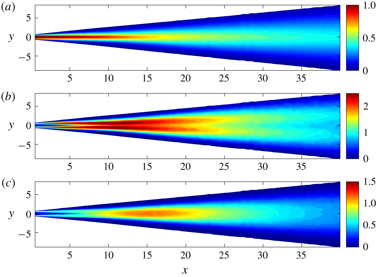
Figure 2. Contour maps of (a)  $U$, (b) $100\overline{uu}$ and (c) $100\overline{vv}$ for the unexcited jet.
In order to quantify some of the trends already observed in figure 2 and verify some theoretical predictions from § 3, figure 3(a) shows characteristic integral properties of the jet for the unforced case. Two methods can be used to obtain these: a direct integration of the measured values at the discrete measured points or, alternatively, by fitting the velocity and normal stress profiles with appropriate laws and then mathematically integrate them. The latter method should in general be preferred as it allows one to decrease the integration error around the jet edges. As visible from the figure, the jet thickness,  $\unicode[STIX]{x1D6FF}$, increases gradually near the channel exit, and for $x>10$, it increases linearly. From the fitted line, a virtual streamwise origin at $x_{0}=3.54$ is found and the spreading rate can be estimated as $\unicode[STIX]{x1D6FD}=0.138$, corresponding to a spreading rate based on $\unicode[STIX]{x1D6FF}_{1/2}$ equal to 0.121. This value is slightly higher than other experiments referred to in § 2.1 and may be due to the evaluation procedure, for the directly integrated data the width is smaller, due to the missing contribution of the tails of the measured velocity profile. In our further evaluation of the measurements we will use the fitted data. The turbulent Reynolds number is $Re_{T}=4/\unicode[STIX]{x1D6FD}\approx 28.6$.

Figure 3. (a) Streamwise evolution of integral jet properties without initial forcing. With (black circles)  $\unicode[STIX]{x1D6FF}$ from the fitting, (black crosses) $\unicode[STIX]{x1D6FF}$ from the direct integration, (blue pluses) measured $U_{c}$, (green triangles) mass flux, $Q$, (red circles) momentum flux, $M_{x}$, (red triangles) mean and turbulent momentum flux, $M_{x}+m_{x}$. The lines are obtained by fitting the experimental data in the last $20d$ demonstrating that $U_{c}\propto 1/\sqrt{x-x_{0}}$, $\unicode[STIX]{x1D6FF}\propto x-x_{0}$ and $M_{x}=4/3U_{c}^{2}\unicode[STIX]{x1D6FF}=\text{const.}$, according to the theory described in § 3. (b) Streamwise distributions of $10u_{rms}$ (red circles), $10v_{rms}$ (black circles) along the jet centreline, (dashed line) $u_{rms}\propto 1/\sqrt{x-x_{0}}$. Both plots have been interpolated to a logarithmic grid to enhance the visibility of the theoretical trends.
The momentum flux is plotted both with ( $M_{x}+m_{x}$) and without ( $M_{x}$) the contribution from the normal stress terms. In both cases it shows a fairly constant value beyond $x=15$. The value from the mean flow and normal Reynolds stresses is 1.01, while the one from the mean flow only is 0.95. It is notable that the contribution of the normal stresses is approximately 5 % of the mean-flow contribution and after the initial transient, the ratio is fairly constant as would be expected if self-similarity holds.
Initially, and up to  $x=5$, the centreline velocity is almost constant, indicating the presence of a core despite the fact that the inlet is a turbulent channel flow. For $x>5$ it starts to decrease as a consequence of the shear layers that have reached the centre of the jet. The volume flow per unit width, $Q$, shows an increase proportional to $(x-x_{0})^{1/2}$ as expected in the self-similar region.
Moving our attention to the velocity covariances, figure 3 $b$ shows the streamwise development of the standard deviation of the measured velocity components along the jet: at 2 diameters downstream of the jet exit the streamwise fluctuation, $u_{c,rms}$, is close to 5 %, typical for a turbulent channel flow at these Reynolds numbers. The value increases further downstream and has a maximum of approximately 14 % around $x=11$ and thereafter decreases and approaches a $-1/2$ slope decay. The distribution of $v_{c,rms}$ is similar to that of $u_{c,rms}$; however, initially it has a lower amplitude, close to 3 %, which is expected for a fully developed channel flow at this Reynolds number (see, for example, Alfredsson & Johansson (Reference Alfredsson and Johansson1984)). Further downstream $v_{c,rms}$ increases and has a maximum around $x=15$.
Profiles of the measured mean velocity components normalised with an artificial centreline velocity,  $U_{c}$, are shown in figure 4. The artificial centreline velocity is obtained by fitting the measured velocity profile to the similarity solution in (3.16) using a least squares method. By normalizing the profiles in this way the development towards similarity is well illustrated. As can be seen, the profiles of the mean streamwise velocity $U$ for $x>15$ are in good agreement with the theoretical profile $U=U_{c}\,\text{sech}^{2}\unicode[STIX]{x1D702}$. The mean transverse velocity profiles, $V$, are also self-similar for $x>15$, although the experimental profiles do not match the theoretical expression (3.19): the centreline gradient is higher while in the outer region the transverse velocity goes to zero but the theory gives a value $|V(\unicode[STIX]{x1D702}\rightarrow \infty )|\approx 0.07U_{c}$, which is not matched. This latter discrepancy is probably due to the difficulty in measuring a small velocity component as well as limitation of large flow angles. As mentioned in § 6 the calibration range with respect to the velocity was $0.5{-}25~\text{m}~\text{s}^{-1}$. For $x=15$ this limits accurate velocity measurements to $|\unicode[STIX]{x1D702}|<1.5$ and for larger $x$ even smaller values of $|\unicode[STIX]{x1D702}|$. One should also note that, beyond $|\unicode[STIX]{x1D702}|>2$, the mean flow angle, according to the theoretical profiles, is larger than that for the maximum angle ( $\pm 36^{\circ }$) for which the calibration was done and is therefore unreliable. One should also be aware that instantaneously the angle may be larger than the calibration bounds even for $|\unicode[STIX]{x1D702}|<2$.

Figure 4. Profiles of the mean streamwise (a) and transverse (b) velocities. Profiles for  $x<15$ are coloured in red, whereas those for $x>15$ are coloured in green. Black lines show the theoretical profiles.


In figure 5 the profiles of the root mean square (r.m.s.) of the streamwise and transverse velocity components as well as the Reynolds shear stress term are plotted, using the same colour coding as for the mean profiles. For  $u_{rms}$ and $v_{rms}$ one can observe that the data show self-similarity somewhat further downstream than for the mean profiles. However, the $\overline{uv}$ distributions seem to show self-similarity starting already for $x=15$, which may be expected since $\overline{uv}$ is directly related to the mean velocity profile. The comparison with the theoretical expression (3.20) shows qualitative agreement but deviates from the similarity solution in its magnitude. However, the measured maximum value of $|\overline{uv}|$ is in good agreement with the results of Gordeyev & Thomas (Reference Gordeyev and Thomas2000) and Cafiero & Vassilicos (Reference Cafiero and Vassilicos2019). Possible explanations for the difference in $|\overline{uv}|$ distributions between the model and the experiments may be the assumption of a constant eddy viscosity across the jet and/or the assumption that the normal stresses in (3.5) can be neglected.
The  $u_{rms}$ distribution has maxima on each side of the centreline close to the position for the maxima of $|\overline{uv}|$ and $|\text{d}U/\text{d}y|$; i.e. the position where the highest production of turbulence occurs. The correlation $\overline{uv}/u_{rms}v_{rms}$ is also plotted showing a rather wide region where the correlation coefficient is approximately $\pm 0.4$, a value that is also commonly measured in the logarithmic region of wall-bounded flows (Alfredsson & Johansson Reference Alfredsson and Johansson1984).
7.2 Excited velocity field
After having characterised the mean and the covariances of the unexcited jet, we now study the response of the jet to acoustic excitation. Figure 6 $a$ shows the streamwise development of basic flow statistics along the jet centreline for three different forcing amplitudes of a periodic forcing with a frequency of $f=100~\text{Hz}$. As can be seen, the highest forcing amplitude gives a significant contribution to $v_{rms}$.
The three curves showing the development of the periodic forcing,  $\widetilde{v}_{rms}$ are directly obtained from the standard deviation of the phase-averaged signal and are shown in figure 6(b) together with $v_{rms}$ (same data as in figure 6a) for the sake of comparison. The ratios between the initial forcing amplitudes (1:3.2:10) can be directly observed in the figure in the region $8<x<20$, indicating a linear behaviour of the forced periodic component. It can also be noted in figure 6(a) that, in the present range of the initial forcing intensity $v_{0}$, the mean centreline velocity $U_{c}$ does not change significantly with $v_{0}$; i.e. the wave excitation has a small influence on the mean flow.

Figure 6. (a) Streamwise distributions of  $U_{c}$ (blue), $10u_{rms}$ (red), $10v_{rms}$ (black) along the jet centreline for three different initial forcing amplitudes with $f=100~\text{Hz}$. (b) $v_{rms}$ (open symbols) and $\widetilde{v}_{rms}$ (filled symbols). The three different initial forcing amplitudes are denoted by: ○ $v_{0}=2.2\times 10^{-5}$, ▵ $v_{0}=6.9\times 10^{-5}$, ▫ $v_{0}=2.2\times 10^{-4}$. The arrow in (b) indicates the increasing forcing amplitude, as a visual aid. Not all data points are shown since it would lead to overcrowding of the figure.

Figure 7. Contour maps of (a)  $100\tilde{u} _{rms}^{2}$ and (b) $100\tilde{v}_{rms}^{2}$ for the excited jet at $f=50~\text{Hz}$.
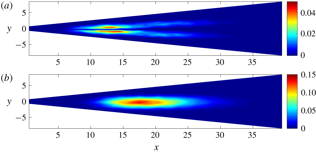
Figure 8. Contour maps of (a)  $100\tilde{u} _{rms}^{2}$ and (b) $100\tilde{v}_{rms}^{2}$ for the excited jet at $f=100~\text{Hz}$.
Figures 7 and 8 illustrate the spatial development of the variance of the periodic velocity component for two different frequencies at  $v_{0}=2.2\times 10^{-5}$. Neither $\tilde{u}$ nor $\tilde{v}$ have their peak immediately at the exit where the excitation source is located, but rather downstream of it with a double-peak distribution for $\tilde{u}$, while $\tilde{v}$ has one peak further downstream. It is interesting to compare figures 7 and 8 with figure 2 since both variance distributions have qualitative resemblances (especially the streamwise component), but the unforced transverse-velocity variance peaks earlier than the periodic one. The difference in frequency of a factor of 2 implies a significant shift in space of the educed structure. If one considers the functional dependence of the mode in the far field of the jet $\tilde{u} =g_{1}(U_{c},\unicode[STIX]{x1D6FF},x-x_{0},y;f,v_{0})$ (all variables are dimensional in this expression and until equation (7.2)), considers that $\unicode[STIX]{x1D6FF}\propto x-x_{0}$, replaces $U_{c}$ with $M_{\infty }$ (the momentum flux is a constant in the far field), and uses the Buckingham theorem, one gets
 $$\begin{eqnarray}\widetilde{u}=U_{s}g_{2}\left(\frac{x-x_{0}}{L_{s}},\frac{y}{L_{s}};\frac{v_{0}}{U_{s}}\right)\quad \text{with }L_{s}=\left(\frac{M_{\infty }}{f^{2}}\right)^{1/3}\text{ and }U_{s}=(M_{\infty }f)^{1/3}.\end{eqnarray}$$
 Assuming now that the educed structure scales linearly with the perturbation amplitude,  $v_{0}$, one obtains the formula
 $$\begin{eqnarray}\frac{\widetilde{u}}{v_{0}}=g\left(x^{\ast }=\frac{x-x_{0}}{L_{s}},y^{\ast }=\frac{y}{L_{s}}\right).\end{eqnarray}$$
 Equation (7.2) is a result of the Buckingham theorem but it is not the only possible result of it. For instance, by using  $U_{c}$ and $\unicode[STIX]{x1D6FF}$ as scaling quantities, one would have obtained $\tilde{u} /v_{0}=h(\unicode[STIX]{x1D702};x^{\ast })$. Equation (7.2) shows anyhow the strong connection between the mode shape and the frequency and provides a simple scaling relationship to universally describe modes obtained at different frequencies, as demonstrated later on in § 7.3
Examples of velocity spectra are shown in figure 9, both without and with excitation. The spectra are taken at  $x=16$, $y=0.117$ and, for those with excitation, the frequency was $f=165~\text{Hz}$. It is noticeable that the spectra without the excitation have no specific peak even close to the exit, suggesting that the dominant structure in the natural jet case is not a single mode such as the flapping phenomenon observed in a laminar jet. The acoustic forcing is able to excite only one frequency/mode without altering significantly the remaining part of the frequency spectrum. This is true as long as the forcing amplitude is sufficiently small and the emergence of the superharmonic (a footprint of nonlinear interactions) is visible only for the highest excitation amplitude.

Figure 9. Power spectra distributions for the streamwise (a–c) and transverse velocity component (d–f) for three excitation amplitudes: ( $a,d$) $v_{0}=3.9\times 10^{-5}$, ( $b,e$) $v_{0}=1.2\times 10^{-4}$ and ( $c,f$) $v_{0}=3.9\times 10^{-4}$ all in red, while the blue lines indicate the unexcited spectra. The spectra are evaluated at $x=16$, $y=0.117$ ( $\unicode[STIX]{x1D702}=0.07$), $f=165~\text{Hz}$. Black lines show the power law $f^{-5/3}$.

Figure 10. Signals of (a)  $\langle u\rangle /v_{0}=\widetilde{u}/v_{0}$, (b) $\langle v\rangle /v_{0}=\widetilde{v}/v_{0}$, (c) $\langle \widehat{v}^{2}\rangle /(v_{0}U_{0})$ and (d) $\langle \widehat{v}^{3}\rangle /(v_{0}U_{0}^{2})$ at $x=19.5$ and $\unicode[STIX]{x1D702}=1$ for $f=50~\text{Hz}$ and five different excitation amplitudes. With (blue) $v_{0}=6.9\times 10^{-6}$, (red) $v_{0}=1.2\times 10^{-5}$, (black) $v_{0}=2.2\times 10^{-5}$, (magenta) $v_{0}=3.9\times 10^{-5}$, (green) $v_{0}=6.9\times 10^{-5}$.
The time series of the periodic components are shown in figure 10 together with the phase average of the second- and third-order moments of the random transverse velocity for different excitation amplitudes. While the periodic component scales linearly with  $v_{0}$, it is remarkable that also the phase averages of moments of the random component scale linearly. Only the weakest excitation level (indicated with the blue line) shows some ripples, but otherwise a very good collapse of the periodic motions is observed. Such an agreement is present in both the measured velocity components and for higher moments: figure 11 shows for instance the comparison of r.m.s. of the covariances $\langle \widehat{u}_{i}\widehat{u}_{j}\rangle$ while figure 12 shows the third-order correlations. They all have an excellent collapse, demonstrating that the phase averages scale linearly with the perturbation amplitudes regardless of the order. In order to remove frequency components not related to the forcing one, the phase averages were filtered before performing the r.m.s. by means of the Fourier transform and taking the amplitude and phase associated with the forcing.

Figure 11. Distributions of (a)  $\langle \widehat{u}\widehat{u}\rangle _{F,rms}/(v_{0}U_{0})$, (b) $\langle \widehat{v}\widehat{v}\rangle _{F,rms}/(v_{0}U_{0})$, (c) $\langle \widehat{u}\widehat{v}\rangle _{F,rms}/(v_{0}U_{0})$ at $\unicode[STIX]{x1D702}=1$ filtered around the forcing frequency ( $f=50~\text{Hz}$). The colour scheme is the same as the one used in figure 10.

Figure 12. Streamwise distributions of the r.m.s. of the filtered phase-averaged third-order correlations at  $\unicode[STIX]{x1D702}=1$ and $f=50~\text{Hz}$. The colour scheme is the same as the one used in figure 10.
The phase-averaged time series show some nonlinear effects only for the forcing with the highest amplitude. This is further illustrated in figure 13 where the phase average of several moments of the random component are shown. All are normalised with the average performed at  $v_{0,ref}=2.2\times 10^{-5}$ showing that all moments of the random component scale linearly with $v_{0}$ if the forcing amplitude is not excessively high.

Figure 13. Proportionality of  $\langle u\rangle$, $\langle v\rangle$ and $\langle \hat{u} ^{n}\hat{v}^{m}\rangle$ against $v_{0}$. All moments are evaluated at $\unicode[STIX]{x1D702}=1$ and averaged in $14.5\leqslant x\leqslant 34.5$; $2\leqslant n+m\leqslant 5$; $v_{0,ref}=2.2\times 10^{-5}$.
The comparison of the time average of the product of the periodic component (reported in figure 14) shows that the contribution of these structures to the mean flow transport scales well with the perturbation amplitude,  $v_{0}$. This linear behaviour of the phase averages of the higher-order moments of the random components demonstrates that all terms in (4.6) are linear, except the nonlinear term of the periodic component, but that term is negligible for weak forcing. Furthermore, it is inferred that (4.8) with the triple terms, and even higher-order equations, can be treated as linear equations in the weak forcing case.

Figure 14. Distributions of filtered (a)  $\overline{\widetilde{u}_{F}\,\widetilde{u}_{F}}/v_{0}^{2}$, (b) $\overline{\widetilde{v}_{F}\,\widetilde{v}_{F}}/v_{0}^{2}$, (c) $\overline{\widetilde{u}_{F}\,\widetilde{v}_{F}}/v_{0}^{2}$ at $\unicode[STIX]{x1D702}=1$. Same conditions as in figure 10.
7.3 Linear stability results
In the stability analysis the sinuous mode was investigated and the considered domain was bounded between  $y_{min}=0$ and $y_{max}=50$. The boundary conditions on the axis ( $y=0$) are $u=p=\unicode[STIX]{x2202}v/\unicode[STIX]{x2202}y=0$, while at $y_{max}$ the conditions are $u=v=p=0$. The eigenvalue problem (5.9) was solved at every streamwise station by means of a collocation method with 180 Chebyshev polynomials. The 180 collocation points followed a Gauss–Lobatto distribution mapped exponentially in physical space. The base flow assumed for the stability analysis was the one given by (3.16) and (3.19) assuming a linear growth and $\unicode[STIX]{x1D6FD}=0.138$, based on the experimental results. The eddy viscosity was assumed to be constant and equal to the one determined in the theoretical analysis (see (3.14)).

Figure 15. Contour maps of  $\widetilde{u}$ at $v_{0}=2.2\times 10^{-5}$: (a) $f=50~\text{Hz}$, (b) $f=100~\text{Hz}$, (c) weakly divergent linear theory. The fields are scaled by the transverse velocity perturbation at $x^{\ast }=2$.

Figure 16. Contour maps of  $\tilde{v}$ at $v_{0}=2.2\times 10^{-5}$: (a) $f=50~\text{Hz}$, (b) $f=100~\text{Hz}$, (c) weakly divergent linear theory. The fields are scaled by the transverse velocity perturbation at $x^{\ast }=2$.
The linear stability calculations were first done in a parallel-flow framework and then complemented with the weakly divergent correction providing the possibility to compare different streamwise stations and get the spatial mode shape. Figures 15 and 16 report a comparison of the experimentally measured mode and the one from the weakly divergent linear stability analysis. The mode in the experiment is obtained from the phase average of the flow field filtered at the excitation frequency, while the stability result is obtained by multiplying the eigenfunction with the oscillating part in space in (5.5). The obtained modes are then scaled to the value of the transverse velocity component at  $(x^{\ast },y^{\ast })=(2,0)$, as discussed in § 7.2. It is interesting to note that the proposed scaling of the coordinates is able to identify the self-similar shape of the mode regardless of the frequency, and this is valid for both measured velocity components. It is remarkable that the educed mode resembles the mode calculated from linear stability theory in both velocity components, with a slightly larger wavelength for the one obtained from the linear stability analysis. The shape of the initial region is also fairly well characterised by the theory despite the fact that the base flow is not coincident with the theoretical profile used in the calculations. It is also interesting to compare the far-field decay of the mode: thanks to the weakly divergent correction, it is possible to compare the spatial decay of the mode for $x^{\ast }>2$ (namely in the self-similar region), showing again good agreement between the simulations and the experiments.

Figure 17. Root mean square data for  $\unicode[STIX]{x1D702}=0$ of the periodic part of the signal as a function of $x^{\ast }$: $v_{0}=2.2\times 10^{-5}$. With (a) $\widetilde{u}_{rms}/\widetilde{v}_{rms,max}$, (b) $\widetilde{v}_{rms}/\widetilde{v}_{rms,max}$. Data points are for different frequencies: (○) 50 Hz, (▵) 60 Hz, (*) 70 Hz, (▫) 80 Hz. Theoretical stability analysis is shown with: - - - - parallel theory, —— weakly divergent theory (black lines with eddy-viscosity model, red lines without eddy-viscosity model). Note that the stability analysis gives $\widetilde{u}_{rms}=0$ on the centreline since only sinuous modes are considered.

Figure 18. Root mean square data for  $\unicode[STIX]{x1D702}=1$ of the periodic part of the signal as a function of $x^{\ast }$: $v_{0}=2.2\times 10^{-5}$. With (a) $\widetilde{u}_{rms}/\widetilde{v}_{rms,max}$, (b) $\widetilde{v}_{rms}/\widetilde{v}_{rms,max}$. Data points are for different frequencies: (○) 50 Hz, (▵) 60 Hz, (*) 70 Hz, (▫) 80 Hz. Theoretical stability analysis is shown with: - - - - parallel theory, —— weakly divergent theory (black lines with eddy-viscosity model, red lines without eddy-viscosity model).
A more quantitative assessment is shown in figures 17 and 18 where the mode amplitude for both velocity components is plotted along the jet axis ( $\unicode[STIX]{x1D702}=0$) and at $\unicode[STIX]{x1D702}=1$ for several excitation frequencies, providing an estimate of the growth rate of the periodic mode in space. The mode amplitude peaks around $x^{\ast }\approx 1.9$ for the transversal component along the axis and a bit earlier when following the mode along the locus $\unicode[STIX]{x1D702}=1$. No clear trend is visible for the range of frequency considered here, underlining the success of the coordinate scaling. The linear stability results are also reported here from both the parallel theory and the weakly divergent approach. The linear stability mode appears to be slightly wider than the experimental result and this becomes particularly visible in figure 16 and at $\unicode[STIX]{x1D702}=1$ (figure 18) where large gradients of the mode are expected. However, the mode is quantitatively well described by the linear stability analysis. Interestingly, additional stability analyses performed without an eddy-viscosity model are also reported in figures 17 and 18 showing a worse agreement with the present experimental results, supporting the idea that the eddy-viscosity model is beneficial in increasing the accuracy of the model.
8 Discussion and conclusions
In the present work a planar jet exiting from a fully developed turbulent channel flow has been acoustically excited in order to be able to identify coherent structures embedded in uncorrelated random turbulence. This is done through measurements of the streamwise and lateral velocity components which are phase averaged with respect to the excitation. The mean flow was characterised first, and it was in good agreement with the literature in terms of the streamwise velocity profile and spreading rate (although slightly larger). Discrepancies between the similarity solution of the mean transverse velocity and shear stress were observed; however, our results seem to correspond well with the other recent experiments (Gordeyev & Thomas Reference Gordeyev and Thomas2000; Cafiero & Vassilicos Reference Cafiero and Vassilicos2019). In the similarity analysis the assumption of a constant eddy viscosity is needed and used in order to obtain an analytical solution, but the discrepancy between experiments and theory may indicate that this assumption is not fully valid.
Several excitation frequencies and amplitudes were tested and it was possible to extract the periodic mode through phase averaging even for small excitation amplitudes. The analysis of the filtered Navier–Stokes equations provided the governing equation of the perturbation with several linear terms, a quadratic term (related to the nonlinear interaction of the periodic perturbation with itself) and an unknown term (related to the phase average of the product of the incoherent fluctuations). While the nonlinear term is likely to be negligible in the evolution of the perturbation, the last term of (4.8) is instead scaling linearly with the perturbation amplitude, suggesting that the phase average of the incoherent-turbulence moments follows a linear behaviour.
It is interesting to compare the perturbation fields obtained at different frequencies, which show significant differences if physical coordinates are used. Here a coordinate scaling is proposed based on the excitation frequency, that is able to universally scale the perturbation fields. This observation has been further verified by the linear stability analysis, where the same eigenmode was obtained. Some discrepancies between the theoretical predictions and the experimental results were present in the initial stage of the jet development, probably due to the fact that the stability analysis used a velocity profile from the theory rather than from the measurements, but the agreement in the perturbation decay became very good in the later self-similar stage.
When the acoustic forcing is not too strong the periodic components scale linearly with the forcing amplitude. The successful prediction for the structure and growth of the periodic components by linear theory implies that the linear dynamics of modal perturbations are embedded in the turbulent environment. This is in support of the idea that the large-scale perturbations in the jet could be regarded as an incoherent set of linear modes and suggests that a successful strategy for control of turbulent jets should focus on the linear-mode dynamics.
If the linear behaviour of phase averages of velocities and moments of random components can be observed also in wall-bounded flows (boundary layers and channel flows), then it should be possible to analyse coherent structures, such as streaks and wall-attached eddies, based on the phase-average equations such as (4.6).
Acknowledgements
The experimental set-up was built by T. Yamauschi, whereas S. Tazoe and S. Aruga did the measurements used in the present paper. H. Alfredsson wants to thank the Japan Society for the Promotion of Science for supporting an Invitational Fellowship to Shinshu University.
Declaration of interests
The authors report no conflict of interest.


 Open access