


1 Introduction
Thy dynamics of swimming and flying differ significantly between the observable behaviour in nature and engineering solutions. Flow separation in quasi-steady flows (e.g. on fixed wings and rigid bodies) usually leads to significant losses of propulsive efficiency and control authority, and hence is generally avoided in most engineering applications. In contrast, during a propulsive stroke in nature, animals utilise accelerating and morphing propulsors to actively trigger flow separation, as sketched in figure 1. At the vortex-forming edge (VFE; marked green in figure 1), a shear layer separates from the propulsor. Subsequently, the shear layer rolls up to form a vortical structure. Fluid–structure interaction between the vortex and the propulsor leads to the production of lift and thrust, while maintaining manoeuvrability. Comprehensive overviews of animal locomotion are given by Azuma (Reference Azuma2006), Shyy et al. (Reference Shyy, Lian, Tang, Viieru and Liu2007) and Biewener & Patek (Reference Biewener and Patek2018) to name but a few.

Figure 1. Undulatory modifications of the VFE (depicted in green): (a) leopard frog (sketch abstracted from Johansson & Lauder (Reference Johansson and Lauder2004)); (b) sea lion (sketch abstracted from Sawyer, Turner & Kaas (Reference Sawyer, Turner and Kaas2016)); and (c) humpback whale (sketch abstracted from Fish & Lauder (Reference Fish and Lauder2006)).
According to Pitt Ford & Babinsky (Reference Pitt Ford and Babinsky2013), the importance of the unsteady vortex to lift and thrust is defined by its circulation, as the vortex contains most of the circulation bound to the propulsor. However, when the vortex sheds, the associated forces are reduced significantly. As a consequence, the influencing factors on the circulation of the vortex wake and its stability have been widely addressed in recent studies. Examples include the role of rotational accelerations (see e.g. Lentink & Dickinson Reference Lentink and Dickinson2009), propulsor flexibility (see e.g. Vanella et al. Reference Vanella, Fitzgerald, Preidikman, Balaras and Balachandran2009), spanwise curvature (see e.g. Taira & Colonius (Reference Taira and Colonius2009), Hartloper & Rival (Reference Hartloper and Rival2013)), swept wings (see e.g. Wong & Rival (Reference Wong and Rival2015)) and the interaction of the vortex with secondary boundary layers (Eslam Panah, Akkala & Buchholz Reference Eslam Panah, Akkala and Buchholz2015; Akkala & Buchholz Reference Akkala and Buchholz2017).
This study aims to extend the above studies towards a characterisation of the effects of small-scale structures in unsteady flows, and their relevance towards the resulting vortex dynamics. In particular, we strive to draw insight into the influence of turbulence and associated coherent flow structures of different length scales on the vortex formation process. Inspired by undulated modifications on the VFE of multiple propulsors in nature (see figure 1), this problem is tackled with a combined study of vortex formation over a wide range of  $Re$ superimposed with various VFE modifications. While an increase of $Re$ is known to extend the range of turbulent substructures towards additional smaller vortices, VFE modifications allow for the introduction of disturbances with distinct wavelengths $\unicode[STIX]{x1D706}$, which are predetermined by the propulsor itself.
1.1 Background on the  $Re$ scaling of vortex formation and shear layers

Various swimmers and flyers across diverse species utilise separated flows during their locomotion. Inspired by this evolutionary convergence, prior studies applied dimensional analysis to extract commonalities in shape and kinematics for a large variety of propulsors. These common shapes and kinematics developed independently and from different lineages. For instance, Chin & Lentink (Reference Chin and Lentink2016), among others, characterised leading-edge vortices (LEVs) through dimensionless quantities such as Rossby number ( $Ro$), Strouhal number ( $St$) and Reynolds number ( $Re$). In particular, $Ro$, i.e. the relation between centripetal and Coriolis forcing due to rotational accelerations of the wing, was emphasised as crucial for long-term LEV stability. Furthermore, Lentink & Dickinson (Reference Lentink and Dickinson2009) revealed a limit to values of $Ro<4$ in nature across diverse species.
Plunging and pitching kinematics are characterised by the reduced frequency ( $k$) and the Strouhal number. Again, a narrow band of values $0.2\leqslant St\leqslant 0.4$ tends to deliver maximum efficiency and can be found for both flyers (Taylor, Nudds & Thomas Reference Taylor, Nudds and Thomas2003) and swimmers (Triantafyllou, Triantafyllou & Gopalkrishnan Reference Triantafyllou, Triantafyllou and Gopalkrishnan1991). In contrast, propulsors ranging from fruit flies to large cetaceans use vortical structures for efficient propagation, which according to Gazzola, Argentina & Mahadevan (Reference Gazzola, Argentina and Mahadevan2014) corresponds to a rather large Reynolds-number range of $10^{2}\leqslant Re\leqslant 10^{8}$. The convergence over a wide range of $Re$ found in nature suggests a small influence of the small-scale structures in the flow onto the vortex formation process and the associated loadings. The above result that small scales do not influence vortex formation is unexpected since various studies indicate a $Re$-dependent formation of separated shear layers. The review on quasi-steady shear layers by Ho & Huerre (Reference Ho and Huerre1984) indicates an essentially inviscid mechanism behind the dominant instability mechanism in free shear layers: Kelvin–Helmholtz instability (KHI). However, small-scale mixing and entrainment are still dominated by viscous effects, as discussed by Wolf et al. (Reference Wolf, Holzner, Lüthi, Krug, Kinzelbach and Tsinober2013) and Chauhan, Philip & Marusic (Reference Chauhan, Philip and Marusic2014). Furthermore, Rosi & Rival (Reference Rosi and Rival2018) extended this observation for accelerating shear layers and showed that for acceleration the spacing of KHIs varies strongly with $Re$.
$Re$.
By conducting experiments over a wide range of  $Re$, the present study attempts to address the paradox that, on the one hand, the $Re$ influence based on dimensional analysis seems to be small, yet, on the other hand, the entrainment in free shear layers is influenced by the small structures and thus $Re$. Particular focus lies on the interaction of the $Re$ scaling with the aforementioned VFE modifications.
1.2 Background on vortex-forming edge modification
For quasi-steady flows, applications of passive flow control by means of geometrical modifications are well established, as already outlined by Carmichael (Reference Carmichael1981). For instance, Lissaman (Reference Lissaman1983) demonstrated significant delay of flow separation on stalling airfoils by means of tripping strips, fixed at the respective leading edges. Similarly, vortex generators and bio-inspired serrations have been applied for airfoil flow control by Lin (Reference Lin2002) and Ito (Reference Ito2009), respectively. Furthermore, lobe mixers have been proven by McCormick & Bennett (Reference McCormick and Bennett1994) to reduce the noise through mixing in the wake of jet engines. These examples underline the importance of the nonlinear impact of convective effects, where the introduction of small-scale structures leads to a significant change in behaviour of the global system.
In the category of separated flows, Usherwood & Ellington (Reference Usherwood and Ellington2002), Rival et al. (Reference Rival, Kriegseis, Schaub, Widmann and Tropea2014) and Leknys et al. (Reference Leknys, Arjomandi, Kelso and Birzer2018) investigated the influence of mild VFE modifications for accelerating propulsors. Motivated by the reports of Hertel (Reference Hertel1966) on the dragonfly-wing leading edge, Usherwood & Ellington (Reference Usherwood and Ellington2002) imprinted a spanwise saw-like structure on the VFE under consideration. This study – most likely due to the choice of a single wavelength – did not reveal notable influences of VFE modifications on the flow and the measured forces. Rival et al. (Reference Rival, Kriegseis, Schaub, Widmann and Tropea2014) and Leknys et al. (Reference Leknys, Arjomandi, Kelso and Birzer2018) focused on small changes of the leading-edge curvature and reported small yet measurable delays on vortex formation.
The high impact of nonlinear effects onto quasi-steady flows and the already measurable influence of VFE modifications in the case of small VFE modifications suggest that there is merit in further investigation of a wider range of introduced disturbances in separated flows. This is supported by the observation of significant VFE modifications on propulsors in nature. The list of examples – even though from strongly differing lineages – includes webbed frog feet (e.g. Johansson & Lauder Reference Johansson and Lauder2004), the hind limbs of sea lions (e.g. Sawyer et al. Reference Sawyer, Turner and Kaas2016) and the tubercles on the flippers of humpback whales (e.g. Fish & Lauder Reference Fish and Lauder2006); see also figure 1. Note that each of those VFE modifications is of distinct wavelength  $\unicode[STIX]{x1D706}$, all significantly smaller than the length scale $L$ of the propulsor itself.
1.3 Objectives and procedure
The combined effects of VFE modification and  $Re$ scaling are investigated on the reference case of an impulsively accelerated, rigid circular plate of diameter $D$. This canonical flow for vortex formation was recently characterised by Fernando & Rival (Reference Fernando and Rival2016b) and combines several features, qualifying it as a suitable base case for this study. First, the lack of leading-edge sweep, no rotational accelerations of the propulsor and the absence of wing-tip or wing-body effects minimises three-dimensional effects during vortex formation. Thus, the influence of small scales in the flow can be observed without being superimposed by complex, global and three-dimensional flow features. Second, Fernando & Rival (Reference Fernando and Rival2016a) showed that, in contrast to non-circular propulsors, the circular case produces a stable vortex, which only pinches off after multiple diameters $D$ travelled. The stable vortex allows a longer observation time and provides the possibility to investigate the effects of VFE modifications onto vortex stability. The bio-inspired VFE modifications are abstracted from the undulatory examples mentioned in § 1.1 and modelled by adding a cosine function of different wavelengths $\unicode[STIX]{x1D706}$ with amplitude $a=\unicode[STIX]{x1D706}/4$ onto the circular edge geometry; see § 2.1 for more parameter details.

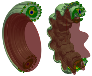
Figure 2. Summary sketches of possible flow topologies around various plate geometries; (a–c) the shear layer directly after the onset of acceleration for different plate geometries; and (d–i) different possible vortex formation topologies for varying  $Re$ and plate geometries.
Early on during the onset of vortex formation, a thin layer of vorticity is produced along the VFE on the varying plates, as indicated in figure 2(a–c). While the frontal area remains constant for all plates, the effective perimeters vary due to the superimposed waves. Therefore, it is expected that the magnitude and orientation of vorticity generated on the edge should vary between the different geometries. During the subsequent vortex formation, the shear layer detaches, rolls up and forms a vortex. For the circular plate, the vortex evolution is well known (see figure 2d). The KHIs appear during the plate’s acceleration and are continuously produced during the whole vortex formation process, as has been shown by Wong et al. (Reference Wong, Rosi, Rouhi and Rival2017) and Rosi & Rival (Reference Rosi and Rival2017). A high-vorticity core remains stable until azimuthal instabilities appear and destabilise the system. The wavelength of the azimuthal instabilities and their onset in a circular vortex ring depend on  $Re$, which has been shown by Maxworthy (Reference Maxworthy1977) for vortices produced by a classical piston–cylinder vortex generator. Fernando & Rival (Reference Fernando and Rival2016b) confirmed the existence of the azimuthal instability for vortex rings in the wake of an accelerated circular plate.
For the geometries with VFE modifications, however, the formation of the vortex wake is yet unknown. Various wakes seem possible, all of which are outlined in figure 2. It is hypothesised that the relation
 $$\begin{eqnarray}B=\unicode[STIX]{x1D706}/2\unicode[STIX]{x1D6FF}\end{eqnarray}$$
 of the undulatory VFE modification height  $\unicode[STIX]{x1D706}/2$ to shear-layer thickness $\unicode[STIX]{x1D6FF}$ is a crucial relative quantity. Therefore, the flow around the plates is colour-coded accordingly in figure 2, where red indicates flow around a smooth circular plate, and green corresponds to VFE wavelengths in the order of magnitude of the shear-layer thickness or smaller ( $B\leqslant 1$). The flow around plates with VFE modifications with significantly larger wavelengths is visualised in blue ( $B\gg 1$). Three flow topologies seem possible for small $\unicode[STIX]{x1D706}$ ( $B\leqslant 1$). As a trivial solution, the effects of the VFE modifications might be irrelevant or directly damped out such that the vortex formation would then appear similar as for the unmodified circular plate (see figure 2e). The disturbances introduced by the undulated VFE could also promote transition to a turbulent shear layer, where the presence of turbulent small-scale structures directly corrupts the forming KHIs (see figure 2g). Recent reports by Buchner, Honnery & Soria (Reference Buchner, Honnery and Soria2017) suggest that a change of the dominant instability mechanism towards centrifugal instabilities (CIs) is also possible. Small-scale VFE modifications could favour the formation of CIs, as indicated in figure 2(h). The shear layer of larger undulatory VFE modifications $\unicode[STIX]{x1D706}$ ( $B\gg 1$) might reorient towards a circle and roll up as discussed for the smaller perturbations (similar to figure 2e). In contrast, a complete disruption of the vortex formation process and an expedited transition to the fully separated and turbulent state also seems possible (see figure 2f). However, a mixture between these above cases is most likely: a destabilised shear layer that rolls up to a complex turbulent flow with a diffuse vortex core, as sketched in figure 2(i).
As a consequence of the above-outlined variety of possible flow conditions and hypotheses, the objective of the present work centres around which VFE modifications influence the unsteady vortex wake behind accelerating propulsors. A systematic variation of  $\unicode[STIX]{x1D706}$ across a wide range of $Re$ is performed by means of time-resolved particle image velocimetry (PIV) and force measurements in an optical towing tank. The resulting data serve as a basis to study the instability mechanisms as they occur with varying wavelength $\unicode[STIX]{x1D706}$ and/or $Re$. In particular, the footprint of the VFE modifications in the vortex formation is evaluated with respect to the resulting loading on the propulsor and the stability of the vortex wake itself.
2 Methods
2.1 Kinematics and parameter space
The kinematics and the  $Re$ space are chosen to match the previous study by Fernando & Rival (Reference Fernando and Rival2016b). The plates of mean diameter $D$ are impulsively accelerated perpendicular to their orientation to a terminal velocity of $U_{\infty }$ within a distance of $s^{\ast }=s/D=0.5$, where $s$ is the physical distance travelled. Two terminal velocities $U_{\infty }$ are compared, which correspond to $Re=U_{\infty }D/\unicode[STIX]{x1D708}=50\,000$ and $Re=350\,000$ based on constant values for plate diameter $D$ and kinematic viscosity of water $\unicode[STIX]{x1D708}$.

Figure 3. (a) Sketch of the chosen vortex-edge modification; wavelength  $\unicode[STIX]{x1D706}$, undulatory disturbance amplitude $a$ and mean plate diameter $D$. (b) Geometries with number of undulations $n_{p}=\infty$, $n_{p}=12$, $n_{p}=50$ and $n_{p}=200$.
Three plates with undulatory VFE modifications of varying wavelengths  $\unicode[STIX]{x1D706}$ are compared to a smooth circular plate ( $n_{p}=\infty$). The mean perimeter $\unicode[STIX]{x03C0}D$ is divided into $n_{p}$ waves of length $\unicode[STIX]{x1D706}=\unicode[STIX]{x03C0}D/n_{p}$. To avoid the introduction of additional (and confusing) length scales into the system, the wavelength $\unicode[STIX]{x1D706}$ and amplitude $a$ of the introduced undulations are held constant at a ratio of $a/\unicode[STIX]{x1D706}=1/4$. Consequently, the radius of the modified plates is defined as
 $$\begin{eqnarray}R(\unicode[STIX]{x1D711})=D/2+\unicode[STIX]{x1D706}/4\cos (n_{p}\unicode[STIX]{x1D711}),\end{eqnarray}$$
 which is indicated in figure 3(a). The frontal surface area  $A$ of all plates is held constant, which is achieved by iteratively adjusting $D$. Note that the addition of the cosine function in combination with a constant frontal area $A$ implies different perimeters $P$ for plates of different wavenumbers $k_{p}=1/\unicode[STIX]{x1D706}=n_{p}/\unicode[STIX]{x03C0}D$. In particular, the influence of the number of undulations, $n_{p}=12$, $n_{p}=50$ and $n_{p}=200$, is tested. Additionally, the experiments for a circular plate ( $n_{p}=\infty$) from Fernando & Rival (Reference Fernando and Rival2016b) are repeated for reference and comparison. All plate geometries considered are shown in figure 3(b); the geometrical details are also listed in table 1. The plate with $n_{p}=50$ leads to a length scale $2a$ similar to the spacing of KHIs and the shear-layer thickness $\unicode[STIX]{x1D6FF}$ ( $B\approx 1$). Accordingly, undulatory VFE modifications with larger or smaller wavelengths ( $n_{p}=200$ and $n_{p}=12$) introduce structures that are smaller ( $B<1$) or larger ( $B>1$) than the shear-layer thickness, respectively.

Figure 4. Optical towing tank (a) and PIV set-up (b). The light sheet enters the tank from the bottom window; multiple high-speed cameras (A, B and C) capture the accelerating plate in a lab-fixed frame of reference.
Table 1. Parameters describing the various plate geometries tested here.

2.2 Experimental set-up
The experiments were conducted in the 15 m long optical towing tank facility at Queen’s University, as shown in figure 4(a). The cross-section spans  $1~\text{m}\times 1~\text{m}$ and is optically accessible from three sides. An overhead traverse is used to tow models, where an additional non-transparent semi-enclosed ceiling minimises free-surface effects. In the present study, the four plates considered were mounted onto a cylindrical sting with a diameter of $0.08D$ and length $2D$, which was further connected to the traverse by a symmetric profile of thickness $0.08D$. A six-component, submersible ATI Nano force transducer was applied between the sting and the plates to record force data at 1000 Hz with a static resolution of $0.125~\text{N}$ (see figure 4b). Every parameter combination was repeated 20 times for $s^{\ast }\leqslant 33$ and the data were ensemble-averaged accordingly.
Complementary to the force measurements, the flow fields in the wake of all plates were captured by means of time-resolved planar PIV, as shown in figure 4(b). A 2 mm thick light sheet was created through a  $40~\text{mJ}~\text{pulse}^{-1}$ Photonics high-speed laser, and then introduced into the tank through the bottom window. The light sheet was centred parallel to the sidewalls in the tank and was tilted towards the towing direction to avoid shadows in the wake.

Figure 5. Overlapping FOVs and campaigns of the conducted PIV experiments (plate motion from right to left).
Table 2. Overview of the conducted experiments; roman numerals I–VII correspond to different FOVs of the PIV set-up; cf. also figure 5.

Three multi-camera PIV campaigns were performed in a lab-fixed frame of reference, as illustrated in figure 5 and listed in table 2. Raw images were recorded at 200 frames per second (f.p.s.) for  $Re=50\,000$ and 1400 f.p.s. for $Re=350\,000$. Note that for plate $12$ ( $n_{p}=12$) the PIV measurements were performed twice per $Re$, where the light sheet was either aligned with the maximum or with the minimum of the plate radius ( $r=169.3~\text{mm}$, $r=129.3~\text{mm}$). These two measurements are from here on referred to as 12top and 12bot. Similar to the force measurements, 20 runs of PIV data collection were performed for each set of parameters throughout all campaigns.
Three cameras were used during the first measurement campaign to cover a combined field of view (FOV) of  $s^{\ast }=0{-}2.3$ on the bottom half of the plate (see figure 5). The early acceleration stage was captured in a small FOV (I in figure 5) of $0.7D\times 0.7D$ with a Photron Fastcam Mini WX100 ( $2048\times 2048$ pixels, camera A) to ensure sufficient spatial resolution near the VFE. Two additional Photron SA4 cameras ( $1024\times 1024$ pixels, cameras B and C) captured the further evolution of the vortex, where larger FOVs of $0.85D\times 0.85D$ (II and III in figure 5) were chosen to account for the vortex growth. All cameras were equipped with AF-S Micro-Nikkor 60 mm 1:2.8G ED lenses, which resulted in a resolution of $9.8~\text{pixel}~\text{mm}^{-1}$ (FOV I) and $4~\text{pixel}~\text{mm}^{-1}$ (FOVs II and III).
Owing to frame rate limitations, camera A (Mini WX100) was only used for the lower- $Re$ cases. The evaluation of the first campaign (i.e. the force measurements), however, provided evidence to investigate later vortex formation stages – particularly for the high- $Re$ case. This insight will be elaborated in more detail in § 3. Therefore, two additional PIV campaigns were performed for the circular and the $n_{p}=12$ plate and the higher $Re$ ( $Re=350\,000$). The two Photron SA4 cameras (cameras B and C) were readjusted to allow for an even larger FOV of $1.0D\times 1.0D$ and were used to measure the vortex evolution from $s^{\ast }=2.3{-}4.2$ (campaign 2 – FOVs IV and V) and $s^{\ast }=4.2{-}6.1$ (campaign 3 – FOVs VI and VII). The frame rates were kept identical to campaign 1, but, owing to the larger FOV, the resolution decreased to $3.4~\text{pixel}~\text{mm}^{-1}$.
The raw images were pre-processed in MATLAB in terms of ensemble-based median subtraction, edge detection and plate tracking, and masking of the shadowed area. DaVis 8.4 was used to calibrate and process the data of each camera separately. A multi-grid scheme with a final interrogation area of  $32\times 32$ pixels and 75 % overlap was chosen for FOVs II–VII. FOV I was evaluated with an interrogation area of $48\times 48$ pixels and 75 % overlap. The resulting velocity fields of all 20 runs were ensemble-averaged for each FOV. Finally, all FOVs were merged on a common plate-fixed grid. Note that the interplay of accurate calibration, edge tracking and good reproducibility of the flow even allows stitching of the separate campaigns to a single FOV.
2.3 Analysis methods
To further analyse the ensemble-averaged and merged velocity fields, various post-processing strategies are applied, each of which is outlined in this section and indicated in figure 6.
Hunt, Wray & Moin (Reference Hunt, Wray and Moin1988) introduced the second invariant  $Q$ of the velocity gradient tensor as a robust means to locate vortical structures. Its maximum $Q^{max}$ is frequently applied to localise the core of such structures. More recently, Graftieaux, Michard & Grosjean (Reference Graftieaux, Michard and Grosjean2001) proposed two criteria ( $\unicode[STIX]{x1D6E4}_{1}$ and $\unicode[STIX]{x1D6E4}_{2}$) to identify the core and boundaries of vortical structures, respectively. Huang & Green (Reference Huang and Green2015) showed that $\unicode[STIX]{x1D6E4}_{1}^{max}$ and $Q^{max}$ lead to similar core locations in cases where the reference frame for $\unicode[STIX]{x1D6E4}_{1}$ was chosen appropriately, as indicated in figure 6(a) for a plate-fixed frame of reference. However, the location $r_{c}(t),z_{c}(t)$ of the vortex core is estimated based on the Galilean invariant $Q^{max}$ throughout the present work to avoid any possible uncertainties resulting from reference-frame issues.
The Galilean invariant  $\unicode[STIX]{x1D6E4}_{2}$-criterion is chosen to identify the boundaries of vortical structures for $\unicode[STIX]{x1D6E4}_{2}=2/\unicode[STIX]{x03C0}$. The core locations $r_{c}(t),z_{c}(t)$ are enclosed by one such boundary (see black line in figure 6a), which is referred to as vortex core area $A_{\unicode[STIX]{x1D6E4}_{2}}$. The equivalent diameter $d$ and corresponding circulation $\unicode[STIX]{x1D6E4}_{c}$ of the vortex core are determined by
 $$\begin{eqnarray}d=2\sqrt{\frac{A_{\unicode[STIX]{x1D6E4}_{2}}}{\unicode[STIX]{x03C0}}}\end{eqnarray}$$
and
 $$\begin{eqnarray}\unicode[STIX]{x1D6E4}_{c}=\int _{A_{\unicode[STIX]{x1D6E4}_{2}}}\unicode[STIX]{x1D714}_{\unicode[STIX]{x1D711}}\,\text{d}A,\end{eqnarray}$$
respectively.

Figure 6. Sample processing for case 12top,  $s^{\ast }=3.5$. (a) Overview of applied methods: $(x^{\prime },y^{\prime })$ coordinate system aligned with the shear layer (red); vortex core centres ( $r_{c},z_{c}$) determined with $\unicode[STIX]{x1D6E4}_{1}$ and $Q$; horizontal line through the vortex core (light blue); vortex core boundaries evaluated with $\unicode[STIX]{x1D6E4}_{2}$ (black); control volume for total vortex circulation (orange). (b) Velocity vectors and vorticity contours of the $(x^{\prime },y^{\prime })$ domain (red box). (c) Spatially averaged profiles of velocity $\langle u_{y^{\prime }}\rangle _{y^{\prime }}$ and vorticity $\langle \unicode[STIX]{x1D714}_{\unicode[STIX]{x1D711}^{\prime }}\rangle _{y^{\prime }}$. Black lines in panels (b) and (c) indicate the domain for the calculation of circulation flux $\dot{\unicode[STIX]{x1D6E4}_{sl}}$.
An estimate of total vortex circulation  $\unicode[STIX]{x1D6E4}$ including the shear layer is derived from the integration of vorticity across a large control volume behind the plate, which is highlighted orange in figure 6(a). The lower boundary of the control volume is fixed at $r/D=0.19$ to exclude the secondary vortex from the circulation budget. The secondary vortex occurs during the later stages of the flow and near the centre of the plate; see § 3.
Recent reports on vortex formation evaluated the convective fluxes through a cut perpendicular to the propulsor and directly behind the flow separation to estimate the circulation flux  $\dot{\unicode[STIX]{x1D6E4}_{sl}}$ from the shear layer into the vortex; see for instance Eslam Panah et al. (Reference Eslam Panah, Akkala and Buchholz2015) or Akkala & Buchholz (Reference Akkala and Buchholz2017). The present work attempts to advance beyond this plate-oriented approach to overcome two shortcomings. First, the optical access to the shear layer is blocked in the immediate vicinity of the VFE for 12bot, since the plate is an obstruction in front of the light sheet due to radius changes; see (2.1). The velocity information in this region, therefore, remains unknown. Second, instabilities in the shear layer lead to a strong fluctuation of the circulation flux over time due to KHIs.
Consequently, the flux evaluation is shifted slightly leeward and away from the solid structure, and a spatial average of the shear layer is evaluated to smooth the effects of instabilities. This four-step approach is illustrated in figure 6. First, the average velocity of the shear layer is evaluated in the red dashed area behind the plate to determine the shear-layer orientation. This direction is then aligned with the  $y^{\prime }$-axis of a $(x^{\prime },y^{\prime })$ coordinate system. A close-up of this tilted $(x^{\prime },y^{\prime })$ domain (solid red box) is shown in figure 6(b). Profiles of spatially averaged velocity $\langle u_{y^{\prime }}\rangle _{y^{\prime }}$ and out-of-plane vorticity $\langle \unicode[STIX]{x1D714}_{\unicode[STIX]{x1D711}}\rangle _{y^{\prime }}$ along $y^{\prime }$ are shown in figure 6(c). The origin of $x^{\prime }$ is set to collapse with the maximum of $\langle \unicode[STIX]{x1D714}_{\unicode[STIX]{x1D711}}\rangle _{y^{\prime }}$. The spatial filter along $y^{\prime }$ minimises the influence of remaining PIV uncertainties and small-scale instabilities in the shear layer.
Despite slight shear-layer thickness variations, a band of  $-0.025D<x^{\prime }<0.025D$ was found to be a reasonable and robust domain for the circulation-flux calculation, since $\unicode[STIX]{x1D714}_{\unicode[STIX]{x1D711}}\approx 0$ in the vicinity of the shear layer:
 $$\begin{eqnarray}\dot{\unicode[STIX]{x1D6E4}_{sl}}=\int _{x^{\prime }=-0.025D}^{0.025D}\langle u_{y^{\prime }}\rangle _{y^{\prime }}\langle \unicode[STIX]{x1D714}_{\unicode[STIX]{x1D711}}\rangle _{y^{\prime }}\,\text{d}x^{\prime }.\end{eqnarray}$$
 Note that more accurate strategies to approximate the shear-layer thickness (see e.g. Brown & Roshko Reference Brown and Roshko1974) do not apply for the present data, as only  ${\approx}5{-}6$ velocity vectors are found within the width of the shear layer itself.

Figure 7. Force history  $C_{d}(s^{\ast })$ for all plate geometries and $Re$; the shaded area indicates the scatter through a $2\unicode[STIX]{x1D70E}$ uncertainty margin. Significant force deviations for the $n_{p}=12$ plate are emphasised in the close-up of panel (b).
3 Results
First, the impact of edge undulations and  $Re$ scaling on the overall force histories is evaluated in § 3.1. Complementary to force measurements, velocity and ensemble-averaged vorticity fields provide insight into the underlying flow patterns for varying VFE modifications and $Re$, as addressed in § 3.2.
3.1 Forces
The force histories of each run were temporally filtered with a least-squares estimator as per Savitzky & Golay (Reference Savitzky and Golay1964) and ensemble-averaged across 20 runs. Subsequent normalisation of the force (drag) was performed as follows:
 $$\begin{eqnarray}C_{d}=\frac{2|F_{z}|}{\unicode[STIX]{x1D70C}AU_{\infty }^{2}},\end{eqnarray}$$
 as presented in figure 7. To further check the repeatability of the measurements and uncover significant case-to-case variations, two standard deviations  $(\pm 2\unicode[STIX]{x1D70E})$ are added to the plots. The small uncertainty margins during acceleration, with its associated added-mass peak ( $0.0\leqslant s^{\ast }\leqslant 0.5$), relaxation stage ( $0.5<s^{\ast }<2.5$) and the stable vortex-growth stage ( $2.5\leqslant s^{\ast }\leqslant 5$ for $Re=50\,000$, $2.5\leqslant s^{\ast }\leqslant 9$ for $Re=350\,000$) indicate good repeatability. Once the flow destabilises and detaches from the plate, the run-to-run scatter increases by an order of magnitude, which indicates the sensitivity of this instability-triggered topology change. Finally, beyond $s^{\ast }>20$, the fully separated and turbulent flow collapses to similar terminal values $C_{d}$, which implies that this stage is stable and highly repeatable again.
Interestingly, no significant variations of the drag coefficient are found between the circular reference plate and the small-scale modifications  $n_{p}=50$ and $n_{p}=200$ for both $Re$ – despite considerable changes in the perimeter. Only the force history of the $n_{p}=12$ plate deviates from the circular base case, which still lies within the uncertainty margin for $Re=50\,000$ (see figure 7a). For $Re=350\,000$, in contrast, the $n_{p}=12$ plate generates a significantly higher force during the vortex-growth stage as compared to the reference and small-scale cases. A close-up of this difference is added to figure 7(b) so as to emphasise the 20 % offset in relation to the small uncertainty margin. Note that the abscissa of the inset starts from $s^{\ast }=2.0$, since the forces are significantly higher during the early acceleration ( $s^{\ast }\leqslant 0.5$) and relaxation ( $0.5<s^{\ast }<2.5$). During the acceleration, the forces collapse for identical plate cross-sections $A$.
$A$.
The force deviation for the stable vortex-growth stage implies that the large-amplitude VFE modification of the  $n_{p}=12$ plate significantly influences the vortex formation process. However, the vortex topology remains similar in the wake. Consequently, the wavy shear layer still rolls up into a vortex, which remains attached to the plate for a comparable duration as with the circular reference case. To explore these differences, we now turn to the flow fields.
3.2 Field data
To compare the early vortex formation process ( $1.25\leqslant s^{\ast }\leqslant 2.25$) of the various plate geometries, the vorticity fields for all cases are shown in figures 8 and 9 for $Re=50\,000$ and $Re=350\,000$, respectively. Note that only selected vorticity fields are displayed here for the sake of brevity. The complete temporal evolution ( $s^{\ast }<2.3$) of all cases is provided in a supplementary movie (see Movie1.mp4) available at https://doi.org/10.1017/jfm.2019.908.

Figure 8. Early vortex formation at  $Re=50\,000$: vorticity fields in the range of $1.25\leqslant s^{\ast }\leqslant 2.25$ for all plate geometries. Similar results for no and small-scale VFE modifications ( $n_{p}\in \{\infty ,200,50\}$) – also applies for $Re=350\,000$, cf. figure 9. KHI length scale variation and convection of oppositely signed vorticity from the leeward boundary layer for large-scale VFE modifications ( $n_{p}=12$).

Figure 9. Early vortex formation at  $Re=350\,000$: vorticity fields in the range of $1.25\leqslant s^{\ast }\leqslant 2.25$ for all plate geometries. Similar results for no and small-scale VFE modifications ( $n_{p}\in \{\infty ,200,50\}$). Note that the KHI spacing remains constant for the small-scale VFE modifications ( $n_{p}\in \{\infty ,200,50\}$), but is reduced for $n_{p}=12$ at $Re=350\,000$ compared to $Re=50\,000$, cf. figure 8.
The circular plate (Base,  $n_{p}=\infty$) and the high-wavenumber plates ( $n_{p}=50$ and $n_{p}=200$) reveal similar results in the force measurements for both $Re$ (see figure 7). The corresponding PIV measurements confirm these results, where the similarity of the extracted vorticity fields (see figures 8 and 9) indicates that similar topologies during the early relaxation stage ( $s^{\ast }=1.25$) and during the late relaxation stage ( $s^{\ast }=2.25$) are equivalent for the three geometries ( $n_{p}\in \{\infty ,200,50\}$) and both $Re$. The strong repeatability of the measurements, furthermore, leads to clear visualisations of the dominant KHI. Neither disturbances smaller than the shear-layer thickness $\unicode[STIX]{x1D6FF}$ ( $B<1$, $n_{p}=200$) nor disturbances of the same order of magnitude ( $B\approx 1$, $n_{p}=50$) affect the instability mechanism or lead to significant corruption of the KHI. Also, the influence of $Re$ onto the instabilities is small, since the same spatial offsets of consecutive KHI structures are found in the shear layer for both $Re$; compare figures 8(a)–(i) and 9(a)–(i). It is important to mention at this point that this finding does not hold for the earlier stage of plate acceleration ( $s^{\ast }<0.5$), as reported by Rosi & Rival (Reference Rosi and Rival2017).
The similarity between the circular case and the small-scale VFE modifications ( $n_{p}\in \{\infty ,200,50\}$) indicates that the shear-layer formation smoothes the spanwise spatial disturbances smaller than or in the range of the shear-layer thickness ( $B\leqslant 1$). The force histories (see § 3.1) and also the vorticity fields of the smallest tested wavenumber $n_{p}=12$ lead to the observation that such geometrical disturbances become influential once their length scale $\unicode[STIX]{x1D706}$ exceeds the shear-layer thickness itself ( $B\gg 1$).

Figure 10. Results for  $Re=350\,000$: $(1/r)\,\unicode[STIX]{x2202}u_{\unicode[STIX]{x1D711}}/\unicode[STIX]{x2202}\unicode[STIX]{x1D711}=-(1/r)\,\unicode[STIX]{x2202}(ru_{r})/\unicode[STIX]{x2202}r-\unicode[STIX]{x2202}u_{z}/\unicode[STIX]{x2202}z$ calculated for the solenoidal velocity fields ( $\text{div}(u)=0$) at $s^{\ast }=2.25$ for (a) the circular plate, (b) 12top and (c) 12bot.
Figures 8(j)–(o) and 9(j)–(o) present the early evolution of the vortex in the 12top and 12bot measurement plane, where the laser sheet cuts the vortex at the maximum and minimum radius of the plate, respectively. The non-circular shape of the vorticity maximum in the vortex core can be associated with significant vortex stretching. Figure 10 presents the out-of-plane gradient of the out-of-plane velocity  $(1/r)\,\unicode[STIX]{x2202}u_{\unicode[STIX]{x1D711}}/\unicode[STIX]{x2202}\unicode[STIX]{x1D711}$. Furthermore, in contrast to the high-wavenumber geometries ( $n_{p}\in \{\infty ,200,50\}$), the main part of the vortical structure in the 12top plane is located at a smaller radius than the maximum radius of the undulated vortex edge at $R=D/2+a$. Recent surface pressure measurements on wings by Eslam Panah et al. (Reference Eslam Panah, Akkala and Buchholz2015) and Akkala & Buchholz (Reference Akkala and Buchholz2017) provide evidence that this vortex position leads to an adverse pressure gradient in parts of the boundary layer between vortex and plate, which in turn results in a flux of (positive) vorticity from the plate into the vortex (see also Lighthill Reference Lighthill and Rosenhead1963). While the positive vorticity in the boundary layer between the leeward side of the plate and the vortex wake is not sufficiently well resolved in the PIV measurements, the advected positive vorticity is clearly visible in figures 8(j)–(l) and 9(j)–(l). The advected vorticity cross-annihilates with the shear-layer vorticity and thus reduces the circulation growth of the vortex itself. In addition, this cross-annihilation also changes the wavelength of the KHI, which – in contrast to the geometries $n_{p}\in \{\infty ,200,50\}$ – varies significantly between the low- and high- $Re$ case. Interestingly, the 12top case comprises significant amounts of engulfment from the irrotational outer region between the shear layer and the vortex.
Figures 8 and 9 reveal differences during the early stages of vortex formation between the high-wavenumber cases ( $n_{p}\in \{\infty ,200,50\}$) and the low-wavenumber case $(n_{p}=12)$. Despite the topological differences between these cases, the drag coefficient $C_{d}$ is similar for all geometries and $Re$ during the plates acceleration and the relaxation stage. Only for the high- $Re$ case $(Re=350\,000)$ and for later stages ( $s^{\ast }>2.5$) do significant differences between the cases exist, which in turn motivated the additional PIV experiments for $2.3\leqslant s^{\ast }\leqslant 6$ and $Re=350\,000$; cf. § 2.2.

Figure 11. Differences in the long-term vortex formation for the circular plates and  $n_{p}=12$ at $Re=350\,000$: stronger shear layer, higher turbulence level and more diffuse vortex core for both $n_{p}=12$ measurements compared to the circular case. Counter-rotating vortex near the axis for both cases. Black lines show vortex boundaries of $\unicode[STIX]{x1D6E4}_{2}=2/\unicode[STIX]{x03C0}$. The connected area $A_{\unicode[STIX]{x1D6E4}_{2}}$ around the maximum vorticity core is defined as the vortex core (cf. § 2.3).
The resulting vorticity fields for the circular and  $n_{p}=12$ plates are shown in figure 11 and are available in a supplementary movie (see Movie2.mp4). A secondary vortex appears near the plate centre in all measurements. In comparison with figure 9, the shear layer weakens for both cases. Yet the shear layer remains more pronounced for the non-circular plate ( $n_{p}=12$). However, the interaction of shear layer and vortex core varies between the circular and the non-circular plate. At $s^{\ast }=3$, the shear layer of the circular plate gets deflected by the vortex core, convects around the vortex centre, and eventually merges with the low-vorticity region in the core vicinity. At the largest plate radius of the small-wavenumber plate (12top), the shear layer is furthest from the core, where parts of the shear layer even start to convect into the wake from $s^{\ast }=3$; see figure 11(d) and supplementary movie Movie2.mp4. In contrast, the shear layer at the smallest plate radius (12bot) directly convects into the vortex core, as indicated in figure 11(g)–(i). The vortex core behind the circular plate remains coherent within the measured FOV $s^{\ast }<6$. The vortex core boundaries – as introduced in § 2.3 – enclose a small area where rotation dominates shear. The corresponding core boundary for the $n_{p}=12$ plate appears larger and accordingly comprises a more diffuse vortex core. Furthermore, the area of the overall vortex is larger, while its maximum vorticity is smaller due to turbulent mixing. The secondary vortex near the $n_{p}=12$ plate centre is found to be corrupted and, therefore, less pronounced as compared to the circular plate.
4 Discussion
This section focuses on a quantitative comparison between vortex formation on the plate with wavenumber  $n_{p}=12$ and the circular base case. Simple models are applied to elucidate the physics behind the most important observations stated in § 3 and the influence of the ratio $B$; see (1.1). First, the changes in shear layers for varying plate geometries and their effects on the vortex circulation are analysed (§ 4.1). Second, a discussion on how the vortices stay attached to the plate for similar periods of time, even though the vortex wake behind the $n_{p}=12$ plate is significantly less coherent (§ 4.2), is presented. Finally, the physical mechanism behind the changes in force is addressed (§ 4.3) by considering the momentum and size of the vortex wake and estimating the pressure in front of and behind the plates.
4.1 Feeding shear layer and vortex wake circulation
When recalling the similar spacing of KHIs (figures 8 and 9), it was hypothesised that the shear-layer thicknesses  $\unicode[STIX]{x1D6FF}$ for both $Re$ under consideration would be similar. This is confirmed in figure 12. Applying the methods introduced in § 2.3, figure 12 presents the averaged vorticity distribution perpendicular to the shear layer. No significant influence of $Re$ on the shear-layer thickness $\unicode[STIX]{x1D6FF}$ is observed.

Figure 12. Vorticity distribution directly after the plate and perpendicular to the flow (see figure 6) for  $Re=50\,000$ (dotted lines) and $Re=350\,000$ (solid lines) for different $s^{\ast }$ and geometries. Left of the shear layer: vorticity-free outer flow. Right of the shear layer: vortex wake.
The similarities between all high-wavenumber plates ( $B\leqslant 1$, $n_{p}\in \{\infty ,50,200\}$), as observed in §§ 3.1 and 3.2, are confirmed. In contrast, the maximal vorticity in the shear layer is consistently higher for the $n_{p}=12$ plate ( $B\gg 1$). However, with regards to the temporal change of circulation in the vortex, the higher vorticity in the shear layer is balanced by a flux of oppositely signed vorticity from the leeward side of the plate during the early stages (figure 12b,c), as parts of the fed vorticity are directly annihilated. For the later stages of the vortex formation process ( $s^{\ast }>2.5$), less vorticity diffuses from the leeward boundary layer (see figure 12d). Yet the shear layer is still more pronounced compared to the circular plate. As a consequence, the circulation fed through the shear layer is higher for $n_{p}=12$ than for the other plates.

Figure 13. (a) Circulation flux through the feeding shear layer  $\dot{\unicode[STIX]{x1D6E4}}_{sl}$ for $1<s^{\ast }<6$ for the varying cases at $Re=350\,000$. Blue lines depict the average of 12top and 12bot. (b) Accumulated circulation in the vortex wake for $1<s^{\ast }<6$.
Applying (2.4), the circulation flux through the shear layer is evaluated. Figure 13(a) shows, as expected, high  $\dot{\unicode[STIX]{x1D6E4}_{sl}}$ during the early stages, where the forces are also higher. During the stable vortex growth ( $s^{\ast }>2.5$), $\dot{\unicode[STIX]{x1D6E4}_{sl}}$ remains fairly constant for each geometry. However, the circulation flux of the small-wavenumber plate ( $n_{p}=12$) is higher than for the circular reference case. The overall circulation behind the plate, and as such in the vortex wake, is captured in figure 13(b). Despite the differing circulation flux through the feeding shear layers, the temporal development of overall circulation in the vortex is similar. A superposition of various circulation-reducing mechanisms in the vortex itself is hypothesised as mechanisms to limit the circulation growth:
(i) reorientation of vorticity, followed by cross-annihilation in the turbulent vortex wake;
(ii) loss of circulation due to convection of vorticity into the wake;
(iii) interaction and cross-annihilation of vorticity in the primary vortex with the vorticity in the secondary vortex; and
(iv) interaction of the vortex with the boundary layer on the leeward side of the plate.
The above mechanisms are more pronounced in the highly turbulent wake of the non-circular geometry ( $B\gg 1$, $n_{p}=12$) and, as such, compensate for the higher $\dot{\unicode[STIX]{x1D6E4}_{sl}}$. As a consequence, there only remain small differences in the overall circulation budget (see figure 13b).
4.2 Vortex core and its stability
The position of the vortex centre is estimated by the maximum of the  $Q$-criterion (see § 2.3) and is presented in figure 14(a). The undulatory shape of the small-wavenumber plate ( $n_{p}=12$) influences the vortex core radius $r_{c}$ and its distance from the plate $z_{c}$. Relative to the circular plate (Base), $r_{c}$ is either larger (12top) or smaller (12bot). Yet the average position (blue solid line) is similar to the radial position of the circular plate’s vortex centre. However, the axial position $z_{c}$ increases more quickly for the small-wavenumber plate $n_{p}=12$ than for the circular plate (dashed lines).

Figure 14. Results for  $Re=350\,000$. (a) Vortex centre position based on the maximum of the $Q$-criterion. The blue line depicts the average of 12top and 12bot. (b) Magnitude of radial velocity along a horizontal cut through the vortex centre estimated by the $Q$-criterion, for $s^{\ast }=5$. The distance between the two maxima is defined as the vortex core diameter $d_{z}$. (c) Vorticity along a horizontal cut through the vortex core, for $s^{\ast }=5$.
The distinct  $r_{c}$ values in the 12top and 12bot planes suggest an undulatory shape of the vortex wake, which most likely results in a significant radial vorticity component $\unicode[STIX]{x1D714}_{r}$ in between the measurement planes 12top and 12bot and induces stretching of the vortex core as depicted in figure 10. The stretching contributes to the qualitative differences between the different plates concerning the coherence, symmetry and size of the vortex core reported in § 3.2 and further discussed utilising figure 14(b) and (c). The magnitude of velocity ( $|u_{r}|$) and the vorticity ( $\unicode[STIX]{x1D714}_{\unicode[STIX]{x1D711}}$) are presented in a horizontal cut through the vortex centre $(r_{c},z_{c})$ (see dashed blue line in figure 6). Note that, while $u_{r}$ is the radial velocity in the coordinate system introduced in § 2, it also represents the azimuthal velocity of the vortex wake itself.

Figure 15. Results for  $Re=350\,000$. (a) Reduced vortex core diameter $d$ estimates (based on $\unicode[STIX]{x1D6E4}_{2}$); and (b) $d_{z}$ estimated by the distance of the maxima in figure 14(b). (c) Circulation in the vortex core as identified by the boundary $\unicode[STIX]{x1D6E4}_{2}=2/\unicode[STIX]{x03C0}$.
Maxworthy (Reference Maxworthy1977) defines the horizontal distance between the velocity peaks on both sides of the vortex core as the core diameter  $d_{z}$ (see figure 14b). This $d_{z}$ provides similar results to the reduced vortex core diameter $d$ defined in § 2 (see figure 15a,b). The vorticity peak of the circular plate’s vortex is higher, while its diameter $d_{z}$ is significantly smaller as for the plate with $n_{p}=12$.
As mentioned in § 1.2, Maxworthy (Reference Maxworthy1972) related the laminar-to-turbulent transition of a vortex ring with an azimuthal instability. The vortex core of diameter  $d$ develops a wavy structure along the ring with radius $r_{c}$ (similar to the shape of the geometries in this study), which amplifies in time and finally corrupts the vortex core itself. The onset and wavelength of the azimuthal instability depends on $Re$. Counter-intuitively, smaller $Re$ lead to an earlier onset of instability (Maxworthy Reference Maxworthy1977). While the findings of Maxworthy are based on careful analysis of piston–cylinder vortex generators, Fernando & Rival (Reference Fernando and Rival2016b) captured the same instability mechanism for the vortex formation on a circular plate and observed an earlier vortex pinch-off for smaller $Re$. Combining the earlier vortex pinch-off for smaller $Re$ observed by Fernando & Rival (Reference Fernando and Rival2016b) with the earlier onset of the instability for smaller $Re$ observed by Maxworthy (Reference Maxworthy1977) suggests a causal relationship between the vortex core corruption and the vortex pinch-off. The core transition leads to reorientation of vorticity, followed by cross-annihilation and eventually a reduced circulation $\unicode[STIX]{x1D6E4}_{c}$ in the vortex core. Furthermore, the additional mixing results in a more diffuse (and as such larger) vortex core.
Figure 14(b) supports modelling the vortex core as a Rankine vortex, and thus its core as a solid-body rotation. Applying this model, the pressure difference between the vortex centre  $p(r_{c},z_{c})$ and the pressure at the core boundary $p(r_{c},z_{c}+d/2)$ can be estimated by
 $$\begin{eqnarray}p(r_{c},z_{c})-p\left(r_{c},z_{c}+\frac{d}{2}\right)=-\frac{\unicode[STIX]{x1D70C}\unicode[STIX]{x1D6E4}_{c}^{2}}{2\unicode[STIX]{x03C0}^{2}d^{2}},\end{eqnarray}$$
 where  $\unicode[STIX]{x1D6E4}_{c}$ is the circulation of the core. Equation (4.1) clarifies that both effects of transition, the reduction of $|\unicode[STIX]{x1D6E4}_{c}|$ as well as the increasing core diameter $d$, decrease the magnitude of the pressure minimum in the core. This leads to vortex pinch-off, as the attracting forces from the vortex core towards the plate are eventually insufficient to avoid pinch-off.
While explaining the  $Re$ scaling of the vortex stability in the wake of a circular plate, the chain of events described above contradicts at first glance the fact that the vortex behind the $n_{p}=12$ plate is stable. For this geometry, even before the onset of an azimuthal instability, the vortex core is already turbulent. This turbulence leads to a growth of the vortex core size: $d$ and $d_{z}$ (figure 15a,b). Hence, according to (4.1), a comparable core pressure minimum similar to the circular plate can only exist if the core circulation also grows in time. The magnitude of core circulation $|\unicode[STIX]{x1D6E4}_{c}|$ (see (2.3)) is shown in figure 15(c). While $|\unicode[STIX]{x1D6E4}_{c}|$ slightly decreases over time for the circular plate, $|\unicode[STIX]{x1D6E4}_{c}|$ increases in the vortex core of the $n_{p}=12$ plate. The growth of $|\unicode[STIX]{x1D6E4}_{c}|$ results from the direct merging of shear layer and vortex core at the lowest plate radius (12bot, see § 3.2 and in particular figure 11g–i). As a consequence, even though the vortex formation and as such the physics behind the stabilisation are distinct, the magnitude of the pressure minimum is similar for both plate geometries and both vortex cores stay attached to the plate.
4.3 Propulsion force
The quantitative evaluation of the vortex wake circulation  $\unicode[STIX]{x1D6E4}$ (figure 13b), the radial position of the vortex centre $r_{c}$ (figure 14a) and the approximate pressure at the vortex centre (4.1) provide similar results. As such, the physical phenomenon behind the force enhancement up to $20\,\%$ (see § 3.1) for the small-wavenumber plate ( $n_{p}=12$) as yet remains unclear and is addressed in the following. Two distinct approaches to reconstruct forces from the measured data are applied. First, the momentum of the flow is discussed. It provides an intuitive explanation for the force enhancement but does not resolve the measured propulsion force to its full extent. This is achieved by the second approach, i.e. the evaluation of the pressure at the plate’s surface.
Motivated by the different observed vortex sizes during the later stages of the measurement (see figure 11), a simple model is applied to estimate the influence of vortex volume growth on the rate of change of momentum and as such the propulsion force. By assuming the vortex of growing volume  $V$ travels with approximately the same velocity as the plate $U_{\infty }$, the momentum in the axial direction can be split into the contribution of the vortex momentum, $I_{v}=\unicode[STIX]{x1D70C}VU_{\infty }$, and the momentum of the also time-dependent flow outside of the vortex, $I_{o}$:
 $$\begin{eqnarray}I_{z}=I_{v}+I_{o}=\unicode[STIX]{x1D70C}VU_{\infty }+I_{o}.\end{eqnarray}$$
 During the later stages of vortex formation ( $s^{\ast }>2.5$), where distinct forces were measured for the different geometries, the plate velocity $U_{\infty }$ is constant. The approximated force results in
 $$\begin{eqnarray}F_{z}=\dot{I_{z}}=F_{v}+F_{o}=\unicode[STIX]{x1D70C}\dot{V}U_{\infty }+\dot{I}_{o},\end{eqnarray}$$
 where  $F_{v}=\dot{I}_{v}=\unicode[STIX]{x1D70C}\dot{V}U_{\infty }$ and $F_{o}=\dot{I}_{o}$. The fluid mass $\unicode[STIX]{x1D70C}V$, which travels with the plate, and as such can be considered as part of the vortex, is analysed in the following. Multiple mechanisms lead to a growing vortex mass $\unicode[STIX]{x1D70C}V$. The vorticity-containing shear layer feeds mass into the vortex volume (Wong, Kriegseis & Rival Reference Wong, Kriegseis and Rival2013). In addition, turbulent entrainment (Rosi & Rival Reference Rosi and Rival2018), as well as engulfment of inviscid fluid (e.g. figure 9), adds additional mass to the vortex core. The additional fluid, which subsequently travels with the propulsor, also requires momentum. Similar to the findings of McPhaden & Rival (Reference McPhaden and Rival2018), equation (4.3) suggests that the change of vortex volume influences the propulsion forces. To approximate the instantaneous vortex volume $V$, the topology of the flow is analysed. The streamline originating in the node behind the plate is identified (red line in figure 16a) and the underlying vortex volume is defined as $V$. Figure 16(b) shows the temporal evolution of the vortex volumes. The large disturbances due to the undulatory VFE of plate 12 result in a turbulent vortex wake and thus in additional entrainment. For the small-wavenumber plate ( $n_{p}=12$), the volume is estimated by linear interpolation between the results from 12top and 12bot. A linear fit on $V$ (figure 16b) is utilised to estimate the force contribution $F_{v}$ of the growing vortex wake of the respective geometries ( $F_{v}^{12}$ and $F_{v}^{Base}$) in the interval $3\leqslant s^{\ast }\leqslant 6$; see figure 17(a). The trends of the reconstructed forces $F_{v}$ are consistent with the trends of the forces measured by the force transducer $F_{z}$, i.e. $F_{v}^{12}>F_{v}^{Base}$. However, $F_{z}$ is not reproduced to its full extent, as the contribution of $F_{o}$ is unknown and missing.

Figure 16. (a) Vortex size estimation based on the outer streamlines of the vortex; shown here at  $s^{\ast }=6$ for the circular plate at $Re=350\,000$. The red line denotes the estimated vortex boundary. (b) Vortex volumes shown for the varying cases at $Re=350\,000$ over travelled distance of the plate $s^{\ast }$. The blue line represents the average of 12top and 12bot.

Figure 17. (a,b) Combined measured and reconstructed velocity data, which are utilised for the pressure evaluation: (a) shadowed area in front of the plate and (b) the far field extending the FOV of the measurement. The areas of potential flow solution and their respective Neumann boundary conditions are highlighted: measured velocity data (solid lines),  $u_{r}=0$ (dashed lines), $u_{z}=0$ (dotted lines). The plate position is depicted in green. (c) Propulsion force at $Re=350\,000$ measured by the force transducer ( $F_{z}$; same as figure 7b), estimated by the plate’s surface integral of the pressure ( $F_{p}$) and by the rate of change of vortex momentum ( $F_{v}=\unicode[STIX]{x1D70C}\dot{V}U_{\infty }$).

Figure 18. Results for  $Re=350\,000$. Pressure fields evaluated by means of the ensemble-based approach of Kling et al. (Reference Kling, Kriegseis, Opfer and Rogler2019) at $s^{\ast }=4.5$ for (a) the circular plate, (b) 12top and (c) 12bot. The vortex wake of the circular plate shows steeper pressure gradients, resulting in a higher pressure at the leeward side of the plate and, as such, a smaller propulsion force. Owing to the unknown out-of-plane velocity/gradients in the highly three-dimensional vortex core of the undulated plate (see figure 10), the core area is excluded from the pressure calculation for 12top and 12bot.
To obtain a more accurate force reconstruction, the pressure distribution at the plate is estimated. Multiple steps are performed for each dataset: the circular plate (Base), 12top and 12bot.
(1) The area directly in front of the plate was not captured, as the plate itself casts a shadow (see figure 4b). The flow field in the shadowed area is reconstructed by employing a two-dimensional potential flow solver. As presented in figure 17(b), the measured velocity data (solid lines), the impermeability of the plate (dotted line) and the symmetry of the flow (dashed line) are utilised as Neumann boundary conditions (NBC).
(2) In addition, the potential flow solver is used to extend the limited FOV of the measurement. NBC are applied at the boundaries of the flow area of interest (see figure 17c). While the measured velocity data provide NBC at the FOV boundaries (solid lines), the far-field NBC are estimated to be
$u_{r}=0$ at the upper and lower boundaries (dashed lines) and $u_{z}=0$ at the windward and leeward boundaries (dotted lines). Note that these far-field NBC are only an approximation. To reduce the influence of these imperfect NBC, a large area of $13D\times 4D$ is selected to reconstruct the far field.(3) The pressure field
$p$ is evaluated by applying the ensemble-based pressure estimation method of Kling et al. (Reference Kling, Kriegseis, Opfer and Rogler2019). An ensemble-based Reynolds decomposition is applied on the divergence of the momentum equation. Kling et al. (Reference Kling, Kriegseis, Opfer and Rogler2019) calculate the Reynolds stresses by means of the variance and covariance of the ensemble-averaged data at a single time instant. As only 20 runs were performed in the present experiment, the method is extended by an additional moving temporal average in the plate-fixed frame of reference over 100 time steps. Furthermore, due to the two-dimensional measurements in the present study, $u_{\unicode[STIX]{x1D711}}$, $\unicode[STIX]{x2202}u_{r}/\unicode[STIX]{x2202}\unicode[STIX]{x1D711}$ and $\unicode[STIX]{x2202}u_{z}/\unicode[STIX]{x2202}\unicode[STIX]{x1D711}$ are unknown. Therefore, for the undulated plate, the vortex core is excluded from the pressure reconstruction, as significant out-of-plane gradients exist in this region (see figure 10). The far-field solution estimated in the previous step of the calculation allows application of the required Dirichlet boundary condition $p_{0}=\text{const.}$ far away from the plate, in particular at the upper boundary of the far-field solution. The NBC are derived from the momentum equations. The estimated pressure fields $\unicode[STIX]{x0394}p=p-p_{0}$ are presented in figure 18 for $s^{\ast }=4.5$.(4) The reconstructed axial force resulting from the pressure field
$F_{p}$ is evaluated by integration of the pressure along the plate’s front and back surfaces: (4.4)The net force on the undulatory plate ($$\begin{eqnarray}F_{p}=\int _{A_{front}}p\,\text{d}A-\int _{A_{back}}p\,\text{d}A.\end{eqnarray}$$$n_{p}=12$) is estimated by averaging between the two measurement planes $F_{p}^{12}=F_{p}^{12bot}+F_{p}^{12top}$.


Despite the limitations of the two-dimensional data and the limited number of measurement planes, the estimated forces  $F_{p}$ closely resemble the forces measured by the transducer $F_{z}$ (see figure 17a). This good agreement of the integral value provides evidence to further interpret the instantaneous pressure fields presented in figure 18: the larger and more diffuse vortex core in the wake of the undulatory plate results in less steep pressure gradients and thus in a lower pressure at the leeward side of the plate, which in turn explains the higher propulsion force.
5 Conclusions
The convergence of unsteady propulsion in nature for a broad range of  $Re$ at first glance suggests a minor impact of turbulence and small-scale structures on vortex formation. Conversely, recent studies on free shear layers and the influence of $Re$ on entrainment refute this argument. This study explores the impact of small-scale coherent structures on vortex formation. This problem is, on the one hand, addressed by performing measurements for a wide range of $Re$, where at higher $Re$ it is expected that the size of the smallest structures in the flow will be reduced. On the other hand, disturbances of distinct wavelengths $\unicode[STIX]{x1D706}$ are introduced into to flow. Motivated by varying undulations on propulsors of swimming animals, the disturbances are introduced into the flow by modifying the VFE of accelerating low-aspect-ratio plates. The relation $B=\unicode[STIX]{x1D706}/(2\unicode[STIX]{x1D6FF})$ (see (1.1)) hereby describes the height of the undulation $\unicode[STIX]{x1D706}/2$ relative to the length scale of the shear-layer thickness $\unicode[STIX]{x1D6FF}$. As such, this study explores the influence of varying edge undulation on vortex formation over wide ranges of $B$ and $Re$.
$Re$.
Conclusions relating to the scaling of  $B$ and $Re$ are categorised below with regard to vortex stability and forces on the propulsor.
(1) The influence of edge undulations strongly depends on the relation
$B$. The shear layer and, as such, the forming vortex are found to be insensitive to VFE modifications smaller than or similar to the shear-layer thickness $\unicode[STIX]{x1D6FF}$. The vortex formation process is only affected significantly for large-scale VFE modifications ($B\gg 1$).(2) For
$B\gg 1$, the force is increased during the stable vortex-growth stage. Up to $20\,\%$ higher forces are measured in the present study. A change in vortex volume growth and a more diffuse vortex core are identified as the cause of these variations. This observed increase in force is likely one cause for the undulatory VFE modifications observed in nature.(3) For all geometries tested here, the wake vortices remain stable over an equivalent normalised distance. Yet a different mechanism stabilises the vortex for large
$\unicode[STIX]{x1D706}$ ($B\gg 1$). The vortex wake for the circular base case depends on the coherence of its vortex core to remain stable. Transition due to azimuthal instabilities leads to vortex pinch-off. For larger VFE modifications $B\gg 1$, the vortex core is turbulent from the start. However, the circulation of the turbulent and spatially expanding core grows continuously, preserving the magnitude of the required pressure minimum inside the core.(4) For small VFE modifications (
$B\leqslant 1$) other than the known $Re$ scaling associated with the azimuthal instability (Fernando & Rival Reference Fernando and Rival2016b), no additional scaling was observed. In accordance with findings on quasi-steady free shear layers (Ho & Huerre Reference Ho and Huerre1984), neither the spacing of KHIs nor the shear-layer thickness $\unicode[STIX]{x1D6FF}$ vary within the available accuracy of the data and within the $Re$ range under consideration. The existence and the effects of coherent structures that are significantly smaller than the observed KHIs cannot be evaluated with the available data. Repeating the high-resolution particle tracking experiments of Rosi & Rival (Reference Rosi and Rival2018) for the quasi-steady regime of the flow could provide insight if additional entrainment due to very small structures occurs at high $Re$. In contrast, for the case of $B\gg 1$, higher $Re$ leads to smaller spacing of the KHIs. Following the model of Rosi & Rival (Reference Rosi and Rival2017), the smaller spacing could result in higher entrainment, a faster-growing vortex volume and consequently a higher overall force. As such, the higher impact of coarse VFE modifications in cases of larger $Re$ can be motivated by the observed smaller KHI spacing.


By selecting an impulsively accelerated, rigid circular plate as the canonical base flow of the present study, the effects of VFE undulations are isolated from other influencing factors such as propulsor flexibility, varying propulsor shape and complex kinematics, as found in nature and engineering applications. It is, therefore, hypothesised that proper VFE undulation design ( $B\gg 1$), convective mixing inside the vortex and entrainment along the vortex boundaries should also increase and affect the overall forces for more complex base flows. However, future detailed studies will be required to test these complex interactions. As a final remark, it is also worth mentioning that the present study mainly focuses on the later stages of vortex formation, due to the distinct propulsion forces measured for $s^{\ast }>2.5$. Future work could address the early stages of vortex formation $s^{\ast }<0.5$, where the plate is still accelerated, and extend the work of Rosi & Rival (Reference Rosi and Rival2017) by assessing the influence of distinct acceleration rates on the vortex wake of undulated plates.
Acknowledgements
The authors greatly acknowledge the help of N. Kling, who provided his code for the pressure evaluation from unsteady PIV data and contributed significantly during the code modification and its application to the present data. Furthermore, the authors acknowledge the support by the Karlsruhe House of Young Scientists (KHYS) for F.K.’s scholarship to support his research abroad in Canada. D.E.R. would also like to acknowledge NSERC.
Supplementary movies
Supplementary movies are available at https://doi.org/10.1017/jfm.2019.908.


 Open access