


1. Introduction
Sheared turbulent thermal convection is a widely occurring phenomenon in nature. It is observed in atmospheric flows (Hartmann, Moy & Fu Reference Hartmann, Moy and Fu2001), ocean currents (Marshall & Schott Reference Marshall and Schott1999) and the geophysical flows present in the Earth's mantle (Richards & Engebretson Reference Richards and Engebretson1992). Therefore, understanding the effects of shear on heat transport in turbulent flows is vital for meteorological, environmental, geophysical and industrial applications.
The sheared Rayleigh–Bénard (RB) system (Domaradzki & Metcalfe Reference Domaradzki and Metcalfe1988; Shevkar et al. Reference Shevkar, Gunasegarane, Mohanan and Puthenveetiil2019; Blass et al. Reference Blass, Zhu, Verzicco, Lohse and Stevens2020, Reference Blass, Tabak, Verzicco, Stevens and Lohse2021a), which is obtained by adding Couette-type forcing to standard RB, is the canonical model configuration to study the interplay between buoyancy and shear in turbulent thermal convection. The properties of the fluid are indicated by the Prandtl number ( $Pr$). The thermal driving is characterized by the Rayleigh number ( $Ra$), while the shear driving is characterized by the wall Reynolds number ( $Re_w$). The non-dimensional heat flux through the system is given by the Nusselt number ( $Nu$) and the non-dimensional wall shear is given by the shear Reynolds number ( $Re_{\tau }$). A better control parameter to study the dependence of $Nu$ and $Re_{\tau }$ on applied shear is the Richardson number ( $Ri = Ra\,Pr^{-1} Re_w^{-2}$), which characterizes the ratio of the thermal to shear driving. This is because the $Nu/Nu_0$ data from Blass et al. (Reference Blass, Zhu, Verzicco, Lohse and Stevens2020, Reference Blass, Tabak, Verzicco, Stevens and Lohse2021a) shows an appreciable collapse with $1/Ri$ for $10^{6}\leq Ra \leq 10^{8}$, $0.22 \leq Pr \leq 4.6$ and $0 \leq Re_w \leq 10000$ as shown in figure 1. The precise definitions of these control and response parameters are mentioned in § 2.

Figure 1. The ratio of  $Nu$ to $Nu_0$ plotted against $Ri$. Here $Nu_0$ indicates $Nu$ for standard Rayleigh–Bénard. The grey diamond indicates the minimum $Nu$ observed at $Ri=1.0$ in the present simulations for $Ra=10^{7}$.
Turbulent thermal convection is often dominated by large flow structures, which are known as turbulent superstructures (Pandey, Scheel & Schumacher Reference Pandey, Scheel and Schumacher2018; Stevens et al. Reference Stevens, Blass, Zhu, Verzicco and Lohse2018). For example, such structures can be seen in cloud streets in the atmosphere (Kuo Reference Kuo1963), sometimes extending for hundreds of kilometres (Miura Reference Miura1986). Large-scale structures have also been observed in several experiments (Ingersoll Reference Ingersoll1966; Solomon & Gollub Reference Solomon and Gollub1990). These turbulent superstructures exhibit strong vertical coherence in RB flow (Krug, Lohse & Stevens Reference Krug, Lohse and Stevens2020) and are thought to play a crucial role in the heat transfer of unstably stratified channel flows (Pirozzoli et al. Reference Pirozzoli, Bernardini, Verzicco and Orlandi2017) and sheared RB flows (Blass, Pirozzoli & Verzicco Reference Blass, Pirozzoli and Verzicco2019; Blass et al. Reference Blass, Zhu, Verzicco, Lohse and Stevens2020, Reference Blass, Tabak, Verzicco, Stevens and Lohse2021a). A scaling for  $Nu$ based on the ‘wind of turbulence’ generated by these structures in the unstably stratified channel flows has been proposed by Scagliarini, Gylfason & Toschi (Reference Scagliarini, Gylfason and Toschi2014) along with a phenomenological model resulting in a modified logarithmic law of the wall (Scagliarini et al. Reference Scagliarini, Einarsson, Gylfason and Toschi2015). Based on experimental observations, Shevkar et al. (Reference Shevkar, Gunasegarane, Mohanan and Puthenveetiil2019) modelled the effect of wall shear on the spacing of these large-scale structures in sheared RB flow. Capturing these structures in simulations requires large computational domains. The domain size is characterized by the aspect ratios $\varGamma _x$ and $\varGamma _y$, which are reported as $\varGamma _x = L_x/H$, and $\varGamma _y = L_y/H$, where $L_x$, $L_y$ and $H$ represent the streamwise, spanwise and vertical domain extent, respectively.
Various numerical studies (Bailon-Cuba, Emran & Schumacher Reference Bailon-Cuba, Emran and Schumacher2010; Zhou et al. Reference Zhou, Liu, Li and Zhong2012; Chong et al. Reference Chong, Yang, Huang, Zhong, Stevens, Verzicco, Lohse and Xia2017; Stevens et al. Reference Stevens, Blass, Zhu, Verzicco and Lohse2018) have focused on understanding the effects of these large-scale structures on the heat transfer in RB flow, through restricting the domain size or through the analysis of energy spectra. These studies suggest that the heat transfer only weakly depends on the large-scale flow structures. Blass et al. (Reference Blass, Verzicco, Lohse, Stevens and Krug2021b) conclude that the thermal boundary layer (BL) thickness and the Reynolds number associated with the ‘wind of turbulence’ are very similar for simulations of  $\varGamma _x = \varGamma _y = 1$ and $\varGamma _x = \varGamma _y = 32$. Observations of Stevens et al. (Reference Stevens, Blass, Zhu, Verzicco and Lohse2018) suggest that although domains with aspect ratios as large as $\varGamma _x = \varGamma _y = 64$ are required to obtain convergence in the spectra of turbulent kinetic energy, the value of $Nu$ is already converged for domains with aspect ratios of around $\varGamma _x = \varGamma _y = 4$. This suggests that the presence of superstructures is not critical for the heat transport.
Blass et al. (Reference Blass, Zhu, Verzicco, Lohse and Stevens2020, Reference Blass, Tabak, Verzicco, Stevens and Lohse2021a) performed direct numerical simulations in domains of  $\varGamma _x = 9{\rm \pi}$, $\varGamma _y = 4{\rm \pi}$ and observed that with increasing $Re_w$ the $Nu$ number of the sheared RB system initially decreases and subsequently increases as shown in figure 1. For strong shear, Blass et al. (Reference Blass, Zhu, Verzicco, Lohse and Stevens2020) suggested that $Nu$ scales linearly with $Re_w$. Analogous studies in Taylor–Couette flows have observed a scaling of $Nu \sim Re^{\gamma }$ with $\gamma \approx 0.6$ (Leng & Zhong Reference Leng and Zhong2021; Leng et al. Reference Leng, Krasnov, Li and Zhong2021). However, the initial counter-intuitive decrease in $Nu$ with increasing $1/Ri$ is still not very well understood. Through the visualizations of the mid-height cross-section of the temperature fields, Blass et al. (Reference Blass, Zhu, Verzicco, Lohse and Stevens2020, Reference Blass, Verzicco, Lohse, Stevens and Krug2021b) reason that the breakup of these superstructures causes the initial decrease in $Nu$. In standard (unsheared) RB, large-scale randomly oriented thermal superstructures dominate the flow. As shear is applied, the flow transitions from a buoyancy-dominated regime to the transitional regime where these large-scale structures break down into thin streaks. Further increasing the shear leads to reorganization of the large-scale flow structures into elongated, coherent, meandering streaks. The increase of $Nu$ is attributed to the formation of these large-scale structures (Blass et al. Reference Blass, Zhu, Verzicco, Lohse and Stevens2020, Reference Blass, Verzicco, Lohse, Stevens and Krug2021b). However, it is unclear whether $Nu$ as a function of $1/Ri$ is dependent on the domain size and whether the organization of the large-scale structures has a significant impact on the heat transport in the sheared RB flow, leading us to the current study.
The manuscript is organized as follows. In § 2 we present the numerical methods used for the simulations. In § 3 we discuss the flow organization of the small-scale flow structures at the thermal BL height. In § 4 we analyse the time-averaged energy spectra of the convective heat flux and turbulent kinetic energy and in § 5 their coherence spectra. In § 6 we discuss the effect of shear on the large-scale structures. In § 7 we analyse the effect of domain size on the  $Nu$ number. Finally, conclusions are presented in § 8.
2. Numerical method
The sheared RB system is governed by the incompressible Navier–Stokes equations, the continuity equation and the transport equation for temperature, here both assumed within the Boussinesq approximation. In Cartesian coordinates  $\boldsymbol { x}\equiv (x,y,z)\equiv (x_1,x_2,x_3)$, they read as
 $$\begin{gather} {\partial_t u_i} + u_j {\partial_j u_i} ={-} {\partial_i p} + \nu {\partial^{2}_j u_i} + \beta g \delta_{i,3}\theta, \end{gather}$$
 $$\begin{gather}{\partial_i u_i} = 0, \end{gather}$$
 $$\begin{gather}{\partial_t \theta} + u_j {\partial_j \theta} = \kappa {\partial^{2}_j \theta}, \end{gather}$$
where  ${u}\equiv \left( u_1, u_2, u_3 \right) \equiv \left( u_x, u_y, u_z \right)$ is the velocity, $p(\boldsymbol {x},t)$ is the kinematic pressure and $\theta (\boldsymbol {x},t)$ the temperature with the arithmetic mean of the top and bottom wall temperatures subtracted, $g$ is the acceleration due to gravity and $\beta$ is the isobaric thermal expansion coefficient. The distance between the horizontal plates is $H$ and the temperature difference between the plates is $\varDelta$. The top plate (at $z=H$) moves with the speed $U_w$, while the speed of the bottom plate (at $z=0$) is $-U_w$. The control parameters for the system are the Rayleigh number
 \begin{equation} Ra \equiv \frac{\beta g H^{3} \varDelta}{\nu \kappa}, \end{equation}
the Prandtl number
 \begin{equation} Pr \equiv {\nu}/{\kappa} \end{equation}
and the wall Reynolds number
 \begin{equation} Re_w \equiv {U_w H}/{\nu}. \end{equation}
The non-dimensional heat flux from the hot bottom plate to the cold top plate is the Nusselt number, which has an advective and a diffusive contribution, i.e.
 \begin{equation} Nu \equiv \frac{{\left\langle u_z \theta \right\rangle}_{A,t} - \kappa{\left\langle \partial_z \theta \right\rangle}_{A,t}}{\kappa{\rm \Delta} H^{{-}1}}. \end{equation}
Here,  $\left \langle \cdots \right \rangle _{A,t}$ indicates the mean over time and an arbitrary horizontal plane $A$. Additionally, we define the friction velocity as
 \begin{equation} u_{\tau} \equiv \sqrt{\nu \left\langle \partial_z u_x\right\rangle_{w,t}}, \end{equation}
with  $\left \langle \cdots \right \rangle _{w,t}$ indicating the mean over time at the top and bottom walls. The shear Reynolds number is defined as
 \begin{equation} Re_{\tau} \equiv u_{\tau}H/2\nu. \end{equation}
 The equations (2.1) to (2.3) are solved numerically using the AFiD GPU package (Zhu et al. Reference Zhu2018), which is based on a second-order finite-difference scheme (van der Poel et al. Reference van der Poel, Ostilla-Mónico, Donners and Verzicco2015). The code has been extensively validated and verified (Verzicco & Orlandi Reference Verzicco and Orlandi1996; Verzicco & Camussi Reference Verzicco and Camussi1997; Stevens, Verzicco & Lohse Reference Stevens, Verzicco and Lohse2010; Stevens, Lohse & Verzicco Reference Stevens, Lohse and Verzicco2011; Kooij et al. Reference Kooij, Botchev, Frederix, Geurts, Horn, Lohse, van der Poel, Shishkina, Stevens and Verzicco2018). We impose periodic boundary conditions in the horizontal directions and no-slip boundary conditions at the top and bottom plates. We use a uniform discretisation in the horizontal, periodic directions and a non-uniform grid, with a clipped Chebyshev-like clustering of nodes in the wall-normal direction. The simulations are performed for  $Ra = 10^{7}$, $Pr = 1$ and $0 \leq Re_w \leq 10^{4}$ for various aspect ratios as listed in table 1.
It is ensured that the thermal BL is sufficiently resolved as per the resolution requirements put forward by Shishkina et al. (Reference Shishkina, Stevens, Grossmann and Lohse2010). The near-wall resolution is comparable to the values mentioned in Lozano-Durán & Jiménez (Reference Lozano-Durán and Jiménez2014), Pirozzoli, Bernardini & Orlandi (Reference Pirozzoli, Bernardini and Orlandi2014) and Lee & Moser (Reference Lee and Moser2018) to ensure that the kinetic BL is sufficiently resolved. The simulations for  $\varGamma _x = 48$, $\varGamma _y = 24$ are run for 200 non-dimensional time units and flow snapshots are obtained at intervals of five non-dimensional time units from $t/t_{ff}=100$ to $t/t_{ff}=200$, with $t_{ff} = \sqrt {H/g \beta \varDelta }$ being the free fall velocity. The energy spectra for these 21 snapshots are computed and averaged to yield the time-averaged energy spectra reported below. The $Nu$ number is converged to within 1 % of its mean value, which ensures that the spectra are computed once the flow has achieved a statistically steady state.
3. Visualization of small-scale structures at thermal BL height
The  $Nu$ obtained from the current simulations are shown in figure 1 and agree well with the results from Blass et al. (Reference Blass, Zhu, Verzicco, Lohse and Stevens2020). With increasing shear, the heat transfer initially decreases, attaining a minimum at $Ri=1.0$, and increases again for very strong shear. We begin with a visual analysis of the instantaneous snapshots of the temperature fluctuations shown in figure 2. In agreement with Blass et al. (Reference Blass, Zhu, Verzicco, Lohse and Stevens2020, Reference Blass, Tabak, Verzicco, Stevens and Lohse2021a) the snapshots at the mid-height reveal that with increasing shear, the superstructures break down from the randomly oriented convection rolls at $1/Ri=0$ into thin elongated streaks at $1/Ri=1.0$ for which $Nu$ is lowest. Further increasing the shear leads to the formation of meandering streaks at $1/Ri=10$. For small $1/Ri$, the flow is primarily driven by the buoyancy effects generated by the temperature field. For large values of $1/Ri$, the temperature acts more and more like a passive scalar and the flow is driven primarily by wall shear. This is reflected strongly in the large-scale flow structures. The large meandering streaks at $1/Ri=10$ are reminiscent of the ‘rollers’ observed in plane Couette flow (Pirozzoli et al. Reference Pirozzoli, Bernardini and Orlandi2014; Lee & Moser Reference Lee and Moser2018).

Figure 2. Visualisations of the temperature fluctuations in horizontal cross-sections. The first column is at mid-height whereas the third column is at the thermal BL height. The second and fourth columns are magnified views of the first and third column, respectively, showing the small-scale structures in greater detail.
The visualizations at the thermal BL height reveal smaller flow structures nested within the large-scale flow organization. The large-scale flow organization of the flow at the thermal BL height is similar to that at mid-height, which implies strong coherence in the vertical direction extending from mid-height to at least the thermal BL height. A visual inspection suggests that the size of the small-scale structures at the thermal BL height increases from  $1/Ri=0$ to $1/Ri=1.0$ before it decreases again towards $1/Ri=10$, which is confirmed later in section § 4 by studying the spectra of convective heat flux.
4. Analysis of spectra of convective flux and turbulent kinetic energy
To further analyse these smaller flow structures and their impact on the heat transfer, we compute the one-dimensional (1-D) and two-dimensional (2-D) spectra of the convective heat flux ( $u_z \theta$) normalized with $U_F \varDelta$ and turbulent kinetic energy ( $k$) normalized with the square of the friction velocity $u_{\tau }$. Here, $U_F = \sqrt {g \beta {\rm \Delta} H}$ is the free fall velocity. These spectra are calculated at mid-height and thermal BL height as
 \begin{equation} \phi_{q_1,q_2}(k_x,k_y,z)= \left\{\begin{array}{ll} \mathcal{R}\left(\mathcal{F}\left(q_1(x,y,z)\right) \mathcal{F}^{*}\left(q_2(x,y,z)\right)\right), & k_x \neq 0,\quad k_y \neq 0, \\ 2\mathcal{R}\left(\mathcal{F}\left(q_1(x,y,z)\right) \mathcal{F}^{*}\left(q_2(x,y,z)\right)\right), & k_x \neq 0,\quad k_y = 0, \\ 2\mathcal{R}\left(\mathcal{F}\left(q_1(x,y,z)\right) \mathcal{F}^{*}\left(q_2(x,y,z)\right)\right), & k_x = 0,\quad k_y \neq 0, \\ 4\mathcal{R}\left(\mathcal{F}\left(q_1(x,y,z)\right) \mathcal{F}^{*}\left(q_2(x,y,z)\right)\right), & k_x = 0,\quad k_y = 0, \end{array}\right. \end{equation}
where  $\mathcal {R}$ represents the real value operator, $\mathcal {F}$ represents the discrete Fourier transform operator, and $\mathcal {F}^{*}$ represents its complex conjugate. The variables $q_1,q_2$ can be the convective flux ( $u_z\theta$) or the turbulent kinetic energy ( $k$). The 2-D spectra evaluated at $z=H/2$ and $z=\lambda _{\theta }$, corresponding to horizontal cross-sections at mid-height and the thermal BL height, respectively, are highlighted in figure 3. The 1-D spectra are obtained as
 \begin{equation} \phi_{q_1,q_2}(k_x,z) = \int \phi_{q_1,q_2}(k_x,k_y,z)\,{{\rm d}}k_y,\quad \phi_{q_1,q_2}(k_y,z) = \int \phi_{q_1,q_2}(k_x,k_y,z)\,{{\rm d}}k_x. \end{equation}
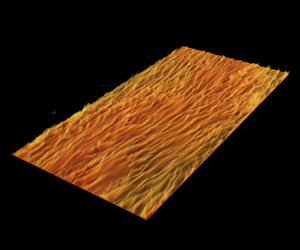
Figure 3. A 3-D representation of the premultiplied spectrum of the convective flux. The slices of normalized 2-D spectra ( $(k_x k_y \phi _{u_z \theta,u_z \theta }) H^{2} / U_F \varDelta$) taken at mid-height and the thermal BL height are shown along with the normalized 1-D premultiplied spectra along the streamwise ( $(k_x \phi _{u_z \theta,u_z \theta }) H / U_F \varDelta$) and spanwise ( $(k_y \phi _{u_z \theta,u_z \theta }) H / U_F \varDelta$) directions. The locations of the primary and secondary peaks corresponding to the superstructures and the small-scale structures are indicated with blue and red lines, respectively. The separation between the scales is indicated with the green line. Contours containing half of the spectral energy are indicated with cyan coloured curves in these slices.
The volume visualisation of the normalized 2-D premultiplied spectra of the convective flux  $(k_x k_y \phi _{u_z \theta,u_z \theta }) H^{2} / U_F \varDelta$ for $1/Ri = 1.0$ is shown in figure 3. Two high-energy regions corresponding to the low wavenumber superstructures and high wavenumber small-scale structures are observed. Since a larger separation of scales indicates stronger turbulence, we hypothesize that the scale separation between the superstructures and small-scale structures is a measure for the turbulence inside the BLs.
Figure 4 shows the premultiplied 2-D spectra of the convective flux ( $k_x k_y \phi _{u_z \theta,u_z \theta }$) computed at mid-height and the thermal BL height. The plots (i-a)–(viii-a) show two distinct high-energy regions. The coloured contours enclose half of the total spectral energy and the colours are indicative of the $1/Ri$ as they vary from red for $1/Ri = 0$ to blue for $1/Ri = 10$. The marker indicates the location of the secondary high-energy region corresponding to the small-scale structures. It is difficult to indicate a similar location for the low wavenumber high-energy region because of the lack of fully converged data. The time scales of these large-scale flow structures are very large and it is computationally very expensive to time average for a sufficient interval of time to obtain fully converged spectra in this low wavenumber region. The high-energy region at low wavenumbers corresponds to thermal superstructures, while the high-energy region at the high wavenumbers corresponds to the small-scale flow structures. As the shear imposed on the system increases, the separation between the superstructures and small-scale structures increases. This is demonstrated by the half-energy contours being ‘stretched’ more and more as $1/Ri$ increases from 0 to 10. The plots (i-b)–(vii-b) show that the secondary high-energy region is dominant at the thermal BL height. The plots (i-c)–(viii-c) and (i-d)–(viii-d) show that the secondary high-energy region occurs very close to the thermal BL height.
In order to better understand the difference in the separation between the primary and secondary peaks with increasing wall shear, we plot the half-energy contours and the location of the peaks taken from figure 4(i-a)–(viii-a) in figure 5(a) and we plot the half-energy contours and the location of the peaks taken from figure 4(i-b)–(viii-b) in figure 5(b). Although figure 5(a) shows that the variation with  $1/Ri$ in the location of the secondary peaks at mid-height is minimal, figure 5(d) clearly shows that the separation of scales at the thermal BL height attains a minimum for $1/Ri = 1.0$, coinciding with the minimum in $Nu$ shown in figure 1. Although we can not point out the exact location of the primary peaks, it is to be noted that they are very close to the origin. Therefore, the separation between the scales of these flow structures is essentially the distance between the origin and the indicated markers. Also note that the wavenumbers for figure 5(d) are normalized with the domain length and width while the wavenumbers for figure 5(a) are normalized with the domain height. For the spectra computed at the thermal BL height, the influence of the domain size on structures is more prominent than at the mid-height due to the stronger effect of shear. Therefore, at the thermal BL height it is more useful to look at the wavenumbers normalized with the respective domain sizes rather than with the domain height. The high-energy region also shrinks in size as the shear increases from $1/Ri = 0$ to $1/Ri = 1.0$ where the secondary high-energy region is smallest. Beyond this point, the region again grows as the applied shear forcing increases from $1/Ri=1.0$ to $1/Ri=10.0$. A larger separation of scales in the convective flux indicates a wider range of sizes in the flow structures contributing to the heat transfer, suggesting that the thermal BL is more turbulent. The variation in the bulk is less pronounced as the bulk offers a thermal ‘shortcut’ at the $Ra$ and $Pr$ considered here (Grossmann & Lohse Reference Grossmann and Lohse2000, Reference Grossmann and Lohse2001, Reference Grossmann and Lohse2002, Reference Grossmann and Lohse2004; Stevens et al. Reference Stevens, van der Poel, Grossmann and Lohse2013). Clearly, the heat flux through the BL is the bottleneck for the total heat flux through the system for the range of $Ri$ considered here.

Figure 4. (i-a)–(viii-b) Two-dimensional premultiplied spectra of the convective flux. The coloured contours represent the envelope containing half of the total spectral energy. One-dimensional premultiplied spectra of the convective flux along the (i-c)–(viii-c) streamwise direction and (i-d)–(viii-d) spanwise direction. The dashed line indicates the thermal BL height. The location of the secondary peak corresponding to the small-scale structures is shown with the coloured markers. The colours of the markers and contours correspond to various  $1/Ri$ as listed in the legend of figure 5.

Figure 5. (a) Contours of normalized 2-D premultiplied convective spectra  $k_x k_y \phi _{u_z \theta, u_z \theta } H^{2} / U_F \varDelta$ taken from figure 4(i-a)–(viii-a) and (d) contours of normalized 2-D premultiplied convective spectra $k_x k_y \phi _{u_z \theta, u_z \theta } L_x L_y / U_F \varDelta$ taken from figure 4(i-b)–(viii-b) containing half of the total spectral energy. Corresponding 1-D premultiplied spectra of the convective flux at mid-height for various $1/Ri$ plotted against the (b,e) streamwise and (c, f) spanwise wavenumber. The markers represent the location of the small-scale structure peak. Note the different scales in (a–c) and (d–f); see details in text. The location of the peaks corresponding to the superstructures is very close to the origin. Therefore, the separation between the scales of these flow structures is essentially the distance between the origin and the indicated markers.
In addition to the separation of scales, figures 5(b), 5(c) and 5(e) show that the energy contained in the secondary peak shows a similar trend as  $Nu$. With an increase in $1/Ri$, the height of the secondary peaks in figures 5(b), 5(c) and 5(e) initially decrease, attain a minimum for $1/Ri=1.0$ and increase again up to $1/Ri=10.0$. Note that the markers indicating the location of the secondary peak do not completely collapse with the location of the secondary peak in figures 5(b) and 5(c) because the marker indicates the secondary peak of the 2-D spectra as shown in figure 4. The streamwise and spanwise 1-D spectra in figures 5(b) and 5(c) are obtained by integrating the 2-D spectra from figure 4 in the spanwise and streamwise directions, respectively. The peak of the integrated 1-D spectra is at a slightly different location than the peak in the parent 2-D spectra from which it was derived. Therefore, there is a small difference in the location of the secondary peak of the 1-D and 2-D spectra; therefore, the markers in figures 5(b) and 5(c) do not always fall on the peak. This also holds true for figures 7(b) and 7(c).
Figure 6 shows the time-averaged premultiplied spectra of turbulent kinetic energy. The normalized turbulent kinetic energy represents the amount of kinetic energy contained in the turbulent fluctuations in comparison with the kinetic energy supplied through the shear forcing. At the thermal BL height, the normalized kinetic energy should be a good indicator of the effectiveness of the applied shear forcing in making the thermal BL more turbulent. In figure 6(i-a)–(vii-b) the secondary peaks are prominent and follow a similar locus of travel in the wavenumber space with variation in  $1/Ri$ as the secondary energy peaks in the convective flux spectra. The variation is clearer in figures 7(a) and 7(d) with the strength of the secondary peak dominating the energy distribution at the thermal BL height as shown in figures 7(e) and 7( f).

Figure 6. (i-a)–(viii-b) Two-dimensional premultiplied spectra of the normalized turbulent kinetic energy. The coloured contours represent the envelope containing half of the spectral energy. Corresponding 1-D premultiplied spectra along the (i-c)–(viii-c) streamwise and (i-c)–(viii-c) spanwise direction. The dashed line indicates the location of the thermal BL height. The location of the secondary peak corresponding to the small-scale structures is indicated by the coloured markers. The colours of the markers and contours correspond to various  $1/Ri$ as listed in the legend of figure 5.

Figure 7. (a) Contours of normalized turbulent kinetic energy  $(k_x k_y \phi _{k,k}) H^{2} / u_{\tau }^{2}$ taken from figure 6(i-a)–(viii-a) and (d) contours of normalized turbulent kinetic $(k_x k_y \phi _{k,k}) L_x L_y / u_{\tau }^{2}$ taken from figure 6(i-b)–(viii-b), containing half of the total spectral energy. Corresponding 1-D spectra at mid-height for various $1/Ri$ plotted against the (b,e) streamwise and (c, f) spanwise wavenumber. The markers indicate the location of the secondary peak corresponding to the small-scale structures.
One wonders whether for strong shear Lumley-type scaling (Lumley Reference Lumley1967; Lohse Reference Lohse1994; Biferale & Procaccia Reference Biferale and Procaccia2005)  $E_u (k) \sim k^{-7/3}$ and $E_\theta (k) \sim k^{-4/3}$ for the velocity and temperature spectrum may show up in our spectra. Note that here k indicates the the wave number. However, those theoretical predictions were made for homogeneous turbulent shear flow. Given the plates, the detachment of plumes from them, and the relatively low Reynolds numbers we can numerically treat and the correspondingly short inertial range, we do not expect to see pronounced Lumley-type shear in our data. This is confirmed by the 1-D velocity and temperature spectra included in the online supplementary material available at https://doi.org/10.1017/jfm.2022.425.
5. Coherence spectra of convective flux and turbulent kinetic energy
The correlation between the heat transfer and the strength of turbulent kinetic energy can be investigated further by studying the coherence spectra between the normalized turbulent kinetic energy and convective flux ( $\gamma ^{2}_{u_z \theta, k}$), which is defined as
 \begin{equation} \gamma^{2}_{u_z \theta, k}(k_x, k_y, z) = \frac{\phi_{u_z \theta, k}(k_x, k_y, z)}{\phi_{u_z \theta, u_z \theta} (k_x, k_y, z)\phi_{k, k}(k_x, k_y, z)}, \end{equation}
with  $\phi _{u_z \theta, k}$ representing the co-spectra of the convective flux and turbulent kinetic energy. Figure 8(i-a)–(vii-b) shows that the wavenumbers corresponding to high-energy regions enclosing the small-scale peak of the convective flux (represented with the solid contours) are very similar to those of the turbulent kinetic energy (shown with the dotted contours). The location of the secondary peaks of the convective flux spectra (represented with the circular and diamond markers) are almost coincident with those of the turbulent kinetic energy spectra (shown with plus and star markers). The coherence between the convective flux and turbulent kinetic energy is relatively high in these regions. Figure 8(i-c)–(viii-d) shows that the coherence at the BL height is very similar for the large- and small-scale flow structures. This shows that there is a strong correlation between the turbulent kinetic energy and the convective heat flux in the BLs.

Figure 8. (i-a)–(viii-b) Coherence spectra between the convective flux and normalized turbulent kinetic energy. The dotted curve indicates the half-energy contours of the convective flux taken from figure 4(i-a)–(viii-b), and the solid curve indicates the half-energy contours of the turbulent kinetic energy taken from figure 6(i-a)–(viii-b). The markers are consistent with the legends in figures 5 and 7. Corresponding 1-D spectra along the (i-c)–(viii-c) streamwise and (i-d)–(viii-d) spanwise direction. The dashed line represents the thermal BL height.
This strong correlation is also suggested by figure 9(b), which shows the wall-normal turbulent kinetic energy profile, averaged in time and horizontal directions and normalized with  $u_{\tau }^{2}$. It can be seen that this ratio of turbulent kinetic energy to the kinetic energy imparted through shear is lowest in the BL for $1/Ri = 1.0$ when $Nu$ is lowest.

Figure 9. (a) Thermal BL thickness ( $\lambda _\theta$) and kinetic BL thickness ( $\lambda _u$) vs wall Reynolds number. (b) The turbulent kinetic energy normalized with the square of the friction velocity plotted against wall-normal coordinate. Both plots correspond to $\varGamma _x = 48$, $\varGamma _y = 24$.
6. Effect of shear on large-scale structures
This reduction in the turbulence level in the thermal BL may be attributed to the following phenomena. The buoyancy-driven plumes responsible for the turbulent convective transport of heat are ejected from the thermal BLs (Ahlers, Grossmann & Lohse Reference Ahlers, Grossmann and Lohse2009) and impact the opposite BL. In sheared RB the plumes carry heat and momentum. This momentum is small for lower imposed wall velocities. In this regime, the kinetic BL is much thicker than the thermal BL, due to which the plumes carry a relatively large fraction of the momentum imposed by the wall. For higher imposed wall velocities, the kinetic BL is thinner, and the fraction of the momentum of the wall that is transferred to the plumes is relatively low. However, this is compensated by the larger wall velocity. Around  $1/Ri = 1.0$, the thickness of the kinetic BL ( $\lambda _u$) is only slightly larger than the thickness of the thermal BL ( $\lambda _\theta$) as seen in figure 9(a), and the wall velocity is not high enough to energize the plumes sufficiently to enhance $Nu$.
$Nu$.
The change in the BL dynamics can also be observed in figure 10. Figure 10(i-a)–(viii-a) shows the probability density plot of the local horizontal flow velocity with respect to the imposed wall velocity as a function of the normalized height from the wall ( $z/\lambda _{\theta }$). Figure 10(i-b)–(viii-b) shows the corresponding plot for the local horizontal component of velocity with the temporally and spatially averaged mean subtracted. The probability densities are defined as
 \begin{equation} \psi_{u_x,u_y}(\alpha) = \frac{N(\alpha-\delta \leq \alpha(u_x,u_y) < \alpha+\delta)}{2 N_G \delta} \quad \forall\ \alpha \in \{-{\rm \pi}, -{\rm \pi}+2\delta, -{\rm \pi}+4\delta,\ldots{\rm \pi}\} \end{equation}
and
 \begin{align}
\psi_{u_x^{\prime},u_y^{\prime}}(\alpha) =
\frac{N(\alpha-\delta \leq
\alpha(u_x^{\prime},u_y^{\prime}) < \alpha+\delta)}{2 N_G
\delta} \quad \forall\ \alpha \in \{-{\rm \pi}, -{\rm \pi}+2\delta,
-{\rm \pi}+4\delta,\ldots{\rm \pi}\},
\end{align}
\begin{align}
\psi_{u_x^{\prime},u_y^{\prime}}(\alpha) =
\frac{N(\alpha-\delta \leq
\alpha(u_x^{\prime},u_y^{\prime}) < \alpha+\delta)}{2 N_G
\delta} \quad \forall\ \alpha \in \{-{\rm \pi}, -{\rm \pi}+2\delta,
-{\rm \pi}+4\delta,\ldots{\rm \pi}\},
\end{align}
with  $N(\cdots )$ indicating the number of grid points satisfying the condition inside the parenthesis, $N_G$ indicating the total number of grid points at a given height $z$, and
 \begin{equation} u_x^{\prime} = u_x - \left\langle u_x \right\rangle_{A,t},\quad u_y^{\prime} = u_y - \left\langle u_y \right\rangle_{A,t}. \end{equation}
The angle  $\alpha (u_x,u_y)$ is defined as the angle subtended by the vector $(u_x,u_y,0)$ with $(-U_w,0,0)$ if the grid point under consideration lies in the bottom half of the domain. For grid points in the top half of the domain, $\alpha (u_x,u_y)$ is defined as the angle subtended by the vector $(u_x,u_y,0)$ with $(U_w,0,0)$. The angle $\alpha (u_x^{\prime },u_y^{\prime })$ is also defined similarly. The value of $\delta$ is chosen to be ${\rm \pi} /72$.

Figure 10. (i-a)–(viii-a) Probability density function given by (6.1), as a function of the angle subtended by the local horizontal component of the velocity with the streamwise direction ( $\alpha$), plotted against height from the wall normalized by the BL height ( $z/\lambda _{\theta }$). (i-b)–(viii-b) Probability density function of the fluctuations of the horizontal components of the velocity given by (6.2). The white dashed line indicates the thermal BL height. (i-c)–(viii-c) Probability density function of $\psi (\alpha )$ for the horizontal components and their fluctuations at mid-height and thermal BL height.
In both cases, a prominent high probability density region is observed for  $\alpha \approx {\rm \pi}/2$ just above the thermal BL height. This region has the highest probability density for $1/Ri = 1.0$, which shows that the velocity induced at the thermal BL height by the large-scale superstructures or plumes is primarily oriented in a direction perpendicular to that of the wall velocity, indicating that at $1/Ri = 1.0$ the imposed shear is least effective at making the thermal BLs more turbulent. A more thorough investigation involving conditional averaging of the momentum carried by the plumes, similar to the study performed in Blass et al. (Reference Blass, Verzicco, Lohse, Stevens and Krug2021b), could further strengthen this view. Future studies are planned to filter out the smaller scales to study the orientation of these larger heat-carrying plumes and the ‘wind of turbulence’ (Castaing et al. Reference Castaing, Gunaratne, Heslot, Kadanoff, Libchaber, Thomae, Wu, Zaleski and Zanetti1989; Grossmann & Lohse Reference Grossmann and Lohse2000) imparted by these plumes to the thermal BL.
7. Effect of domain size on Nusselt number
To further confirm that the flow structures corresponding to the secondary peaks are critical for the heat transport, we progressively reduce the domain size of the simulations to assess how this affects  $Nu$. Figure 11 shows that the changes in the variation of $Nu$ are minor until the domain is no longer large enough to contain the smaller flow structures associated with the secondary peak. It can be seen that a domain of aspect ratio $\varGamma _x = 1.0$, $\varGamma _y = 0.5$ is necessary to accommodate the secondary peak for most of the $Ri$ cases considered. As soon as the domain aspect ratio is reduced to $\varGamma _x = 0.6$, $\varGamma _y = 0.3$ $Nu$ drops drastically. Similar observations can be made on the variation of $Re_{\tau }$ with $Re_w$. As soon as the domain aspect ratio is reduced to $\varGamma _x = 0.6$, $\varGamma _y = 0.3$, we observe that $Re_{\tau }$ drops drastically. This observation of the minimal sheared RB domain is similar to the minimal Couette flow study performed by Sekimoto, Atkinson & Soria (Reference Sekimoto, Atkinson and Soria2018) and the minimal channel flow study by Jiménez & Moin (Reference Jiménez and Moin1991). The minimum domain size required to obtain the $Nu$ and $Re_{\tau }$ values associated with laterally unconfined sheared RB flow is a function of the shear and thermal driving. However, the fact that the domain must be sufficiently large to accommodate these small-scale structures associated with the secondary peaks is a valuable observation for reducing the computational costs of simulations focusing on the heat transport phenomena.

Figure 11. (a) Boxes showing the domain sizes overlaid on the contours from figure 5(d). (b) Plot of  $Nu$ as a function of $Re_w$ for various domain sizes. (c) Plot of $Re_{\tau }$ as a function of $Re_w$ for various domain sizes.
8. Conclusions
Complimentary to previous studies (Blass et al. Reference Blass, Zhu, Verzicco, Lohse and Stevens2020, Reference Blass, Tabak, Verzicco, Stevens and Lohse2021a), which focus on how the large-scale dynamics affect  $Nu$, we focus on effects of small-scale flow structures at the BL. Since the bulk offers a thermal ‘shortcut’ for the range of parameters considered in the study, the BL dynamics determine the heat transfer in the system. This follows from the analysis of the spectra of convective flux and turbulent kinetic energy, which shows the presence of the spectral peaks corresponding to large-scale superstructures and small-scale structures. We observe that the separation of scales between these superstructures and small-scale structures at the thermal BL is indicative of the ratio between the turbulent kinetic energy in the thermal BL and the square of the friction velocity. A larger separation between superstructures and small-scale structures at the thermal BL height is directly correlated to a more turbulent thermal BL and a higher $Nu$. We also observe the minimum $Nu$ occurs at $1/Ri=1.0$ along with the smallest separation between superstructures and small-scale structures as well as the lowest normalized turbulent kinetic energy at the thermal BL height. The strong coherence between the small-scale structures of convective flux and turbulent kinetic energy spectra at the thermal BL height, which is similar in magnitude to that of the superstructures in the bulk, confirms that the convective heat transfer is closely related to the turbulent kinetic energy within the BLs.
Although the fluctuations of velocity in the thermal BL are imparted by the large-scale ‘wind of turbulence’ consisting of plumes travelling through the bulk, the orientation of these plumes impacting the BLs is determined by the momentum carried by these plumes, which, in itself, is a consequence of the BL dynamics. From probability density plots computed using (6.1), (6.2) and shown in figure 10, we observe that the momentum of the wall shear carried by the impacting plumes is lowest for  $1/Ri = 1.0$, which is also the case with lowest $Nu$. We confirm that overall heat transfer is lowest when the applied wall shear is least effective in turning the BLs turbulent, as shown by the smallest separation between the spectral peaks of convective flux and turbulent kinetic energy at the thermal BL height for $1/Ri = 1.0$.
We find that the variation of  $Nu$ and $Re_{\tau }$ in sheared RB convection with domain size is limited as long as the small-scale structures associated with the secondary peaks of the convective flux and turbulent kinetic energy spectra is captured. We find that, for the parameter regime under consideration, a domain size of $\varGamma _x = 1.0$, $\varGamma _y = 0.5$ is sufficient to achieve this. We note that the identification of a minimal system size that captures the leading dynamics in sheared convection is analogous to the concept of minimal span Couette flow studies performed by Sekimoto et al. (Reference Sekimoto, Atkinson and Soria2018), and the study on minimal channel flow by Jiménez & Moin (Reference Jiménez and Moin1991) which, in turn, support the inference that the large domains that fully capture the superstructures are not required to obtain the converged values of $Nu$ and $Re_{\tau }$.
Supplementary material
Supplementary material is available at https://doi.org/10.1017/jfm.2022.425.
Acknowledgements
The authors gratefully acknowledge C.S. Ng, C. Howland, A. Blass and R. Hartmann for fruitful discussions.
Funding
This work was financially supported by the ERC starting grant (2018) for the project ‘UltimateRB’ and the Twente Max-Planck Center. We acknowledge PRACE for awarding us access to MareNostrum at Barcelona Supercomputing Center (BSC), Spain (Project 2020225335 and 2020235589). The simulations were also supported by a grant from the Swiss National Supercomputing Centre (CSCS) under project ID s997. This work was carried out on the Dutch national e-infrastructure with the support of SURF Cooperative.
Declaration of Interests
The authors report no conflict of interest.
Appendix. Numerical simulations
Table 1. Simulations considered in this work. The aspect ratio of the domain is given by  $\varGamma _x$ in the streamwise direction and $\varGamma _y$ in the spanwise direction. The values of $N_x$, $N_y$ and $N_z$ indicate the number of grid points in the streamwise, spanwise and wall-normal directions. The grid spacing in wall units in the streamwise and spanwise directions is given by $\Delta x^{+}$ and $\Delta y^{+}$, respectively. The wall-normal grid spacing in wall units at the wall and the mid-height is given by $\Delta z_w^{+}$ and $\Delta z_c^{+}$, respectively. The number of grid points in the wall-normal direction within the thermal BL is given by $N_{BL}$. The values of $Re_{\tau }$ and $Nu$ are averaged for the duration of the non-dimensional time given by either $t_{avg}/t_{ff}$, where $t_{ff} = \sqrt {H/g \beta \varDelta }$ is the free fall velocity, or by $t_{avg} u_{\tau } / \lambda _u$.


 Open access