


1. Introduction
Channelized particle–fluid flows are common in industry and nature, from particle–slurry transport in processing industries, to rivers and gravity-driven particle–fluid flows in nature. Theoretical and experimental studies have demonstrated how even subtle channel width variations significantly influence flow dynamics of Newtonian fluids (Chester Reference Chester1953; Chen & Capart Reference Chen and Capart2020). Studies of natural flows have demonstrated that channel width non-uniformities influence not only fluid dynamics but also associated sediment erosion, sediment deposition and associated morphodynamics (Ferrer-Boix et al. Reference Ferrer-Boix, Chartrand, Hassan, Martín-Vide and Parker2016; Chartrand et al. Reference Chartrand, Jellinek, Hassan and Ferrer-Boix2018; Saletti & Hassan Reference Saletti and Hassan2020). For flows of higher sediment concentrations, e.g. in gravity-driven debris flows, numerical models suggest that non-uniform width channels also affect the flow dynamics (Schilirò et al. Reference Schilirò, De Blasio, Esposito and Scarascia Mugnozza2015), though these studies are significantly more limited. Compared to water flows in engineered or natural channels, the constitutive laws needed to predict the response of high-solid-fraction particle–fluid flows to complex stresses have not yet reached a sufficient level to predict the response of these flows to arbitrarily changing widths.
In the last few decades, significant progress has been made towards capturing specific aspects of natural particle–fluid flows. These have included depth-averaged models with relatively simple friction laws (Savage & Hutter Reference Savage and Hutter1989; Gray Reference Gray2001), and experiments and simulations capturing more complex rheologies of dry granular flows (i.e. via an ‘inertial number’  $I$) (GDR-MiDi 2004; da Cruz et al. Reference da Cruz, Emam, Prochnow, Roux and Chevoir2005; Forterre & Pouliquen Reference Forterre and Pouliquen2008; Yohannes & Hill Reference Yohannes and Hill2010). Combined, these provide the framework for depth-averaged models using more representative rate-dependent friction rules (Iverson Reference Iverson2012). When wall friction was properly accounted for (Taberlet et al. Reference Taberlet, Richard, Valance, Losert, Pasini, Jenkins and Delannay2003; Jop, Forterre & Pouliquen Reference Jop, Forterre and Pouliquen2006), Capart, Hung & Stark (Reference Capart, Hung and Stark2015) showed that this combination successfully predicts flow behaviour in uniform-width channels by considering kinetic energy balance in addition to mass and momentum. Numerical modelling efforts have been supplemented by laboratory experiments in different configurations. In particular, rotating drums have been used to study dry granular flows over a wide range of regimes (Ristow Reference Ristow1996; Gray Reference Gray2001; Amon, Niculescu & Utter Reference Amon, Niculescu and Utter2013), as well as debris flows (Kaitna, Rickenmann & Schatzmann Reference Kaitna, Rickenmann and Schatzmann2007; Hsu, Dietrich & Sklar Reference Hsu, Dietrich and Sklar2014). In this paper, we focus on dry free-surface granular flows as they transition from continuous slow flows to cascading flows (Orpe & Khakhar Reference Orpe and Khakhar2001; Félix, Falk & D'Ortona Reference Félix, Falk and D'Ortona2007; Pignatel et al. Reference Pignatel, Asselin, Krieger, Christov, Ottino and Lueptow2012; Hung, Stark & Capart Reference Hung, Stark and Capart2016). To do so, we build on the theoretical framework of our previously developed depth-averaged model. We then use this to consider explicitly the influence of curved walls on advection and dissipation of kinetic energy, and investigate how various mechanisms change with channel geometry and drum rotation rate. We test the model by performing a series of dry granular flow experiments in concave and convex rotating drums.
2. Theory
Our theoretical boundary conditions, illustrated in figure 1(a), involve steady granular surface flows in channels of varying width  $B(x)$. The flow surface ${\tilde {z}}(x)$ is of varying inclination $\beta (x)$. The granular shear flow extends down to a theoretical basal boundary ${\underset{\sim}{z}}(x)$ that we model as a yield surface, at and below which there is no shearing ( $\dot {\gamma } = 0$ at $z = {\underset{\sim}{z}}$). Following Liggett (Reference Liggett1994), we denote variable values sampled at the free surface and bottom boundary using tildes above and below the variables, respectively. For simplicity, we consider coordinate axes $(x,z)$ inclined at a constant angle of repose $\alpha$, rather than curvilinear coordinates fitted to the actual free surface. In the model, the geometry of the free surface is therefore approximated by profile ${\tilde {z}}(x)$, such that $S(x) = \tan (\beta (x)-\alpha ) = -{\rm d} {\tilde {z}} /{{\rm d}\kern0.7pt x}$ represents an excess slope, positive where $\beta (x)>\alpha$, and negative where $\beta (x)<\alpha$.

Figure 1. Definition sketches illustrating the components of this research. (a) Steady granular surface flow in channel of non-uniform width forced by a steady upward current at the base. (b) Half-filled rotating drum configuration used to test the theory. (c) Assumed flow kinematics with solid-body rotation with the drum below the basal yield surface (blue streamlines). Grey streamlines illustrate the movement of the particles as they would be if they did not flow with gravity but rather continued in solid-body rotation throughout the circulation. (d) Sketch of one experimental drum. In (b,c), the velocities and streamlines are shown in a stationary (non-rotating) frame of reference.
Our simplifying assumptions are as follows. We approximate the flows as shallow, gradually varying in the longitudinal direction  $x$, and subject to hydrostatic pressure variations in the $z$-direction. We neglect dilation effects (Delannay et al. Reference Delannay, Louge, Richard, Taberlet and Valance2007), and approximate the density of the flow layer as uniformly dense, of constant bulk density $\rho$, and subject to a linearized version of the $\mu (I)$ rheology (da Cruz et al. Reference da Cruz, Emam, Prochnow, Roux and Chevoir2005; Jop, Forterre & Pouliquen Reference Jop, Forterre and Pouliquen2005). For steady drum flows, some of these assumptions become less valid as the rotation rate increases, but we will nevertheless adopt them and re-assess when comparing model results with experiments.
We start with a general expression for mass balance, averaged over the local width  $B(x)$:
 \begin{equation} \frac{\partial \rho uB}{\partial x} + \frac{\partial \rho wB}{\partial z} = 0. \end{equation}
Here,  $u(x,z)$ and $w(x,z)$ are the $x$- and $z$-components of the velocities, averaged over the channel width between $y=0$ and $y=B$. Upon approximating the bulk density $\rho$ as uniform and constant, we rewrite (2.1) as
 \begin{equation} \frac{u}{B}\,\frac{{\rm d} B}{{\rm d}\kern0.7pt x}+\frac{\partial u}{\partial x}+\frac{\partial w}{\partial z} = 0. \end{equation}
Similarly, we express the steady state width-averaged  $x$-momentum balance as
 \begin{equation} \frac{u^2}{B}\,\frac{{\rm d} B}{{\rm d}\kern0.7pt x}+u\,\frac{\partial u}{\partial x} + w\,\frac{\partial u}{\partial z} = \frac{1}{\rho}\,\frac{\partial \sigma}{\partial x}+\frac{1}{\rho}\,\frac{\partial \tau}{\partial z}-2\,\frac{\tau_B}{\rho B}+g_{x}. \end{equation}
Here,  $g_x = g \sin \alpha$, $\sigma$ and $\tau$ are normal and shear stresses ( $-\sigma _{zz}$ and $\sigma _{zx}$ in the Cauchy stress tensor), and $\tau _B$ is a sidewall frictional stress. Following Jop et al. (Reference Jop, Forterre and Pouliquen2006), we approximate $\sigma$ as isotropic and neglect acceleration in the $z$-direction, so that
 \begin{equation} 0 = \frac{1}{\rho}\,\frac{{\rm d} \sigma}{{\rm d}z} + g_z, \end{equation}
where  $g_z = g \cos \alpha$. Assuming $\tilde {\sigma } = 0$ at the free surface then yields $\sigma (z) = \rho g_z \eta$, where $\eta = \tilde {z} - z$. For $\tau$, we adopt the linearized rate-dependent $\mu (I)$ rheology (da Cruz et al. Reference da Cruz, Emam, Prochnow, Roux and Chevoir2005; Capart et al. Reference Capart, Hung and Stark2015; Hung et al. Reference Hung, Stark and Capart2016):
 \begin{equation} \tau = \mu(I)\,\sigma = ( \mu_0 + \chi I) \sigma. \end{equation}
We take  $\mu _0 = \tan \alpha$; the product $\mu _0 \sigma$ serves as a rate-independent, pressure-dependent yield stress. Parameter $\chi$ is a dimensionless rheological coefficient that can be determined from steady chute flow experiments (Capart et al. Reference Capart, Hung and Stark2015). The dimensionless number $I$ is the inertial number defined by $I = \dot {\gamma } d \sqrt {\rho /\sigma }$, where $d$ is the mean particle diameter, and $\dot {\gamma } = -\partial u/\partial z$ is the shear rate. We approximate the wall shear stress by $\tau _B = \mu _B \sigma$, following the Coulomb friction rule (Taberlet et al. Reference Taberlet, Richard, Valance, Losert, Pasini, Jenkins and Delannay2003; Jop et al. Reference Jop, Forterre and Pouliquen2005, Reference Jop, Forterre and Pouliquen2006). The particle–wall friction coefficient $\mu _B$ is assumed constant, independent of flow velocity $u$ and location $(x,z)$.
Next, we use a depth-averaging approach to simplify our equations, making the problem more tractable and the ensuing behaviours more transparent. We integrate (2.2) over the shearing layer to obtain the width- and depth-averaged mass conservation expression for the shearing layer:
 \begin{equation} \int^{{\tilde{z}}}_{{\underset{\sim}{z}}} \left( \frac{u}{B}\,\frac{{\rm d} B}{{\rm d}\kern0.7pt x}+\frac{\partial u}{\partial x}+\frac{\partial w}{\partial z} \right) \,{\rm d}z = \frac{h \bar{u}}{B}\,\frac{{\rm d} B}{{\rm d}\kern0.7pt x} + \frac{\partial}{\partial x} (h \bar{u}) - {\tilde{u}}\,\frac{\partial {\tilde{z}}}{\partial x} + {\tilde{w}} -{\underset{\sim}{w}} = 0. \end{equation}
For the theoretical derivation, we set the  $x$-component of the velocity at the basal boundary ${\underset{\sim}{u}} = u({\underset{\sim}{z}}) =0$. Then in (2.6), $\bar {u}$ is the velocity in the $x$-direction, averaged over both width and depth, and ${\tilde {w}}$ and ${\underset{\sim}{w}}$ are the velocities in the $z$-direction, averaged over width at the free surface and at the basal boundary, respectively. Thus ${\underset{\sim}{w}}=w({\underset{\sim}{z}})$ represents a current of grains normal to the flow layer, acting as a source if ${\underset{\sim}{w}}>0$ and as a sink if ${\underset{\sim}{w}}<0$. The corresponding volume transfer between the substrate and the flow layer is analogous to what occurs when a granular flow erodes ( $\partial {\underset{\sim}{z}}/\partial t < 0$) a stationary bed ( ${\underset{\sim}{w}}=0$). When upward current and downward erosion occur simultaneously, the transfer rate at the base is given by $e = {\underset{\sim}{w}} - \partial {\underset{\sim}{z}}/ \partial t$ (Hung, Aussillous & Capart Reference Hung, Aussillous and Capart2018), and when only erosion occurs, it is given by $e= -\partial {\underset{\sim}{z}}/ \partial t$ (Capart et al. Reference Capart, Hung and Stark2015).
Along the free surface, we invoke the kinematic boundary condition  $\partial {\tilde {z}}/\partial t + {\tilde {u}}\,\partial {\tilde {z}} / \partial x =$ ${\tilde {w}}$. For steady-state conditions, we can then write the depth-averaged mass balance equation as
 \begin{equation} \frac{1}{B}\,\frac{{\rm d}}{{\rm d}\kern0.7pt x}(B h \bar{u}) = {\underset{\sim}{w}}. \end{equation}
Similarly, we integrate the momentum equation over depth. In doing so, we relate the second moment of the velocity to the first ( $\bar {u}^2$ to $\overline {u^2}$) using the self-similar velocity profile solution for constant-width channels (Tsubaki, Hashimoto & Suetsugi Reference Tsubaki, Hashimoto and Suetsugi1982; Berzi & Jenkins Reference Berzi and Jenkins2008):
 \begin{equation} u(x,z) = \bar{u}(x)\,f(\hat{\eta}) = \bar{u}(x) \left(\frac{7}{3} - \frac{35}{6}\,\hat{\eta}^{{3}/{2}} + \frac{7}{2}\,\hat{\eta}^{{5}/{2}}\right), \end{equation}
where  $\hat {\eta }(x)=({\tilde {z}}(x)-z)/h(x)$. Using this, and the relationships for stresses discussed above, we can express the depth-averaged momentum equation as
 \begin{equation} \frac{1}{B}\,\frac{{\rm d}}{{\rm d}\kern0.7pt x}(\kappa_0 h \bar{u}^2 B) ={-}h g_z\,\frac{{\rm d} {\tilde{z}}}{{\rm d}\kern0.7pt x} - \frac{\mu_B}{B}\,h^2 g_z, \end{equation}
where  $\kappa _0=77/48$. From the work above, we have three unknown variables ${\tilde {z}}(x), h(x), \bar {u}(x)$, one unspecified boundary condition $\underset{\sim}{w}(x)$, and only two governing equations ((2.7) and (2.9)). To help close this, we derive a depth-averaged kinetic energy equation as in Capart et al. (Reference Capart, Hung and Stark2015), by multiplying both sides of (2.3) by the local velocity $u(x,z)$ and integrating it across the shear layer:
 \begin{equation} \frac{1}{B}\,\frac{{\rm d}}{{\rm d}\kern0.7pt x}\left( \kappa_1 h \bar{u}^3 B \right) ={-} h \bar{u} g_z\,\frac{{\rm d}{\tilde{z}}}{{\rm d}\kern0.7pt x} - \kappa_2 \chi d\,\sqrt{h g_z}\,\frac{\bar{u}^2}{h} - \kappa_3\, \frac{\mu_B}{B}\,g_z h^2 \bar{u}, \end{equation}
for which we find  $[\kappa _1,\kappa _2,\kappa _3] = [{342\,853}/{233\,376}, {35}/{9}, {5}/{9}]$ using (2.8). The terms (in order from left to right) account for the downslope kinetic energy flux, kinetic energy production by the pressure gradient, energy dissipation by the granular-viscous stress, and energy dissipation due to wall friction. For the boundary condition ${\underset{\sim}{w}}(x)$, we turn to a specific geometry that we can replicate experimentally: rotated drums with non-uniform, radially symmetric widths.
3. Application to rotating drums
3.1. Experimental parameters
We test the theoretical predictions by measuring steady experimental flows in rotating drums of radius  $R = 200$ mm (figures 1b–d) and non-uniform radially symmetric widths $B=B(r)$, given by the parabolic profile
 \begin{equation} B(r) = B_0 (1+ \lambda (r/R)^2). \end{equation}
Here,  $B_0=B(0)$, and dimensionless parameter $\lambda$ controls the width variation. For the work described here, we created two new drums with the same radius ( $R=200$ mm) and smallest width (40 mm) as the uniform gap width experiments ( $\lambda = 0)$ conducted by Hung et al. (Reference Hung, Stark and Capart2016) (see table 1). For our two new drums, we machined two new parabolic back plates (illustrated in figures 2a–d). The first ( $B_0 < B(R)$, $\lambda = 1$) exhibits a narrowing gap towards the centre, i.e. concave width variations. The second ( $B_0 > B(R)$, $\lambda = -0.5$) exhibits a widening gap towards the centre, i.e. convex width variations.

Figure 2. Flow fields from (a–d) model predictions and (e–h) experiments, for (a,c,e,g) concave channel, (b,d,f,h) convex channel, with (a,b,e,f)  $\varOmega = 1$ r.p.m., (c,d,g,h) $\varOmega = 10$ r.p.m. Colours indicate velocity magnitude after subtracting the solid-like rotation component; white dashed lines indicate free surface and basal interface; white contour lines are streamlines from level sets of the dimensionless streamfunction $\hat {\psi }$; inclined white lines are centreline transects used to plot velocity profiles in figure 3.

Figure 3. Modelled (lines) and measured (symbols) velocity profiles at the drum centre ( $x = 0$) for concave (blue) and convex (red) drums: (a) $\varOmega = 1$ r.p.m., (b) $\varOmega = 10$ r.p.m. Coloured horizontal lines indicate modelled (continuous) and experimental (dashed) basal depths, the latter determined by excluding 2 % of the discharge in excess of solid body rotation. Error bars indicate the range obtained upon varying this cutoff between 1 % and 4 %. Insets: experimental data plotted on a linear-log scale. Lines represent what exponential decay would look like with decay lengths as indicated from measurements in a heap flow ( $0.72 d$ as in Komatsu et al. Reference Komatsu, Inagaki, Nakagawa and Nasuno2001) and a uniform-width rotated drum ( $1.1 d$ as in Gioia, Ott-Monsivais & Hill Reference Gioia, Ott-Monsivais and Hill2006).
Table 1. Experimental parameters.

Due to differences in materials and fabrication, the surface properties of the different walls are not identical. In all cases, the front wall is flat and made of glass to maximize visual access. Thus the friction coefficient of the front plate is the same for all experiments ( $\mu _{FW}\approx 0.212$). The back plate of the original drum from Hung et al. (Reference Hung, Stark and Capart2016) was made from aluminium, while for ease in manufacturing, the two new back plates were made from acrylic (PMMA). Because the machining processes to make concave and convex shapes were not the same, however, the friction coefficients ( $\mu _{BW}$) for the two back plates also differ.
To estimate friction coefficients for each case, we performed a series of tests using what we call a slider made by gluing five or six particles onto the flat head of a short bolt, with zero, one or two nuts added to vary the weight between 5.2 and 11.8 g. We placed the slider head down at different positions on each plate, laid flat, before we gradually tilted the plate until the slider started to move. We recorded the corresponding inclination and, from this, calculated an approximate normal and tangential force for this condition. For each wall plate, we conducted 15 such tests (three different slider weights at five different positions) and obtained the friction coefficient by linear fit from the normal and tangential forces at the start of sliding. The corresponding values are listed in table 1. For the simulations, we used a single effective particle–wall friction coefficient equal to the average of particle–wall friction coefficients for the front wall and the back wall, as determined from the slider tests.
We use polydisperse aluminosilicate spheres for the experiments, the same as those in the experiments of Capart et al. (Reference Capart, Hung and Stark2015) and Hung et al. (Reference Hung, Stark and Capart2016). Capart et al. (Reference Capart, Hung and Stark2015) determined rheological coefficients  $\mu _0$ and $\chi$ from steady chute flow tests. We use these previously determined values without adjustment for the comparisons between model and experiments, and list them with the other experimental parameters in table 1.
We used a computer-controlled stepper motor to provide stable rotation rates for the drums, ranging from 0.2 to 30 r.p.m. ( $8.92 \times 10^{-6} < Fr < 2.01 \times 10^{-1}$, where $Fr = R \omega ^2/g$ is the (dimensionless) Froude number, and
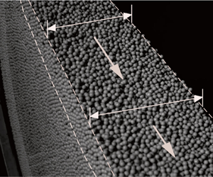
  $\omega$ is the rotation rate in radians per time Mellmann Reference Mellmann2001; Taberlet, Richard & Hinch Reference Taberlet, Richard and Hinch2006). When the half-filled drum is rotated at a constant speed within this range, a shear layer forms (figure 1b), sufficiently shallow that it experiences the width variation primarily in the $x$-direction. (See supplementary movies available at https://doi.org/10.1017/jfm.2022.885.)
3.2. Adaptation of theory to rotating drum boundary conditions
Now we adapt the boundary conditions of the theory to the drum as follows. We approximate  $B$ and ${\underset{\sim}{w}}$ for the shear layer as
 \begin{gather} B(x)=B(0)\,(1+ \lambda (x/R)^2)\quad {{\rm and}} \quad {\underset{\sim}{w}} ={-}\varOmega x, \quad |x| < R, \end{gather}
 \begin{gather} B(x)=0 \quad {{\rm and}} \quad {\underset{\sim}{w}} = 0,\quad |x| \geq R. \end{gather}
Here, we define  ${\underset{\sim}{w}}$ to approximate the normal flux induced by drum rotation across the basal boundary of the flow layer (figure 1b). With these boundary data, the mass balance equation (2.7) can be integrated to
 \begin{equation} Q(x) = Bh\bar{u} = B_0\varOmega\,\frac{R^2-x^2}{2} + \lambda\,\frac{B_0 \varOmega}{R^2}\,\frac{R^4-x^4}{4}. \end{equation}
 To provide insight into the expected flow dynamics, we perform a series of scaling analyses. We first set characteristic scales of  $x$ and $B(x)$: $x_c=R$ and $B_c= B_0$. We substitute these into the energy equation and solve for characteristic scales of $h$,
$h$,  $\bar {u}$ and $S=-{\rm d}{\tilde {z}}/{{\rm d}\kern0.7pt x}$, for which all terms in the energy equation (2.10) are of similar order:
 \begin{equation} h_c = (\chi d)^{1/2}R^{1/4}(B_0/\mu_B)^{1/4}, \quad \bar{u}_c = \left(g_z h_c R (\mu_B /B_0) \right)^{1/2}, \quad S_c = h_c (\mu_B /B_0), \end{equation}
all of which are  $\varOmega$-independent. With this, we define $\hat {x}=x/R$, $\hat {B}=B/B_0$, $\hat {S}=S/S_c$, $\hat {h}=h/h_c$, $\hat {u}=\bar {u}/\bar {u}_c$ and $\hat {S}= S/S_c$, and substitute these into the balance equations (2.7), (2.9) and (2.10). This yields
 \begin{gather} \frac{1}{\hat{B}}\,\frac{{\rm d}}{{\rm d}\hat{x}}\left(\hat{h}\hat{u}\hat{B}\right)={-}\hat{\varOmega}\hat{x}, \end{gather}
 \begin{gather} \frac{\kappa_0}{\hat{B}}\,\frac{{\rm d}}{{\rm d}\hat{x}}\left(\hat{B}\hat{h}\hat{u}^2\right)=\hat{h} \hat S-\frac{\hat{h}^2 }{ \hat{B}}, \end{gather}
 \begin{gather} \frac{\kappa_1}{\hat{B}}\,\frac{{\rm d}}{{\rm d}\hat{x}}\left(\hat{B}\hat{h}\hat{u}^3\right)=\hat{h} \hat{u} \hat S-\frac{\kappa_2\hat{u}^2 }{ \hat{h}} - \frac{\kappa_3 \hat{h}^2 \hat{u}}{ \hat{B}}. \end{gather}
For a given dimensionless width profile  $\hat {B}(\hat {x})$, the only parameter influencing the dynamics is therefore the dimensionless rotation rate $\hat {\varOmega }$ defined by Hung et al. (Reference Hung, Stark and Capart2016) as
 \begin{equation} \hat{\varOmega} = \frac{ \varOmega R^{9/8} \left( B_0/\mu_B \right)^{1/8}}{\sqrt{g_z} \left( \chi d \right)^{3/4}}. \end{equation}
 We next examine two asymptotic regimes for  $\hat {\varOmega }$: $\mathcal {R}_a$ ( $\hat {\varOmega } \to 0$) and $\mathcal {R}_b$ ( $\hat {\varOmega } \to \infty$). We first hypothesize that for the $\mathcal {R}_a$ regime, convection is negligible in the energy equation. To test this, we seek inertia-independent scales [ $h_a, \bar {u}_a, S_a$] for which: (i) the three terms on the right-hand side of (2.10) are of the same order; and (ii) the two terms in (2.7) are as well. We find for these conditions that
 \begin{gather} h_a = (\varOmega R^2)^{2/7} (\chi d)^{2/7} (B_0/\mu_B)^{2/7} g_z^{{-}1/7} = h_c \hat{\varOmega}^{2/7}, \end{gather}
 \begin{gather} \bar{u}_a = (\chi d)^{{-}1} (\mu_B/B_0) g_z^{1/2} h_a^{5/2} = \bar{u}_c \hat{\varOmega}^{5/7}, \end{gather}
 \begin{gather} S_a = (\mu_B/B_0) h_a = S_c \hat{\varOmega}^{2/7}. \end{gather}
We substitute  $\hat {h}_a=h/h_a, \hat {u}_a=\bar {u}/\bar {u}_a$ and $\hat {S}_a= S/S_a$ as well as $\hat x$ and $\hat B$ into the kinetic energy equation (2.10) and find
 \begin{equation} \kappa_1\,\frac{\mathrm{d}}{\mathrm{d}\hat{x}}\left(\hat{B}\hat h_a \hat{u}_a^3 \right)\hat{\varOmega}^{8/7} = \hat{B} \hat h_a \hat{u}_a \hat{S}_a - \kappa_2 \hat{B} \hat h_a^{{-}1/2} \hat{u}_a^2 - \kappa_3 \hat h_a^2 \hat{u}_a . \end{equation}
As we hypothesized, for  $\hat {\varOmega }\to 0$, the kinetic energy flux term is negligible.
For the  $\mathcal {R}_b$ regime ( $\hat {\varOmega }\to \infty$), we test our hypothesis that dissipation by granular-viscous stress is negligible. We thus seek scales [ $h_b, \bar {u}_b, S_b$] for which: (i) all terms of (2.10) except the granular-viscous term are of the same order; and (ii) the two terms in (2.7) are of the same order. We find for these conditions that
 \begin{gather} h_b =(\varOmega R^2)^{2/3} (B_0/\mu_B)^{1/3} R^{{-}1/3} =h_c \hat{\varOmega}^{2/3}, \end{gather}
 \begin{gather} \bar{u}_b = (\mu_B/B_0 R h_b)^{1/2} =\bar{u}_c \hat{\varOmega}^{1/3}, \end{gather}
 \begin{gather} S_b =(\mu/B_0) h_b = S_c \hat{\varOmega}^{2/3}. \end{gather}
We substitute  $\hat {h}_b=h/h_b$, $\hat {u}_b=\bar {u}/\bar {u}_b$ and $\hat {S}_b= S/S_b$ as well as $\hat x$ and $\hat B$ into the kinetic energy equation (2.10) and find
 \begin{equation} \kappa_1\,\frac{\mathrm{d}}{\mathrm{d}\hat{x}}\left(\hat{B}\hat h_b \hat{u}_b^3 \right) = \hat{B} \hat h_b \hat{u}_b \hat{S}_b - \kappa_2 \hat{B} \hat h_b^{{-}1/2} \hat{u}_b^2\hat{\varOmega}^{{-}4/3} - \kappa_3 \hat h_b^2 \hat{u}_b. \end{equation}
As we hypothesized, for the limit  $\hat {\varOmega }\to \infty$, internal granular-viscous dissipation is negligible. Energy dissipation by wall friction, by contrast, affects both regimes.
4. Results
For each experiment, we used a high-resolution ( $1200 \times 1216$ pixels) high-speed camera operated at 100–2000 f.p.s. to record over 5800 images through the clear front wall. We performed particle tracking velocimetry (Capart, Young & Zech Reference Capart, Young and Zech2002) on these images to collect grain displacement vectors between adjacent frames, from which we calculated time-averaged velocity fields over a 1 mm resolution Cartesian grid. To determine the shear layer boundaries ${\tilde {z}}$ and ${\underset{\sim}{z}}$, we first computed a pair of modified streamfunctions $\psi$ and $\psi _0$ from the measured velocities and the local width: $\partial \psi /\partial z = u(x,z)\,B$, $\partial \psi /\partial x = -w(x,z)\,B(x,z)$. Using the points adjacent to the circular drum boundary for reference points, we calculate $\psi _0$ representing solid-body rotation from
 \begin{equation} \psi_0(x,z) = \int \left[B(x,y)\,\varOmega z\,{\rm d}z-B(x,y)\,\varOmega x\,{\rm d}\kern0.7pt x\right]. \end{equation}
We non-dimensionalize  $\psi$ and $\psi _0$ using the centreline discharge $Q_0 = Q(0)$ (table 1): $\hat {\psi }=\psi / Q_0$, $\hat {\psi }_0=\psi _0/ Q_0$. The corresponding kinematics is illustrated in figure 1(c). At the base of the shear layer, we assume that $(u,w)=(\varOmega z, -\varOmega x)$, hence the streamlines of the shear layer meet the streamlines associated with solid-like rotation, and $\hat \psi - \hat \psi _0 = 0$. The free surface, likewise, coincides with the outer streamline of the flow, where $\hat {\psi }=0$. For the experiments, we need to use instead small, non-zero threshold values to deal with measurement noise and physical deviations from this idealized picture. We therefore locate the basal surface ${\underset{\sim}{z}}$ where $\hat {\psi } - \hat {\psi }_0= 0.02$, and the free surface where $\hat {\psi } = 0.01$.
We present the model and experimental results in figures 2–5. In figure 2, we compare modelled and measured flow fields for rotation rates  $\varOmega = 1$ r.p.m. and 10 r.p.m. In each plot, we superpose streamlines (white) showing the total flow (solid-like rotation included). We also superpose velocity maps (colour) showing the velocity magnitude $V$. For the experiments, we present the calculated velocities after subtracting the solid-like rotation component $(u,w)=(\varOmega z, -\varOmega x)$. For the modelled streamlines, the contribution of the simplified normal influx ${\underset{\sim}{w}}(x)$ is converted to solid-like rotation by adding to the streamfunction the correction $\Delta \psi _0 =-\frac {1}{2}\varOmega B_0 z^2 (({\lambda }/{2 R^2})(2x^2+z^2)+1)$.
For slower rotation rates, in both concave channels (figures 2a,e) and convex channels (figures 2b,f), flows exhibit characteristics typical of the rolling regime: a thin flat shear layer of almost uniform thickness. We note that the most obvious differences between convex and concave channels indicate that the flow through the centre of the (narrower) concave channel is faster and/or deeper than the flow through the centre of the (wider) convex channel. In both model and experiments, the particles reach higher velocities in the concave channels, though the flow depths are similar. On the one hand, this appears to be somewhat counter-intuitive if one expects that a narrowing channel would constrict the overall flow to be slower. On the other hand, continuity arguments would suggest that flow through a narrower channel should be faster and/or deeper than flow from a wider source upstream. We save further consideration for the context of a discussion of kinetic energy below.
For higher rotation rates, in both concave (figures 2c,g) and convex (figures 2d,h) channels, flows exhibit characteristics typical of the cascading regime: the free surface is curved, and the layer thickness is notably asymmetric, e.g. the largest velocities are in the downstream half of the flow. Compared to the boundary-dependent results at the slower rotation speed, at the higher rotation speed, the concave channel gives rise to a faster and deeper flow than the convex channel. Another difference is that the change in curvature of the free surface is much more pronounced in the concave channel than in the convex channel. In other words, in the concave channel, the sheared layer exhibits significant asymmetries in its thickness and slopes, while in the convex channel, the surface is flatter and more symmetric about the centre. We note that in figures 2(c,d), the upstream portion of the modelled flow layer is seen to extend outside the boundary of the drum. This is because of the coordinate system adopted for the theory, with axis  $x$ inclined at the fixed angle of repose. In this coordinate system, we apply the no-flux boundary condition at position $x = \pm R$, representing a straight wall perpendicular to the $x$-axis rather than the actual circular boundary of the drum.
We present more quantitative comparisons in figure 3 with velocity profiles  $u(z)$ at position $x = 0$ (i.e. along the straight white lines in figure 2). As in figure 2, at $\varOmega = 1$ r.p.m. (figure 3a), the flow layers for the concave (blue) and convex (red) cases have roughly the same apparent thickness, but the flow layer in the concave drum is more rapidly sheared. In contrast, at 10 r.p.m. (figure 3b), the flow layers for the concave and convex drums exhibit roughly the same shear rates, but the flow layer in the concave drum is significantly thicker and faster. We compare the model and experimental results, and the implications of their similarities and differences, in the next section.
We note that, as previously found in uniform-width channels (for example, by Komatsu et al. Reference Komatsu, Inagaki, Nakagawa and Nasuno2001; Gioia et al. Reference Gioia, Ott-Monsivais and Hill2006; Crassous et al. Reference Crassous, Metayer, Richard and Laroche2008; Richard et al. Reference Richard, Valance, Métayer, Sanchez, Crassous, Louge and Delannay2008), our velocity profiles exhibit long tails. In uniform-width channels, these typically exhibit exponential decay with typical decay length approximately  $0.5d$– $2d$. These long profiles have been attributed to non-local rheology in the slower, non-inertial ‘creeping’ dynamics in the deeper part of the flow. Alternatively, Richard et al. (Reference Richard, Valance, Métayer, Sanchez, Crassous, Louge and Delannay2008) demonstrated numerically that the effective friction coefficient $\mu _B$ could decrease to a smaller value in the creeping zone, and this decreased value could be responsible for the deep tails at the base. When we consider linear-log plots of our velocity profile (insets, figure 3), we note that at our lowest speeds, our experimental results are similar to these previous results near the surface, though far from the surface at slow speeds and at all points at the higher speeds there are significant deviations.
The link proposed by Richard et al. (Reference Richard, Valance, Métayer, Sanchez, Crassous, Louge and Delannay2008) between friction and velocity profiles in this exponential region could be responsible for the differences in our non-uniform channels that deviate in width from top to bottom. In addition to the differences in the deeper flows, as we noted above, our channels exhibit differences in shape and friction from front to back. Thus it is not surprising that our flows do not exhibit perfect exponential decay, and this is of potential interest for future work. We return to this issue briefly in our consideration of kinetic energy in the next section.
While these frictional considerations are beyond the scope of this work, for comparison with our theory, we note that it is still important to consider that our data exhibit long tails associated with what might be called ‘creep’ and may also reflect the impact of non-local rheology not included in our theoretical framework. Thus, to compare our experimental results with theory, we ascertain a representative position of the basal boundary  ${\underset{\sim}{z}}$ (dashed lines in figure 3) as the location that leaves out 2 % of the granular discharge. To understand the impact of this choice, we consider the result of changing the threshold by a factor of 2, and indicate the differences with error bars in figure 3.
5. Discussion and comparison
From the predicted and measured velocity fields shown in figure 2, we can compute four distinct contributions to the balance of kinetic energy (figure 4). The first profile is the divergence of the kinetic energy flux, assuming uniform width:
 \begin{equation} \phi_U(x) ={-}\int_{\underset{\sim}{z}}^{\tilde{z}} \left[\frac{\partial}{\partial x}\left( \frac{1}{2}\, (u^2+w^2) u \right)+\frac{\partial}{\partial z}\left( \frac{1}{2}\,(u^2+w^2) w\right)\right] \,{\rm d}z. \end{equation}
The second contribution,  $\phi _B(x)$, represents the contribution of width variations to the divergence of the kinetic energy flux:
 \begin{equation} \phi_{B}(x) ={-} \int_{\underset{\sim}{z}}^{\tilde{z}} \frac{1}{B} \left[ \frac{1}{2}\,(u^2 + w^2) u\, \frac{\partial B}{\partial x} + \frac{1}{2}\,(u^2+w^2) w\,\frac{\partial B}{\partial z} \right] \,{\rm d}z, \end{equation}
Both divergence contributions are calculated with a negative sign so that positive values represent the transport of kinetic energy from upstream to downstream. The third contribution,  $\phi _P(x)$, represents the net production of kinetic energy associated with excess slope $S(x)$:
 \begin{equation} \phi_P(x) = \int_{\underset{\sim}{z}}^{\tilde{z}} g_z\,S(x)\,\sqrt{(u^2+w^2)} \,{\rm d}z. \end{equation}
Finally, the fourth contribution,  $\phi _D(x)$, represents energy dissipation by wall friction and by the viscous component of the internal shear stress:
 \begin{equation} \phi_D(x) = \int_{\underset{\sim}{z}}^{\tilde{z}} \left(-\frac{\mu_B}{B}\,\sigma \sqrt{(u^2+w^2)} - \chi d (\sigma/\rho)^{1/2} \left| \dot{\boldsymbol{\gamma}} \right|^2 \right) \,{\rm d}z. \end{equation}
Figure 4. Contributions to the balance of kinetic energy at a,b) slow ( $\varOmega = 1$ r.p.m.), and c,d) fast ( $\varOmega = 10$ r.p.m.) rotation rates, in (a,c) concave and (b,d) convex drums: $\phi _U(x)$ (deep blue), $\phi _B(x)$ (light blue), $\phi _P(x)$ (red) and $\phi _D(x)$ (green), as predicted by the model (thin lines) and calculated from the experiments (bold lines).
We use the shapes of these profiles to identify the processes that dominate the kinetic energy balance under different conditions. At the slow rotation rate ( $\varOmega =1$ r.p.m., figures 4a,b), the dominant terms are the kinetic energy production associated with excess slope ( $\phi _P(x)$, in red), and the dissipation by wall friction and viscous-granular shear stresses ( $\phi _D(x)$, in green), both nearly symmetric about the centre of the drum. By comparison, the asymmetric divergence terms $\phi _U(x)$ and $\phi _B(x)$ associated with the advective transfer of kinetic energy (dark and light blue) are relatively weak, especially so for the convex case (figure 4b). This indicates that slow flows are mostly governed by the local balance between production and dissipation of energy.
We note two differences between the slow flows in the concave and convex drums. First, for the concave drum (figure 4a), the production and dissipation profiles peak strongly near the drum centre. For the convex drum (figure 4b), by contrast, both profiles spread out more evenly over the diameter of the drum. The second (paired) difference is in the advection term ( $\phi _U$) for the concave drum, which balances out the slight mismatch between the production and dissipation and its corresponding symmetry. We associated this as the mechanistic source of higher velocity in the concave drum (figure 3).
At the faster rotation rate ( $\varOmega =10$ r.p.m., figures 4c,d), all terms become significant. In contrast with the slower flows, the net production at the upstream end is balanced by both the dissipation and the advective transport of kinetic energy from upstream to downstream. The net production ( $\phi _P(x)$, in red) is positive upstream of the drum, and negative downstream. This change of sign is associated with the change in excess free surface slope, also strongly asymmetric due to the curved S-shape of the free surface. As seen from figures 4(c,d), this change in dynamics from upstream to downstream at high rotation rates is also reflected in the net production term, which transfers energy downstream over the first half of the flow and captures energy towards the centre in the downstream part of the flow. The correction to this associated with channel width variations ( $\phi _B(x)$, light blue) somewhat decreases this effect in the concave drum and increases it in the convex drum. This modification (distinct from the slow flows) represents the mechanics behind the faster deeper flows in the concave drum at these higher speeds.
For both concave and convex drums, the relative contributions of these different energy terms are as expected from the scaling analysis. However, we emphasize that they are modulated by width variations that the above energy analysis reflects. For example, we note that the role of channel geometry can be examined further by looking at the  $\phi _B(x)$ profile (5.2). Similar to $\phi _U(x)$, $\phi _B(x)$ is negative when the flow accelerates, and positive when the flow decelerates, though $\phi _B(x)$ depends explicitly on changes in channel width ( ${\rm d}B/{{\rm d}\kern0.7pt x}$). For low rotation speeds, $\phi _B(x)$ is insignificant in both types of channels. The $\phi _B(x)$ profile becomes more important at high speeds and notably different for the contrasting channel geometries. In the concave channel (figure 4c), $\phi _B(x)>0$ upstream, and $\phi _B(x)<0$ downstream (opposite to that of the advection term in $\phi (x)$. In contrast, in the convex channel (figure 4d), $\phi _B(x)<0$ upstream, and $\phi _B(x)>0$ downstream.
To compare results over a wider range of rotation speeds, data from additional experiments and simulations are presented in figure 5 for the following three quantities: the flow cross-sectional area  $A_0 = B_0\,h(0)$, the surface inclination $\beta _0$ or excess slope $S_0 = \tan (\beta _0-\alpha )$, and the momentum flux ${\varSigma }_0 = B_0\,h(0)\,\overline {u^2}(0)$, all measured at the drum centreline $x=0$ (white lines in figure 2). We plot these versus rotation speeds in dimensional linear-linear form (figures 5a–c) and dimensionless semi-log form (figures 5d–f). To obtain dimensionless quantities, we divided $A_0$, $S_0$ and $\varSigma _0$ by the corresponding characteristic values $A_c = B_0 h_c$, $S_c$ and ${\varSigma }_c = B_0 h_c \bar {u}_c^2$, respectively, with $h_c$, $S_c$ and $\bar {u}_c$ as given by (3.3). The dimensionless quantities $A_0/A_c$, $S_0/S_c$ and ${\varSigma }_0/{\varSigma }_c$ are functions of only two dimensionless parameters: the dimensionless rotation rate $\hat {\varOmega }$, and the dimensionless shape factor $\lambda$. To show more clearly how solutions behave in the limits of low and high dimensionless rotation rates, we also present log-log plots of model predictions in figures 5(g–i). For both limiting regimes $\mathcal {R}_a$ ( $\hat {\varOmega }\to 0$) and $\mathcal {R}_b$ ( $\hat {\varOmega }\to \infty$), the slopes of the numerical solutions match the power-law exponents expected from the scaling analysis. Specifically, from (3.7) and (3.9):
 \begin{gather} \frac{A_0}{A_c} = \frac{B_0\,h(0)}{B_0 h_c} = \begin{cases} \hat{h}_a(0)\,\hat{\varOmega}^{2/7}, & \hat{\varOmega}\to 0, \\ \hat{h}_b(0)\,\hat{\varOmega}^{2/3}, & \hat{\varOmega}\to \infty, \end{cases} \end{gather}
 \begin{gather} \frac{\tan(\beta_0 - \alpha)}{S_c} = \frac{S_0}{S_c} = \begin{cases} \hat{S}_a(0)\,\hat{\varOmega}^{2/7}, & \hat{\varOmega}\to 0, \\ \hat{S}_b(0)\,\hat{\varOmega}^{2/3}, & \hat{\varOmega}\to \infty, \end{cases} \end{gather}
 \begin{gather} \frac{\varSigma_0}{\varSigma_c} = \frac{B_0\,h(0)\,\overline{u^2}(0)}{B_0 h_c \bar{u}_c^2} = \begin{cases} \hat{h}_a(0)\,\hat{u}_a^2(0)\,\hat{\varOmega}^{12/7}, & \hat{\varOmega}\to 0, \\ \hat{h}_b(0)\,\hat{u}_b^2(0)\,\hat{\varOmega}^{4/3}, & \hat{\varOmega}\to \infty. \end{cases} \end{gather}
Figure 5. Effect of varying the rotation rate  $\varOmega$ on modelled (lines) and measured (circles) flow properties at the centreline of convex (red), concave (blue) and uniform-width (black) drums: (a) cross-sectional area $A$; (b) surface inclination $\beta$; (c) momentum flux $\varSigma$; (d) dimensionless area $\hat {A}$; (e) dimensionless excess slope $\hat {S}$; (f) dimensionless momentum flux $\hat {\varSigma }$. (g–i) Log–log plots showing the modelled asymptotic behaviours for different width factors $\lambda$ (in grey scale).
For the  $\mathcal {R}_a$ regime, the prefactors can be solved analytically, yielding values [ $\hat {h}_a(0), \hat {S}_a(0), \hat {\varSigma }_a(0)$]. We find $[1.712, 1.712,0.527]$ for the concave channels, $[1.404,$ $1.404, 0.161]$ for the convex channels, and $[1.525, 1.525, 0.2631]$ for the uniform-width channels. For the $\mathcal {R}_b$ regime, on the other hand, the prefactors must be solved numerically, yielding values [ $\hat {h}_b(0), \hat {S}_b(0), \hat {\varSigma }_b(0)$]. We find $[1.007, 1.712, 0.896]$ for the concave channels, $[0.533, 0.818, 0.423]$ for the convex channels, and $[0.698, 1.071, 0.573]$ for the uniform-width channels. These results show that despite important differences between concave and convex channel flows, particularly at high speeds, they are part of a broad continuum whose essence is well-captured by scaling analysis.
We conclude this discussion by considering the differences between the model predictions and experimental results. Remarkably, despite the simplifications made for contributions such as frictional dissipation (particle–wall) and viscous dissipation (linearized granular dissipation) in approximating both frictional and collisional dissipation (particle–particle), the model captures most qualitative similarities and differences of these flows based on speed and channel shape. As expected, there are also some differences to note that provide insight into the dynamics as well.
First, for the slowly rotating drum, while good agreement is obtained for most results, the model underestimates the free-surface inclination ( figures 2b,f). Because of this, it underestimates the corresponding influence of energy production ( $\phi _P(x)$ in figures 4a,b). For the rapidly rotating drum (figures 4c,d), the model captures reasonably well the highs and lows of the kinetic energy flux divergence profiles $\phi _U(x)$ and $\phi _B(x)$ (deep and light blue lines), but the predicted positions of these extrema occur farther from the centre than observed. The upstream peak of net kinetic energy production $\phi _P(x)$ (red lines) has the right magnitude but is likewise positioned farther upstream than observed experimentally. Downstream, moreover, the theory predicts a deeper negative minimum than observed, indicating more conversion back to potential energy (associated with adverse surface slope) than actually occurs. We surmise that these systematic discrepancies are due to our choice of coordinate axes and our neglect of streamline curvature effects on the pressure distribution, assumed hydrostatic. These limitations of the theory become more apparent at high rotation rates (see figures 2e–h) when the free surface becomes more steeply inclined and strongly curved. Another possible contributing factor could be the neglect of ballistic granular motions and collisional energy dissipation, which likewise would exert a stronger influence at high rotation rates. For the rates of energy dissipation by wall friction and dense granular shear stresses $\phi _D(x)$ (green lines in figure 4), good agreement between theory and experiment is observed in all cases.
When we investigate representative quantities over a wider range of flow conditions (figure 5), the comparisons between model and experiments show varying degrees of agreement for the different quantities. For the cross-sectional area  $A_0$ (figures 5a,d), the agreement is good for the uniform (black) and concave (blue) drums, at slow to fast rotation rates, but less good for the convex drum (red). For the free surface inclination angle $\beta _0$ or excess slope $S_0$ (figures 5b,d), agreement is poor (concave drum, blue) or very poor (uniform, black, and convex, red), the more so for higher rotation speeds. For these conditions, the measured inclination angle is larger than predicted by up to $15^{\circ }$ (figure 5b), or a factor of up to 2 for the excess slope (figure 5e). For the uniform-width case, this discrepancy was reported earlier by Hung et al. (Reference Hung, Stark and Capart2016). This suggests that the surface slope is especially sensitive to the limitations of the model, including its simple rheology and the neglect of streamline curvature effects. For the momentum flux ${\varSigma }_0$ across the centreline (figures 5c,f), reasonable agreement is obtained between the predicted and measured responses. Nevertheless. the model tends to under-predict the measured momentum flux, especially for high rotation rates.
For all comparisons, the constitutive parameter values listed in table 1 were used without modification, as determined from characterization tests. The model results therefore represent true predictions, without adjustment or fit, and demonstrate the ability of the model to describe the flow qualitatively and to make reasonably accurate quantitative predictions for some of the flow properties. The discrepancies, however, are also significant, and we have checked that they cannot be cured by simply adjusting the parameter values. This indicates that some important physical effects affecting the experimental results are currently missing from the model.
6. Summary and future work
In this paper, we extended a depth-averaged modelling framework and conducted new laboratory experiments to study dominant mechanisms associated with particulate flows through concave and convex (non-uniform width) channels. The first-order differences between flows through the concave and convex channels are as follows: (1) flows through channels that narrow in the direction of flow (i.e. concave channels) tend to be relatively fast and deep, while (2) flows through channels that widen in the direction of flow (i.e. convex channels) tend to be slower and more shallow. This distinction, most significant at higher speeds, can seem counter-intuitive if one imagines that the narrowing of a channel would increase wall–flow interactions and thus slow a flow, while a widening of an otherwise similar channel would allow for a more speedy and voluminous flow. Using theory, simulations and experiments, we find how the physics of the differences is generated by the particular geometric boundary conditions. In particular, counter-intuitively, energy production (by gravity) is significantly greater in the concave channels due to the higher slopes that develop upstream, likely due to higher wall–flow interactions. At the same time, the part of the kinetic energy production governed by channel shape in the concave channel is positive in the upper half of the flow downslope, i.e. the same sign as the gravity-induced energy production terms. These details contrast with those in the convex channels, in which the gravity-driven energy production (and associated surface slope) is lower, and the kinetic energy production governed by channel shape is of the opposite sign. Related dimensional analysis (e.g. figure 5) extends these predictions to a much wider range of channel shapes and flow speeds. Thus this combination of theory, simulation and experiment provides a reliable foundation for granular flows in non-uniform channels, with the potential for applying to hazard prediction under various geomorphological conditions.
Despite the simplified assumptions, reasonable agreement was obtained between our extended model and the experimental results. In particular, the model is able to predict the observed responses to change in geometric boundary conditions at low and high rotation rates. However, we note that for high rotation rates, there are some discrepancies that suggest that additional effects like collisional dissipation, free surface curvature and complex frictional boundary conditions need to be considered for a complete physical picture of these flows. Additional next steps include: (1) modelling particle–fluid mixtures; (2) considering the influence of width variations on size segregation; and (3) considering the effects of abrasion on producing channel width variations and associated feedback mechanisms between flow and boundaries.
Supplementary movies
Supplementary movies are available at https://doi.org/10.1017/jfm.2022.885.
Acknowledgements
We are grateful to H. Capart and P. Aussillous for valuable advice and feedback. We also thank Y.-H. Chiu and the Morphohydraulics Research Group at National Taiwan University for experimental support.
Funding
The research was supported by: the Young Scholar Fellowship Program by Ministry of Science and Technology (MOST) in Taiwan, under grant MOST111-2636-M-005-001 and the National Science Foundation (NSF) under grant nos EAR-1451957 and EAR-2127476.
Declaration of interests
The authors report no conflict of interest.


 Open access