


1 Introduction
Sea ice represents an important component of the Arctic and Antarctic ecosystems and forms the habitat for many micro-organisms. Of particular relevance are micro algae, which have a great impact on heat and CO $_{2}$
exchange between the ocean and atmosphere (Büttner Reference Büttner2011; Holland Reference Holland2013; Thoms et al.
Reference Thoms, Kutschan, Morawetz and Cemming2014). Having a different reflection coefficient (albedo) when compared to the ocean water, sea ice furthermore provides a feedback mechanism within global climate models (Hunke et al.
Reference Hunke, Notz, Turner and Vancoppenolle2011; Holland Reference Holland2013).
$_{2}$
exchange between the ocean and atmosphere (Büttner Reference Büttner2011; Holland Reference Holland2013; Thoms et al.
Reference Thoms, Kutschan, Morawetz and Cemming2014). Having a different reflection coefficient (albedo) when compared to the ocean water, sea ice furthermore provides a feedback mechanism within global climate models (Hunke et al.
Reference Hunke, Notz, Turner and Vancoppenolle2011; Holland Reference Holland2013).
The yearly cycle of sea ice contains different phases: initial growth, salt rejection and melting (Allison, Tivendale & Copson Reference Allison, Tivendale and Copson1985; Eicken Reference Eicken, Thomas and Dieckmann2003; Weeks Reference Weeks2010; Hunke et al. Reference Hunke, Notz, Turner and Vancoppenolle2011). The processes of salt rejection and melting have been studied extensively through laboratory experiments and numerical simulations Eide & Martin (Reference Eide and Martin1975), Allison et al. (Reference Allison, Tivendale and Copson1985), Worster (Reference Worster, Davis, Huppert, Muller and Worster1992), Eicken (Reference Eicken, Thomas and Dieckmann2003), Vancoppenolle, Fichefet & Bitz (Reference Vancoppenolle, Fichefet and Bitz2006), Golden et al. (Reference Golden, Eicken, Heaton, Miner, Pringle and Zhu2007), Peppin et al. (Reference Peppin, Aussillous, Huppert and Worster2007), Notz & Worster (Reference Notz and Worster2008), Hunke et al. (Reference Hunke, Notz, Turner and Vancoppenolle2011), Wells, Wettlaufer & Orszag (Reference Wells, Wettlaufer and Orszag2011), Jones, Ingham & Eicken (Reference Jones, Ingham and Eicken2012). These experimental studies provide the basis for the heuristic relationships required when developing computational models, which in their turn are needed for understanding large-scale dynamics. In contrast to this, studying the initial formation of sea ice in natural conditions is non-trivial, as taking field samples is a complex and even dangerous process (Büttner Reference Büttner2011).
This paper is concerned with the mathematical modelling of ice formation in brine. In particular, the phase transition and the micro-scale diffusion of salt are explicitly accounted for, however, under idealized conditions: the temperature is constant in space and the fluid is stagnant within the domain. In one and two spatial dimensions (1D/2D) this is analogous to column or thin-slit experiments.
The present work is complementary to the classic work in Mullins & Sekerka (Reference Mullins and Sekerka1964) on the stability of an advancing front of ice. Their analysis is inherently multidimensional and provides the conditions for an unstable evolution of the front. Our analysis is not focused on the stability of the front itself, but rather on the potential for spontaneous nucleation and growth of pre-frontal ice. To the best of our knowledge, there are no direct laboratory experiments considering these processes, but solidification effects ahead of the solid front in an analogous system have been observed experimentally in (Peppin, Huppert & Worster Reference Peppin, Huppert and Worster2008).
Our analysis demonstrates that the interplay between the salt expulsions from the ice and the salt diffusion within the fluid can lead to complex structures. In particular, we identify cooling rates which allow for two types of self-similar freezing regimes: a trivial regime with compact ice growth and a non-trivial one where the ice growth forms emerging fractal patterns. These fractal ice structures give an insight into the transition between the liquid and the solid phase and therefore supplement the traditional, averaged mushy-layer approaches (Worster Reference Worster1997; Hunke et al. Reference Hunke, Notz, Turner and Vancoppenolle2011).
In addition to identifying self-similar structures for the freezing problem, we also derive an estimate for characteristic fluid-region length scales for general freezing regimes. Both fractal-forming behaviour and the robustness of fractal patterns with respect to perturbation of the initial conditions are verified numerically.
The structure of the manuscript is as follows. In § 2 we present the mathematical model for sea-ice dynamics and identify the descriptive parameter, the Sherwood number. In § 3 we identify two regimes for sea-ice formation and use a 1D model to derive the necessary conditions for sub-critical (compact) ice growth and super-critical (fractal) ice formation.
Section 4 bridges the gap between the two regimes and presents an approximate semi-analytical algorithm that can be employed for characterizing the structure and distribution of the ice and brine regions formed inside the sea-ice region depending on the temperature evolution. Section 5 verifies the analysis by comparison to numerical simulations of the governing model equations. Section 6 provides the conclusions.
2 The mathematical model
We consider the formation of ice in brine (salt water) with spatially and temporally varying salinity $u(x,t)$
. Ice is formed due to a temperature decrease, which is in this work assumed constant in space and monotonic in time. The brine and ice together occupy the bounded domain
$u(x,t)$
. Ice is formed due to a temperature decrease, which is in this work assumed constant in space and monotonic in time. The brine and ice together occupy the bounded domain $G$
consisting of two parts, the brine sub-domain
$G$
consisting of two parts, the brine sub-domain $\unicode[STIX]{x1D6FA}$
and the ice sub-domain
$\unicode[STIX]{x1D6FA}$
and the ice sub-domain $G\backslash \bar{\unicode[STIX]{x1D6FA}}$
, where
$G\backslash \bar{\unicode[STIX]{x1D6FA}}$
, where $\bar{\unicode[STIX]{x1D6FA}}$
stands for the closure of
$\bar{\unicode[STIX]{x1D6FA}}$
stands for the closure of $\unicode[STIX]{x1D6FA}$
. As will be explained below, the two sub-domains are evolving in time, depending on the a priori unknown salinity
$\unicode[STIX]{x1D6FA}$
. As will be explained below, the two sub-domains are evolving in time, depending on the a priori unknown salinity $u$
. Therefore one has
$u$
. Therefore one has $\unicode[STIX]{x1D6FA}=\unicode[STIX]{x1D6FA}(t)$
, with
$\unicode[STIX]{x1D6FA}=\unicode[STIX]{x1D6FA}(t)$
, with $t>0$
being the time variable. Although the analysis in later sections is carried for one spatial dimension, and thus
$t>0$
being the time variable. Although the analysis in later sections is carried for one spatial dimension, and thus $G$
is a bounded open interval in
$G$
is a bounded open interval in $\mathbb{R}$
, the presentation of the mathematical model is kept general and remains applicable for general dimensions. Note however that we do not consider advective motion (in either the fluid or the ice) and hence the model has its greatest physical relevance when the fluid is essentially stagnant – i.e. frazil ice formation is not considered.
$\mathbb{R}$
, the presentation of the mathematical model is kept general and remains applicable for general dimensions. Note however that we do not consider advective motion (in either the fluid or the ice) and hence the model has its greatest physical relevance when the fluid is essentially stagnant – i.e. frazil ice formation is not considered.
We assume that the concentration of salt in ice is constant, and without loss of generality we normalize this constant to zero
 $$\begin{eqnarray}u(t,x)=0,\quad \text{for all }t\geqslant 0\text{ and }x\notin \unicode[STIX]{x1D6FA}(t).\end{eqnarray}$$
Since $\unicode[STIX]{x1D6FA}$
is time dependent, the brine–ice interface also evolves in time and one has
$\unicode[STIX]{x1D6FA}$
is time dependent, the brine–ice interface also evolves in time and one has $\unicode[STIX]{x2202}\unicode[STIX]{x1D6FA}=\unicode[STIX]{x2202}\unicode[STIX]{x1D6FA}(t)$
. In mathematical terms,
$\unicode[STIX]{x2202}\unicode[STIX]{x1D6FA}=\unicode[STIX]{x2202}\unicode[STIX]{x1D6FA}(t)$
. In mathematical terms, $\unicode[STIX]{x2202}\unicode[STIX]{x1D6FA}$
is a boundary that moves freely inside
$\unicode[STIX]{x2202}\unicode[STIX]{x1D6FA}$
is a boundary that moves freely inside $G$
. The result is a Stefan-type model (Voller, Swenson & Paola Reference Voller, Swenson and Paola2004; van Noorden & Pop Reference van Noorden and Pop2007; Bringedal et al.
Reference Bringedal, Berre, Pop and Radu2015) that is able to capture the complex geometry of the ice domain. This is an alternative to the approach where space-averaged mushy layers are adopted for the small-scale mixture of ice and brine (Worster Reference Worster, Davis, Huppert, Muller and Worster1992, Reference Worster1997; Petrich, Langhorne & Sun Reference Petrich, Langhorne and Sun2004; Hunke et al.
Reference Hunke, Notz, Turner and Vancoppenolle2011).
$G$
. The result is a Stefan-type model (Voller, Swenson & Paola Reference Voller, Swenson and Paola2004; van Noorden & Pop Reference van Noorden and Pop2007; Bringedal et al.
Reference Bringedal, Berre, Pop and Radu2015) that is able to capture the complex geometry of the ice domain. This is an alternative to the approach where space-averaged mushy layers are adopted for the small-scale mixture of ice and brine (Worster Reference Worster, Davis, Huppert, Muller and Worster1992, Reference Worster1997; Petrich, Langhorne & Sun Reference Petrich, Langhorne and Sun2004; Hunke et al.
Reference Hunke, Notz, Turner and Vancoppenolle2011).
The evolution of the salinity and the two phases, brine and ice, is governed by standard conservation laws (see e.g. Petrich et al.
Reference Petrich, Langhorne and Sun2004; Katz & Worster Reference Katz and Worster2008; Peppin et al.
Reference Peppin, Huppert and Worster2008). For simplicity we assume that the energy is equilibrated instantaneously over the space, meaning that the temperature is constant in the ice–water domain $G$
. This assumption is natural for 1D and 2D geometries (pipes and slits), where the external temperature controls the system directly. In 3D, this assumption requires thermal conduction to be sufficiently large relative to diffusion. With this assumption of constant temperature, which also implies that we do not consider kinetic effects at the ice–brine interface, we are allowed to replace the energy-conservation equation by an algebraic relation between the critical salinity and the freezing temperature of the brine. In this respect we refer to Worster (Reference Worster, Davis, Huppert, Muller and Worster1992), Katz & Worster (Reference Katz and Worster2008), where this relation is provided as a phase diagram. As mentioned before, we assume that brine and ice coexist as distinct phases in the domain
$G$
. This assumption is natural for 1D and 2D geometries (pipes and slits), where the external temperature controls the system directly. In 3D, this assumption requires thermal conduction to be sufficiently large relative to diffusion. With this assumption of constant temperature, which also implies that we do not consider kinetic effects at the ice–brine interface, we are allowed to replace the energy-conservation equation by an algebraic relation between the critical salinity and the freezing temperature of the brine. In this respect we refer to Worster (Reference Worster, Davis, Huppert, Muller and Worster1992), Katz & Worster (Reference Katz and Worster2008), where this relation is provided as a phase diagram. As mentioned before, we assume that brine and ice coexist as distinct phases in the domain $G$
, whereas salt only appears as a dissolved component in brine.
$G$
, whereas salt only appears as a dissolved component in brine.
Further, instead of considering an up-scaled model involving averaged quantities like salt or brine volume ratio, the starting point here is at the scale where sharp interfaces separating the two phases can be identified. These interfaces are evolving in time in a a priori unknown manner and are therefore free boundaries. Since salinity is the controlling variable for freezing, the salinity of brine at the brine–ice interface equals the temperature-dependent critical salinity
 $$\begin{eqnarray}u(t,x)=u_{crit}(T(t))=u_{crit}(t)\quad \text{for }t\geqslant 0,x\in \unicode[STIX]{x2202}\unicode[STIX]{x1D6FA}(t).\end{eqnarray}$$
This is equivalent to saying that the freezing/melting temperature of the brine depends on the salinity. The temperature is the underlying control mechanism allowing us to distinguish between various ice-formation regimes. Recalling the assumption made above on the instantaneous energy equilibration, the temperature enters the system only through critical salinity and plays no explicit role in the present simplified model. Therefore in what follows $T$
will be replaced by
$T$
will be replaced by $u_{crit}$
as the control mechanism. This is justified from a physical point of view, as in general
$u_{crit}$
as the control mechanism. This is justified from a physical point of view, as in general $u_{crit}$
is a decreasing function of the temperature and thus a one-to-one relationship can be defined between the two quantities.
$u_{crit}$
is a decreasing function of the temperature and thus a one-to-one relationship can be defined between the two quantities.
2.1 Mass balance for salt
The strong form of the mass balance equation for salt is
 $$\begin{eqnarray}\frac{\unicode[STIX]{x2202}}{\unicode[STIX]{x2202}t}u(t,x)=-\unicode[STIX]{x1D735}\boldsymbol{\cdot }\boldsymbol{J}_{u},\quad \text{for }t\geqslant 0,x\in \unicode[STIX]{x1D6FA}(t),\end{eqnarray}$$
where $\boldsymbol{J}_{u}$
is the flux vector. Similar to Kutschan, Morawetz & Gemming (Reference Kutschan, Morawetz and Gemming2010), Thoms et al. (Reference Thoms, Kutschan, Morawetz and Cemming2014), we neglect the expansion effects due to phase change and assume further that the fluid is at rest. As with the spatially isothermal assumption, this simplification can be justified strongly in 1D and 2D for pipes and slits, but requires further justifications in 3D. With Fickian diffusion, the salt flux thus takes the form
$\boldsymbol{J}_{u}$
is the flux vector. Similar to Kutschan, Morawetz & Gemming (Reference Kutschan, Morawetz and Gemming2010), Thoms et al. (Reference Thoms, Kutschan, Morawetz and Cemming2014), we neglect the expansion effects due to phase change and assume further that the fluid is at rest. As with the spatially isothermal assumption, this simplification can be justified strongly in 1D and 2D for pipes and slits, but requires further justifications in 3D. With Fickian diffusion, the salt flux thus takes the form
 $$\begin{eqnarray}\displaystyle \boldsymbol{J}_{u}(t,x)=-D\unicode[STIX]{x1D735}u(t,x),\quad \text{for }t\geqslant 0,x\in \unicode[STIX]{x1D6FA}(t), & & \displaystyle\end{eqnarray}$$
where $D$
is the diffusion coefficient, here taken as a constant. With this, equation (2.3) becomes
$D$
is the diffusion coefficient, here taken as a constant. With this, equation (2.3) becomes
 $$\begin{eqnarray}\frac{\unicode[STIX]{x2202}}{\unicode[STIX]{x2202}t}u(t,x)=D\unicode[STIX]{x0394}u(t,x),\quad \text{for }t\geqslant 0,x\in \unicode[STIX]{x1D6FA}(t).\end{eqnarray}$$
2.2 Salt expulsion at the boundary
Since the ice is assumed salt free, salt is expelled from the ice formed at the brine–ice interfaces. In order to conserve the mass of salt at the brine–ice interface, the normal component of the salt-expulsion flux $\boldsymbol{J}_{bc}\boldsymbol{\cdot }\boldsymbol{n}$
and normal component of the diffusive flux
$\boldsymbol{J}_{bc}\boldsymbol{\cdot }\boldsymbol{n}$
and normal component of the diffusive flux $\boldsymbol{J}_{u}$
must equal
$\boldsymbol{J}_{u}$
must equal
 $$\begin{eqnarray}-\boldsymbol{J}_{bc}\boldsymbol{\cdot }\boldsymbol{n}+\boldsymbol{J}_{u}\boldsymbol{\cdot }\boldsymbol{n}=0,\quad \text{for }t\geqslant 0\text{ and }x\in \unicode[STIX]{x2202}\unicode[STIX]{x1D6FA}(t).\end{eqnarray}$$
Here $\boldsymbol{n}$
is the normal vector at the boundary
$\boldsymbol{n}$
is the normal vector at the boundary $\unicode[STIX]{x2202}\unicode[STIX]{x1D6FA}$
pointing inside the fluid. Letting
$\unicode[STIX]{x2202}\unicode[STIX]{x1D6FA}$
pointing inside the fluid. Letting $\boldsymbol{s}$
denote the position of the ice boundary, the conservation of salt as seen from the ice domain implies that the expulsion flux is given by
$\boldsymbol{s}$
denote the position of the ice boundary, the conservation of salt as seen from the ice domain implies that the expulsion flux is given by
 $$\begin{eqnarray}\boldsymbol{J}_{bc}\equiv u_{crit}\frac{\text{d}\boldsymbol{s}}{\text{d}t}.\end{eqnarray}$$
Together equations (2.6) and (2.7) become a Stefan condition at the brine–ice boundary
 $$\begin{eqnarray}-u_{crit}\frac{\text{d}\boldsymbol{s}}{\text{d}t}\boldsymbol{\cdot }\boldsymbol{n}+\boldsymbol{J}_{u}\boldsymbol{\cdot }\boldsymbol{n}=0,\quad \text{for }t\geqslant 0\text{ and }x\in \unicode[STIX]{x2202}\unicode[STIX]{x1D6FA}(t).\end{eqnarray}$$
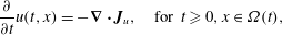
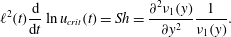
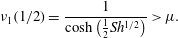
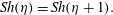
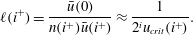
Figure 1 is a 1D illustration of the advancement $\text{d}s$
of the ice–water boundary over an infinitesimal time
$\text{d}s$
of the ice–water boundary over an infinitesimal time $\text{d}t$
, due to the increase of the critical salinity at the boundary from
$\text{d}t$
, due to the increase of the critical salinity at the boundary from $u_{crit}$
to
$u_{crit}$
to $u_{crit}+\text{d}u_{crit}$
. This results in the salt-expulsion flux
$u_{crit}+\text{d}u_{crit}$
. This results in the salt-expulsion flux $J_{bc}$
at the boundary and the corresponding change in the overall salt profile from solid to dashed line as a result of the diffusion in the water domain.
$J_{bc}$
at the boundary and the corresponding change in the overall salt profile from solid to dashed line as a result of the diffusion in the water domain.
Figure 1. A sketch of the ice–water boundary movement caused by an increase of the critical salinity during freezing.
2.3 Nucleation
Salinity and phase transition are two processes that are strongly connected. As seen from the discussion above, a decrease in the temperature can lead to freezing associated with existing ice regions through an increase of the critical salinity $u_{crit}$
. A second important mechanism is the nucleation of new ice regions. The exact laws of nucleation are difficult to obtain. We expect supercooling to occur in the system that would trigger the nucleation process when below a (salinity dependent) nucleation temperature. Conversely, it can be stated that nucleation only happens below a (temperature dependent) nucleation salinity. To be consistent with the treatment of freezing, we adopt this latter viewpoint and thus we write
$u_{crit}$
. A second important mechanism is the nucleation of new ice regions. The exact laws of nucleation are difficult to obtain. We expect supercooling to occur in the system that would trigger the nucleation process when below a (salinity dependent) nucleation temperature. Conversely, it can be stated that nucleation only happens below a (temperature dependent) nucleation salinity. To be consistent with the treatment of freezing, we adopt this latter viewpoint and thus we write $u_{nucl}=u_{nucl}(T(t))=u_{nucl}(t)$
. This allows us to naturally define a dimensionless number associated with nucleation,
$u_{nucl}=u_{nucl}(T(t))=u_{nucl}(t)$
. This allows us to naturally define a dimensionless number associated with nucleation,
 $$\begin{eqnarray}\unicode[STIX]{x1D707}(t)=\frac{u_{nucl}(t)}{u_{crit}(t)},\end{eqnarray}$$
where $0\leqslant \unicode[STIX]{x1D707}<1$
has the interpretation of a nucleation multiplier. Once nucleation is encountered, salinity decreases locally due to ice formation (as discussed above), and a measurable region of ice is formed at nucleation sites.
$0\leqslant \unicode[STIX]{x1D707}<1$
has the interpretation of a nucleation multiplier. Once nucleation is encountered, salinity decreases locally due to ice formation (as discussed above), and a measurable region of ice is formed at nucleation sites.
In general, the nucleation multiplier $\unicode[STIX]{x1D707}$
may vary with salinity. For the mathematical analysis in the next section, it is convenient to consider the lowest-order approximation of a constant multiplier. The nucleation multiplier
$\unicode[STIX]{x1D707}$
may vary with salinity. For the mathematical analysis in the next section, it is convenient to consider the lowest-order approximation of a constant multiplier. The nucleation multiplier $\unicode[STIX]{x1D707}$
can also be interpreted as a dimensionless parameter related to the degree of super-saturation of micro-crystals permitted in the fluid for the current salinity, and is thus related to the free energy released for a nucleation event. The interpretation of a constant nucleation multiplier
$\unicode[STIX]{x1D707}$
can also be interpreted as a dimensionless parameter related to the degree of super-saturation of micro-crystals permitted in the fluid for the current salinity, and is thus related to the free energy released for a nucleation event. The interpretation of a constant nucleation multiplier $\unicode[STIX]{x1D707}$
is thus in principle an approximation of a nucleation probability dependent on the deviation in free energy from the equilibrium state (Mullin Reference Mullin2001). One should note that the first-order approximation of (2.9) around the regime of interest might not be extended to arbitrary values of concentration; our model for instance does not capture undercooling of freshwater.
$\unicode[STIX]{x1D707}$
is thus in principle an approximation of a nucleation probability dependent on the deviation in free energy from the equilibrium state (Mullin Reference Mullin2001). One should note that the first-order approximation of (2.9) around the regime of interest might not be extended to arbitrary values of concentration; our model for instance does not capture undercooling of freshwater.
2.4 The complete mathematical model
In the continuation, we will always consider the space, the time and the concentration dimensionless. More precisely, we use the natural non-dimensionalizations $x/x_{\ast }\rightarrow x$
,
$x/x_{\ast }\rightarrow x$
, $u_{crit}(t)/u_{crit}(0)\rightarrow u_{crit}(t)$
and
$u_{crit}(t)/u_{crit}(0)\rightarrow u_{crit}(t)$
and $t/t_{\ast }\rightarrow t$
where
$t/t_{\ast }\rightarrow t$
where $t_{\ast }=(x_{\ast })^{2}/D$
. Here
$t_{\ast }=(x_{\ast })^{2}/D$
. Here $x_{\ast }$
is the diameter of the domain (length, in 1D) and
$x_{\ast }$
is the diameter of the domain (length, in 1D) and $t_{\ast }$
a characteristic time. By this, the non-dimensionalized
$t_{\ast }$
a characteristic time. By this, the non-dimensionalized $u_{crit}(0)=1$
and the dimensionless diffusion coefficient becomes 1.
$u_{crit}(0)=1$
and the dimensionless diffusion coefficient becomes 1.
The mathematical model discussed so far has the salinity $u$
and the location of the ice–brine boundary
$u$
and the location of the ice–brine boundary $\unicode[STIX]{x2202}\unicode[STIX]{x1D6FA}$
as unknowns. The process is governed by the critical salinity at the ice–brine interface
$\unicode[STIX]{x2202}\unicode[STIX]{x1D6FA}$
as unknowns. The process is governed by the critical salinity at the ice–brine interface $u_{crit}$
, which is temperature and thus time dependent and defines the boundary conditions at
$u_{crit}$
, which is temperature and thus time dependent and defines the boundary conditions at $\unicode[STIX]{x2202}\unicode[STIX]{x1D6FA}(t)$
.
$\unicode[STIX]{x2202}\unicode[STIX]{x1D6FA}(t)$
.
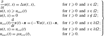 $$\begin{eqnarray}\left.\begin{array}{@{}ll@{}}\displaystyle \frac{\unicode[STIX]{x2202}}{\unicode[STIX]{x2202}t}u(t,x)=\unicode[STIX]{x0394}u(t,x), & \text{for }t\geqslant 0\text{ and }x\in \unicode[STIX]{x1D6FA};\\ u(t,x)\geqslant u_{nucl}(t) & \text{for }t\geqslant 0\text{ and }x\in \unicode[STIX]{x1D6FA};\\ u(t,x)=0 & \text{for }t\geqslant 0\text{ and }x\notin \unicode[STIX]{x1D6FA};\\ \displaystyle u_{crit}(t)\frac{\text{d}}{\text{d}t}\boldsymbol{s}(t)\boldsymbol{\cdot }\boldsymbol{n}=(-\unicode[STIX]{x1D735}u(t,x))\boldsymbol{\cdot }\boldsymbol{n}, & \text{for }t\geqslant 0\text{ and }x\in \unicode[STIX]{x2202}\unicode[STIX]{x1D6FA};\\ u(t,x)=u_{crit}(t) & \text{for }t\geqslant 0\text{ and }x\in \unicode[STIX]{x2202}\unicode[STIX]{x1D6FA};\\ u_{nucl}(t)=\unicode[STIX]{x1D707}u_{crit}(t), & \text{for }t\geqslant 0.\end{array}\right\}\end{eqnarray}$$
The system is completed by initial conditions.
2.5 Sherwood number
In the absence of spontaneous nucleation, the qualitative behaviour of the ice–water system can be characterized by a relation between the rate of the normal components of two fluxes at the moving ice–brine boundary: the salt-expulsion flux (2.7) and the diffusive flux (2.4). We let $\ell$
be a time-dependent characteristic domain size that can be seen as an average distance between ice boundaries. Observe that the entire process considered here is controlled by the critical salinity
$\ell$
be a time-dependent characteristic domain size that can be seen as an average distance between ice boundaries. Observe that the entire process considered here is controlled by the critical salinity $u_{crit}$
and this can change rapidly in time, inducing different ice-formation regimes. Consequently, the characteristic domain size
$u_{crit}$
and this can change rapidly in time, inducing different ice-formation regimes. Consequently, the characteristic domain size $\ell$
may change significantly in time.
$\ell$
may change significantly in time.
We interpret $K$
as a characteristic normal velocity of the ice–brine boundary (to be defined precisely below), which scales as
$K$
as a characteristic normal velocity of the ice–brine boundary (to be defined precisely below), which scales as
 $$\begin{eqnarray}K\sim \frac{\text{d}\boldsymbol{s}}{\text{d}t}\boldsymbol{\cdot }\boldsymbol{n}.\end{eqnarray}$$
The ratio of mass-transfer rate to the diffusion rate is essential for this problem and is characterized by the Sherwood number (Cussler Reference Cussler2009), defined as (recall that the non-dimensionalized diffusion constant is unity)
 $$\begin{eqnarray}Sh=\frac{K}{\ell ^{-1}}.\end{eqnarray}$$
We emphasize that $Sh$
may change in time as it depends on both
$Sh$
may change in time as it depends on both $\ell$
and
$\ell$
and $K$
, thus it is in principle a function. By a slight abuse of language, we will nevertheless refer to
$K$
, thus it is in principle a function. By a slight abuse of language, we will nevertheless refer to $Sh$
as a ‘number’. The case where
$Sh$
as a ‘number’. The case where $Sh$
is constant in time will be of particular importance later.
$Sh$
is constant in time will be of particular importance later.
To make concrete the choice of $K$
, recall that the evolution of the ice–water interface is not known a priori but represents an unknown in the model. This evolution is controlled by
$K$
, recall that the evolution of the ice–water interface is not known a priori but represents an unknown in the model. This evolution is controlled by $u_{crit}$
, which is a time-dependent input parameter of the model. As mentioned,
$u_{crit}$
, which is a time-dependent input parameter of the model. As mentioned, $K$
itself depends on time through
$K$
itself depends on time through $\ell$
, which in its turn depends on
$\ell$
, which in its turn depends on $u_{crit}$
. Therefore it makes sense to express
$u_{crit}$
. Therefore it makes sense to express $K$
in terms of critical salinity. To do so we first refer to figure 1 sketching the change in the ice–brine system encountered within an infinitesimal time
$K$
in terms of critical salinity. To do so we first refer to figure 1 sketching the change in the ice–brine system encountered within an infinitesimal time $\text{d}t$
. More precisely, as suggested by the area of fresh ice, in the normal direction the ice front is moving into the brine over the infinitesimal distance
$\text{d}t$
. More precisely, as suggested by the area of fresh ice, in the normal direction the ice front is moving into the brine over the infinitesimal distance $\text{d}\boldsymbol{s}\boldsymbol{\cdot }\boldsymbol{n}$
, causing salt expulsion into the brine. The corresponding normal salt flux
$\text{d}\boldsymbol{s}\boldsymbol{\cdot }\boldsymbol{n}$
, causing salt expulsion into the brine. The corresponding normal salt flux $\boldsymbol{J}_{bc}\boldsymbol{\cdot }\boldsymbol{n}\,\text{d}t$
can be obtained from (2.7). Consequently, the salt is distributed into the brine domain sized
$\boldsymbol{J}_{bc}\boldsymbol{\cdot }\boldsymbol{n}\,\text{d}t$
can be obtained from (2.7). Consequently, the salt is distributed into the brine domain sized $\ell$
(the left part of 1), causing an increase in the salinity by
$\ell$
(the left part of 1), causing an increase in the salinity by $\text{d}\,u_{crit}$
(the grey dashed curve). By mass conservation, one gets
$\text{d}\,u_{crit}$
(the grey dashed curve). By mass conservation, one gets
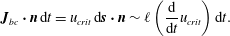 $$\begin{eqnarray}\boldsymbol{J}_{bc}\boldsymbol{\cdot }\boldsymbol{n}\,\text{d}t=u_{crit}\,\text{d}\boldsymbol{s}\boldsymbol{\cdot }\boldsymbol{n}\sim \ell \left(\frac{\text{d}}{\text{d}t}u_{crit}\right)\text{d}t.\end{eqnarray}$$
Dividing in the above by $u_{crit}\,\text{d}t$
, from (2.11) we obtain the definition of the characteristic velocity of the system
$u_{crit}\,\text{d}t$
, from (2.11) we obtain the definition of the characteristic velocity of the system
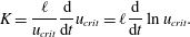 $$\begin{eqnarray}\displaystyle K=\frac{\ell }{u_{crit}}\frac{\text{d}}{\text{d}t}u_{crit}=\ell \frac{\text{d}}{\text{d}t}\ln u_{crit}. & & \displaystyle\end{eqnarray}$$
Combining the definition of the characteristic normal velocity with the Sherwood number in (2.12), we obtain
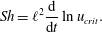 $$\begin{eqnarray}Sh=\ell ^{2}\frac{\text{d}}{\text{d}t}\ln u_{crit}.\end{eqnarray}$$
The Sherwood number as defined above will play a critical role in our subsequent analysis.
In addition to the Sherwood number, the model under discussion is also influenced by the nucleation threshold. This is accounted for through the nucleation multiplier $\unicode[STIX]{x1D707}$
defined by equation (2.9), which is already a dimensionless parameter. In § 4 we show that the qualitative behaviour of the system can be characterized based exclusively on two dimensionless parameters: the Sherwood number
$\unicode[STIX]{x1D707}$
defined by equation (2.9), which is already a dimensionless parameter. In § 4 we show that the qualitative behaviour of the system can be characterized based exclusively on two dimensionless parameters: the Sherwood number $Sh$
and the nucleation multiplier
$Sh$
and the nucleation multiplier $\unicode[STIX]{x1D707}$
.
$\unicode[STIX]{x1D707}$
.
2.6 The dimensionless variables in 1D
While the mathematical model defined above is stated for arbitrary dimensions, the analysis in the remainder of this manuscript is restricted to the case of one spatial dimension. For concreteness, we reformulate the variables of (2.10) accordingly, by employing the characteristic quantities discussed in § 2.5.
Since in 1D the brine domain is a union of sub-intervals, we fix $t>0$
and for any brine interval we let
$t>0$
and for any brine interval we let $x_{0}(t)$
denote its left boundary and
$x_{0}(t)$
denote its left boundary and $\ell (t)$
its length. This allows us to rescale the spatial coordinate
$\ell (t)$
its length. This allows us to rescale the spatial coordinate $x$
and introduce a local coordinate
$x$
and introduce a local coordinate $y$
on each brine interval
$y$
on each brine interval
 $$\begin{eqnarray}y=(x-x_{0}(t))/\ell (t).\end{eqnarray}$$
In this way, for each sub-interval of brine the solution is defined on the unit interval $y\in [0,1]$
.
$y\in [0,1]$
.
Now note that the freezing and nucleation given in (2.10) ensures that for the salinity $u$
, one has
$u$
, one has
 $$\begin{eqnarray}\displaystyle \unicode[STIX]{x1D707}u_{crit}(t)<u\leqslant u_{crit}(t), & & \displaystyle\end{eqnarray}$$
for any $t>0$
and
$t>0$
and $x$
in the brine domain. It therefore makes sense to introduce a time-dependent normalization by the salinity
$x$
in the brine domain. It therefore makes sense to introduce a time-dependent normalization by the salinity $u_{crit}$
, such that the dimensionless salinity is constrained to the time-independent interval
$u_{crit}$
, such that the dimensionless salinity is constrained to the time-independent interval $(\unicode[STIX]{x1D707},1]$
. This allows us to define a dimensionless salinity
$(\unicode[STIX]{x1D707},1]$
. This allows us to define a dimensionless salinity $\unicode[STIX]{x1D708}$
for a sub-domain through
$\unicode[STIX]{x1D708}$
for a sub-domain through
 $$\begin{eqnarray}\unicode[STIX]{x1D708}:(0,\infty )\times (0,1)\rightarrow (\unicode[STIX]{x1D707},1],\quad \unicode[STIX]{x1D708}(t,y)=\unicode[STIX]{x1D708}(t,(x-x_{0}(t))/\ell (t))=\frac{u(t,x)}{u_{crit}(t)}.\end{eqnarray}$$
Note that the time is dimensionless, as rescaled in § 2.4. Also, since in the dimensionless form $y=0$
and
$y=0$
and $y=1$
are ice–brine boundaries and due to the scaling of the salinity one has
$y=1$
are ice–brine boundaries and due to the scaling of the salinity one has $\unicode[STIX]{x1D708}(0)=\unicode[STIX]{x1D708}(1)=1$
. By (2.9),
$\unicode[STIX]{x1D708}(0)=\unicode[STIX]{x1D708}(1)=1$
. By (2.9), $\unicode[STIX]{x1D708}$
cannot decrease below
$\unicode[STIX]{x1D708}$
cannot decrease below $\unicode[STIX]{x1D707}$
. In other words, whenever the minimum of
$\unicode[STIX]{x1D707}$
. In other words, whenever the minimum of $\unicode[STIX]{x1D708}$
is close to
$\unicode[STIX]{x1D708}$
is close to $\unicode[STIX]{x1D707}$
, the system is close to nucleation.
$\unicode[STIX]{x1D707}$
, the system is close to nucleation.
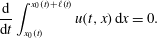
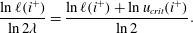
3 Rapid freezing in 1D
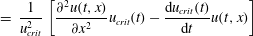
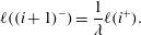
Figure 2. Salinity evolution in the fluid domain during rapid freezing (darker plots correspond to more recent times).
In the simplified 1D setting we consider, brine occupies the non-dimensional interval $\unicode[STIX]{x1D6FA}(0)\equiv (0,1)$
, and (without loss of generality) we assume that ice is present at both boundaries. This can be the result of an initial nucleation.
$\unicode[STIX]{x1D6FA}(0)\equiv (0,1)$
, and (without loss of generality) we assume that ice is present at both boundaries. This can be the result of an initial nucleation.
The evolution of the salinity in a brine interval during rapid freezing is illustrated in figure 2, where three typical salinity profiles are displayed. To be more precise, if the environmental temperature is decreasing, the ice front advances into the brine. As stated, the temperature decrease is associated with an increase in the critical salinity, as given in equation (2.2). This process can be observed in figure 2, where the brine domain is shrinking with time. On the other hand, the diffusion smoothes out the oscillations and propagates the increase in the salinity at the boundary towards the centre of the fluid domain.
In the first instance, if the freezing is rapid the salinity changes near the boundary are larger than the changes in the interior. This leads to salinity profiles taking maximal values equal to $u_{crit}$
at the domain boundaries (the ice–brine interface) and lower ones in the middle of the fluid domain (see figure 2). In fact, the diffusion and the temperature decrease (or the increase of
$u_{crit}$
at the domain boundaries (the ice–brine interface) and lower ones in the middle of the fluid domain (see figure 2). In fact, the diffusion and the temperature decrease (or the increase of $u_{crit}$
) are two effects that determine the behaviour of the system. Their interplay is characterized by the Sherwood number
$u_{crit}$
) are two effects that determine the behaviour of the system. Their interplay is characterized by the Sherwood number $Sh$
discussed in § 2.5. In this context, three regimes can be identified, ordered by increasing Sherwood numbers:
$Sh$
discussed in § 2.5. In this context, three regimes can be identified, ordered by increasing Sherwood numbers:
-
(i) the sub-critical regime, when diffusion dominates and the solubility profiles are flattened out to $u_{crit}$
to form a continuous ice;
$u_{crit}$
to form a continuous ice; -
(ii) the critical regime, when diffusion balances the salinity changes due to temperature decrease, leading to self-similar solutions;
-
(iii) the super-critical regime, when the temperature decrease dominates. In this case, the ratio between the minimum and the maximum values of the solubilities decreases until it reaches the nucleation multiplier defined in (2.9). At that point the domain is split in two and the process continues in each sub-domain. If this process continues infinitely it will result in a Cantor-like set of sub-domains.

Since the Sherwood number is in principle changing in time, the system can switch from sub-critical to super-critical regimes and vice versa. The critical regime is the transition between the two regimes of compact and fractal ice growth. The reminder of this section is devoted to derivation of the specific temporal controls of $u_{crit}$
which result in the critical and super-critical regimes.
$u_{crit}$
which result in the critical and super-critical regimes.
3.1 The critical case
We define the critical case to be the state where the salinity profile is self-similar and thus represents a case where no nucleation events occur. In other words, diffusion is in balance with the temperature decrease, representing a bifurcation point for the system. Recall that the dimensionless solution function $\unicode[STIX]{x1D708}$
, as defined in (2.18), is in this case constant in time
$\unicode[STIX]{x1D708}$
, as defined in (2.18), is in this case constant in time
 $$\begin{eqnarray}\frac{\unicode[STIX]{x2202}\unicode[STIX]{x1D708}(t,y)}{\unicode[STIX]{x2202}t}=0.\end{eqnarray}$$
To simplify the notation, since $\unicode[STIX]{x1D708}$
does not depend on time, we will in this section use the notation
$\unicode[STIX]{x1D708}$
does not depend on time, we will in this section use the notation
 $$\begin{eqnarray}\unicode[STIX]{x1D708}_{1}(y)\equiv \unicode[STIX]{x1D708}(t,y).\end{eqnarray}$$
To find the boundary conditions leading to the critical case we consider $\unicode[STIX]{x1D708}_{1}$
as a self-similar solution of the original problem, in the spirit of Barenblatt (Reference Barenblatt1996). Using (2.16) and (2.5) together with the chain rule, we obtain
$\unicode[STIX]{x1D708}_{1}$
as a self-similar solution of the original problem, in the spirit of Barenblatt (Reference Barenblatt1996). Using (2.16) and (2.5) together with the chain rule, we obtain
 $$\begin{eqnarray}\displaystyle 0=\frac{\unicode[STIX]{x2202}\unicode[STIX]{x1D708}_{1}(y)}{\unicode[STIX]{x2202}t}\equiv \frac{\unicode[STIX]{x2202}\unicode[STIX]{x1D708}(t,y)}{\unicode[STIX]{x2202}t} & = & \displaystyle \frac{1}{u_{crit}^{2}}\left[\frac{\unicode[STIX]{x2202}u(t,x)}{\unicode[STIX]{x2202}t}u_{crit}-\frac{\text{d}u_{crit}(t)}{\text{d}t}u\right]\end{eqnarray}$$
 $$\begin{eqnarray}\displaystyle & = & \displaystyle \frac{1}{u_{crit}^{2}}\left[\frac{\unicode[STIX]{x2202}^{2}u(t,x)}{\unicode[STIX]{x2202}x^{2}}u_{crit}(t)-\frac{\text{d}u_{crit}(t)}{\text{d}t}u(t,x)\right]\end{eqnarray}$$
 $$\begin{eqnarray}\displaystyle & = & \displaystyle \frac{1}{\ell ^{2}(t)}\frac{\unicode[STIX]{x2202}^{2}\unicode[STIX]{x1D708}_{1}(y)}{\unicode[STIX]{x2202}y^{2}}-\frac{1}{u_{crit}(t)}\frac{\text{d}u_{crit}(t)}{\text{d}t}\unicode[STIX]{x1D708}_{1}(y).\end{eqnarray}$$
This expression, together with the definition of the Sherwood number given in equation (2.15) provides an equation for the self-similar solution $\unicode[STIX]{x1D708}_{1}$
 $$\begin{eqnarray}\ell ^{2}(t)\frac{\text{d}}{\text{d}t}\ln u_{crit}(t)=Sh=\frac{\unicode[STIX]{x2202}^{2}\unicode[STIX]{x1D708}_{1}(y)}{\unicode[STIX]{x2202}y^{2}}\frac{1}{\unicode[STIX]{x1D708}_{1}(y)}.\end{eqnarray}$$
Since the self-similar solution $\unicode[STIX]{x1D708}_{1}$
does not include an explicit time dependency, we make the essential observation that for the critical case the Sherwood number is constant. Thus equation (3.6) provides two results. First, it is an ordinary differential equation for the boundary salinity
$\unicode[STIX]{x1D708}_{1}$
does not include an explicit time dependency, we make the essential observation that for the critical case the Sherwood number is constant. Thus equation (3.6) provides two results. First, it is an ordinary differential equation for the boundary salinity $u_{crit}$
leading to a constant Sherwood number. Second, it is an equation providing the self-similar solution
$u_{crit}$
leading to a constant Sherwood number. Second, it is an equation providing the self-similar solution $\unicode[STIX]{x1D708}_{1}$
for this external control.
$\unicode[STIX]{x1D708}_{1}$
for this external control.
3.1.1 The external control required for the critical case
We start with interpreting equation (3.6) in terms of $u_{crit}$
. Observe that it involves two unknowns,
$u_{crit}$
. Observe that it involves two unknowns, $u_{crit}$
and
$u_{crit}$
and $\ell$
. These unknowns are related by mass conservation of salt in the whole fluid domain, as there are no nucleation events.
$\ell$
. These unknowns are related by mass conservation of salt in the whole fluid domain, as there are no nucleation events.
In other words, mass conservation for salt gives us in terms of non-scaled variables
 $$\begin{eqnarray}\frac{\text{d}}{\text{d}t}\int _{x_{0}(t)}^{x_{0}(t)+\ell (t)}u(t,x)\,\text{d}x=0.\end{eqnarray}$$
Using the definition of $\unicode[STIX]{x1D708}_{1}$
and transforming the above to the domain
$\unicode[STIX]{x1D708}_{1}$
and transforming the above to the domain $[0,1]$
yields
$[0,1]$
yields
 $$\begin{eqnarray}\frac{\text{d}}{\text{d}t}\left[\ell (t)u_{crit}(t)\int _{0}^{1}\unicode[STIX]{x1D708}_{1}(y)\,\text{d}y\right]=0.\end{eqnarray}$$
Since the integral is independent of time, we can conclude that the product of domain size and critical concentration is independent of time, i.e.
 $$\begin{eqnarray}\ell (t)u_{crit}(t)=u_{crit,0}\ell =1.\end{eqnarray}$$
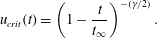
Combining equations (3.6) and (3.9) we obtain
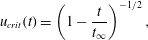 $$\begin{eqnarray}u_{crit}(t)=\left(1-\frac{t}{t_{\infty }}\right)^{-1/2},\end{eqnarray}$$
where the integration constant is identified as the time before the brine salinity blows up, which is related to the Sherwood number by
 $$\begin{eqnarray}t_{\infty }=\frac{1}{2Sh}.\end{eqnarray}$$
We note that from equations (3.9) and (3.11) that the size of the brine region satisfies $\ell (t)=(1-t/t_{\infty })^{1/2}$
. Thus consistent with the notion of mass conservation, as the salinity blows up when
$\ell (t)=(1-t/t_{\infty })^{1/2}$
. Thus consistent with the notion of mass conservation, as the salinity blows up when $t$
approaches
$t$
approaches $t_{\infty }$
, the brine domain vanishes,
$t_{\infty }$
, the brine domain vanishes, $\ell (t_{\infty })=0$
.
$\ell (t_{\infty })=0$
.
3.1.2 The salinity in the critical case
We now solve equation (3.6) to obtain $\unicode[STIX]{x1D708}_{1}$
and from this we find the salinity. From the definition of
$\unicode[STIX]{x1D708}_{1}$
and from this we find the salinity. From the definition of $\unicode[STIX]{x1D708}$
in (2.18) the boundary conditions are
$\unicode[STIX]{x1D708}$
in (2.18) the boundary conditions are
 $$\begin{eqnarray}\unicode[STIX]{x1D708}_{1}(0)=\unicode[STIX]{x1D708}_{1}(1)=1.\end{eqnarray}$$
The solution to (3.6) satisfying these conditions is
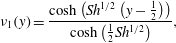 $$\begin{eqnarray}\unicode[STIX]{x1D708}_{1}(y)=\frac{\cosh \left(Sh^{1/2}\left(y-\frac{1}{2}\right)\right)}{\cosh \left(\frac{1}{2}Sh^{1/2}\right)},\end{eqnarray}$$
where $\cosh$
is the hyperbolic cosine function. Equation (3.13) defines a family of solutions depending on the Sherwood number.
$\cosh$
is the hyperbolic cosine function. Equation (3.13) defines a family of solutions depending on the Sherwood number.
The above solutions are obtained in the absence of nucleation, in the sense that the constraint $\unicode[STIX]{x1D708}\geqslant \unicode[STIX]{x1D707}$
has not been enforced. The self-similar solution
$\unicode[STIX]{x1D708}\geqslant \unicode[STIX]{x1D707}$
has not been enforced. The self-similar solution $\unicode[STIX]{x1D708}_{1}$
has a minimum at
$\unicode[STIX]{x1D708}_{1}$
has a minimum at $y=1/2$
, thus the nucleation threshold is given as
$y=1/2$
, thus the nucleation threshold is given as
 $$\begin{eqnarray}\unicode[STIX]{x1D708}_{1}(1/2)=\frac{1}{\cosh \left(\frac{1}{2}Sh^{1/2}\right)}>\unicode[STIX]{x1D707}.\end{eqnarray}$$
Since the self-similar solution is not valid across nucleation events, we interpret inequality (3.14) as a constraint on admissible Sherwood numbers for the critical solution, i.e. the freezing must be sufficiently slow such that
 $$\begin{eqnarray}Sh\leqslant \left(2\text{arcCosh}\frac{1}{\unicode[STIX]{x1D707}}\right)^{2}.\end{eqnarray}$$
This bound on the Sherwood number is essential, as it defines the largest possible constant Sherwood number for this system. When inequality (3.15) is violated over an extended time period, i.e. for a constant Sherwood number, nucleation will happen, and thus the length scale $\ell$
will be reduced, thus also reducing the Sherwood number. Conversely, we can consider the equality (3.15) as a characteristic property of nucleation events. We explore these concepts in § 4.
$\ell$
will be reduced, thus also reducing the Sherwood number. Conversely, we can consider the equality (3.15) as a characteristic property of nucleation events. We explore these concepts in § 4.
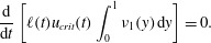
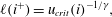
3.2 A super-critical, fractal case
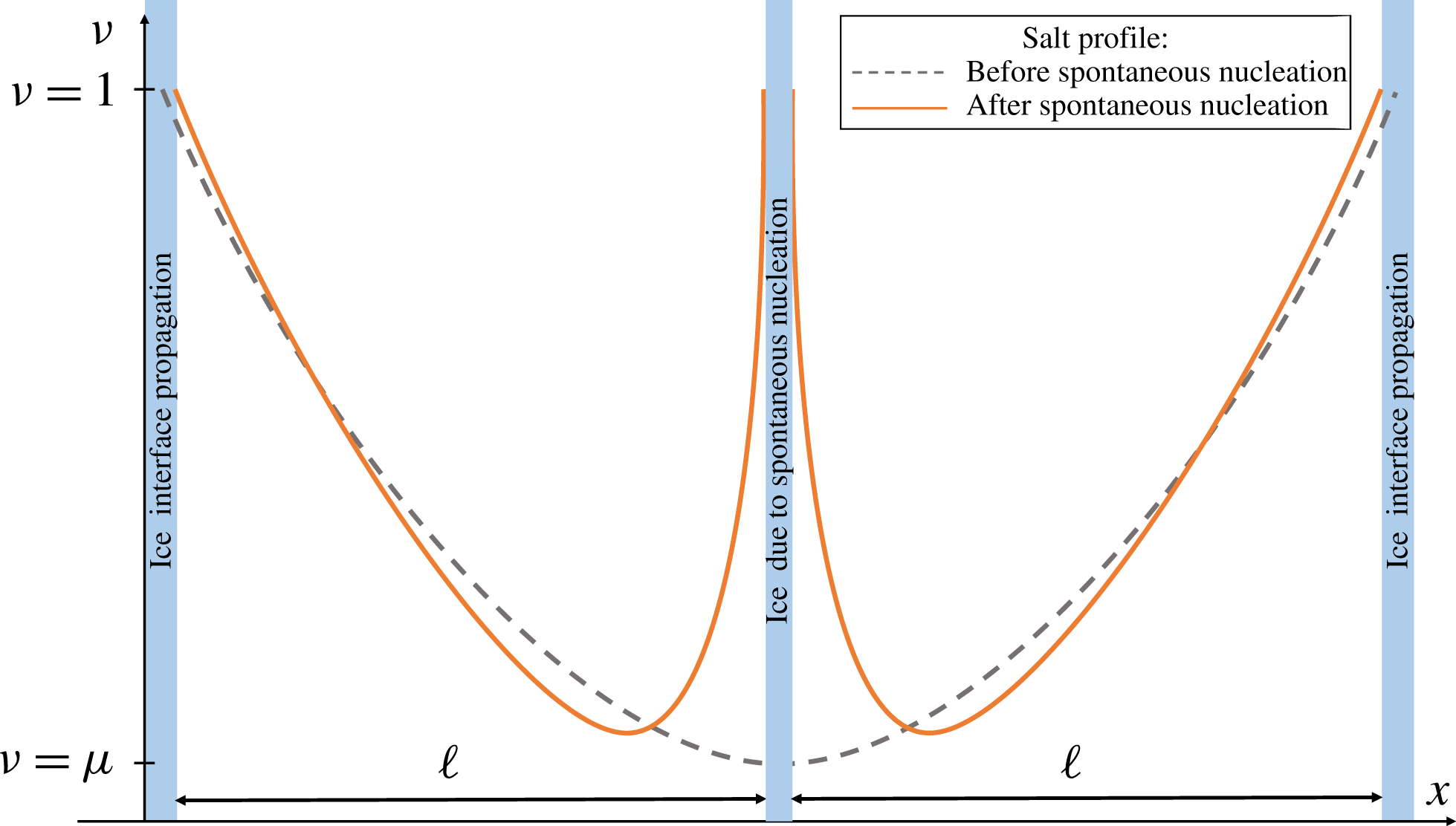
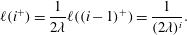
Figure 3. A schematic plot illustrating the change in the solution $u$
due to spontaneous nucleation in the middle of the domain.
$u$
due to spontaneous nucleation in the middle of the domain.
Super-critical freezing appears when cooling dominates diffusion. Due to this, an increase of the critical salinity is encountered and $\unicode[STIX]{x1D708}$
, the ratio between the critical salinity and the minimal one, decreases until it reaches
$\unicode[STIX]{x1D708}$
, the ratio between the critical salinity and the minimal one, decreases until it reaches $\unicode[STIX]{x1D707}$
, at which time nucleation occurs. For symmetry reasons we expect that nucleation happens near the middle of a brine domain, we approximate the splitting of the domain into two equal parts – see figure 3. This leads to two domains of halved lengths and, by (2.15), to a decrease in the Sherwood number. A lower Sherwood number together with a steeper salinity gradient near the newly created boundaries lead to a local diffusion-dominated solution profile until freezing starts to dominate again and the process repeats itself. The period where the solution is diffusion dominated is essential in order to transition from a non-symmetric profile after a nucleation event (solid line, figure 3), towards an asymptotically symmetric profile before the next nucleation event happens. Following this scenario, one may expect a fractal structure similar to a Cantor set for the fluid domain.
$\unicode[STIX]{x1D707}$
, at which time nucleation occurs. For symmetry reasons we expect that nucleation happens near the middle of a brine domain, we approximate the splitting of the domain into two equal parts – see figure 3. This leads to two domains of halved lengths and, by (2.15), to a decrease in the Sherwood number. A lower Sherwood number together with a steeper salinity gradient near the newly created boundaries lead to a local diffusion-dominated solution profile until freezing starts to dominate again and the process repeats itself. The period where the solution is diffusion dominated is essential in order to transition from a non-symmetric profile after a nucleation event (solid line, figure 3), towards an asymptotically symmetric profile before the next nucleation event happens. Following this scenario, one may expect a fractal structure similar to a Cantor set for the fluid domain.
In the spirit of the critical case described in § 3.1 we seek a self-similar solution in the super-critical case, which will provide insight as to the structures arising during rapid freezing. However, in this case nucleation, and hence brine interval splitting, is encountered at certain times, which is the underlying mechanism for generating fractal solutions. Since $\ell$
is discontinuous in time we understand that, unlike the critical case, we cannot have a constant Sherwood number and thus a freezing-rate scaling (3.10) will not work. Indeed, in this section, we will show that for an external control of the critical salinity which is strictly faster than (3.10), persistent nucleation can occur. The explicit solution derived herein thus provides a connection between the external control on the critical salinity and the relative freezing and nucleation processes.
$\ell$
is discontinuous in time we understand that, unlike the critical case, we cannot have a constant Sherwood number and thus a freezing-rate scaling (3.10) will not work. Indeed, in this section, we will show that for an external control of the critical salinity which is strictly faster than (3.10), persistent nucleation can occur. The explicit solution derived herein thus provides a connection between the external control on the critical salinity and the relative freezing and nucleation processes.
As the domain splits into smaller sub-domains, the typical length scale becomes smaller and the same should happen with the time scale characterizing the process between two nucleation events. To reflect this, a nonlinear transformation of the time variable is introduced, with respect to which the dimensionless solution $\unicode[STIX]{x1D708}$
has a periodic behaviour
$\unicode[STIX]{x1D708}$
has a periodic behaviour
 $$\begin{eqnarray}t=f(\unicode[STIX]{x1D702}).\end{eqnarray}$$
The function $f$
is a nonlinear, continuous and increasing transformation of time, which will be specified later. At present we require that the transformation ensures that
$f$
is a nonlinear, continuous and increasing transformation of time, which will be specified later. At present we require that the transformation ensures that $\unicode[STIX]{x1D708}$
is periodic with period 1 in the transformed time variable
$\unicode[STIX]{x1D708}$
is periodic with period 1 in the transformed time variable $\unicode[STIX]{x1D702}$
.
$\unicode[STIX]{x1D702}$
.
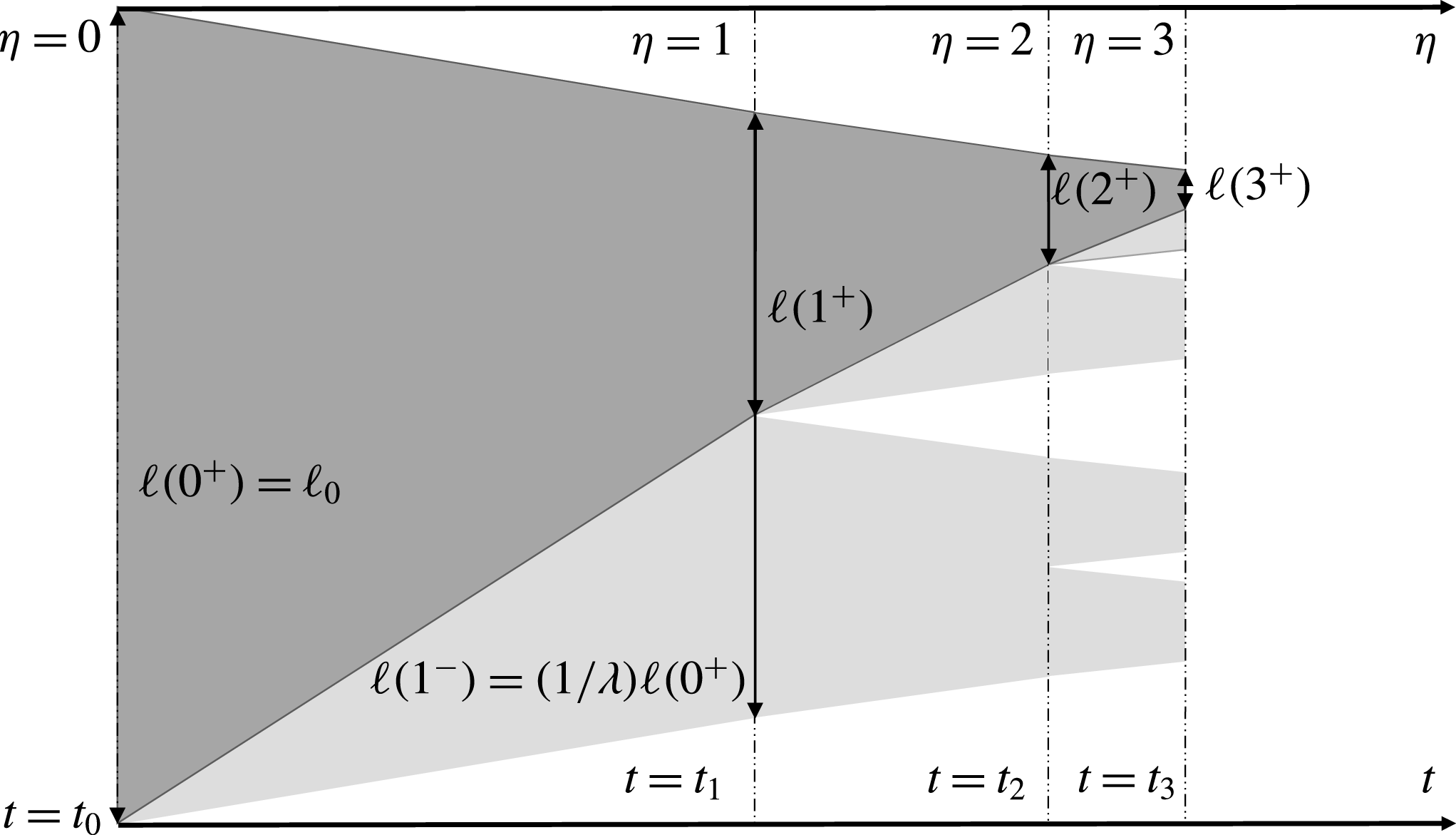
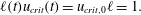
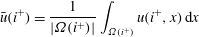
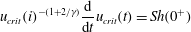
Figure 4. A conceptual illustration of the changes in the brine domain size during fractal-forming freezing. Regions of brine are represented as grey, with the darker overlay representing the smoothed, $\unicode[STIX]{x1D702}$
-independent approximation of a continuous brine sub-domain size evolving through time.
$\unicode[STIX]{x1D702}$
-independent approximation of a continuous brine sub-domain size evolving through time.
In the critical case discussed in § 3.1 the Sherwood number was constant in time. Here we use the ansatz that the Sherwood number has the same periodic structure as the domain, i.e. that it is one-periodic with respect to the time variable $\unicode[STIX]{x1D702}$
:
$\unicode[STIX]{x1D702}$
:
 $$\begin{eqnarray}Sh(\unicode[STIX]{x1D702})=Sh(\unicode[STIX]{x1D702}+1).\end{eqnarray}$$
In the super-critical case the brine domain $\unicode[STIX]{x1D6FA}$
is complex, consisting of several sub-domains (intervals). Since the Sherwood number is no longer constant in the nucleation case, we introduce a new parameter to characterize the system in this regime. Thus let
$\unicode[STIX]{x1D6FA}$
is complex, consisting of several sub-domains (intervals). Since the Sherwood number is no longer constant in the nucleation case, we introduce a new parameter to characterize the system in this regime. Thus let $\unicode[STIX]{x1D706}>1$
be a similarity parameter, such that between two nucleation events each interval decreases
$\unicode[STIX]{x1D706}>1$
be a similarity parameter, such that between two nucleation events each interval decreases $\unicode[STIX]{x1D706}$
times as the ice boundaries propagate inwards. This non-dimensionless parameter thus gives the balance between freezing and nucleation. In particular, small values of
$\unicode[STIX]{x1D706}$
times as the ice boundaries propagate inwards. This non-dimensionless parameter thus gives the balance between freezing and nucleation. In particular, small values of $\unicode[STIX]{x1D706}$
close to
$\unicode[STIX]{x1D706}$
close to $1$
represent nucleation-dominated regimes, while large values of
$1$
represent nucleation-dominated regimes, while large values of $\unicode[STIX]{x1D706}$
represent freezing-dominated regimes.
$\unicode[STIX]{x1D706}$
represent freezing-dominated regimes.
The definition of the time variable $\unicode[STIX]{x1D702}$
is such that nucleation events occur at integer values, which we will denote for clarity by
$\unicode[STIX]{x1D702}$
is such that nucleation events occur at integer values, which we will denote for clarity by $i$
. The definition of the similarity variable
$i$
. The definition of the similarity variable $\unicode[STIX]{x1D706}$
thus implies that
$\unicode[STIX]{x1D706}$
thus implies that
 $$\begin{eqnarray}\ell ((i+1)^{-})=\frac{1}{\unicode[STIX]{x1D706}}\ell (i^{+}).\end{eqnarray}$$
The superscripts $\pm$
should be interpreted as the right and left limits, see figure 4. Further, once a spontaneous nucleation event is encountered in an interval each fluid sub-domain splits into two halves, thus
$\pm$
should be interpreted as the right and left limits, see figure 4. Further, once a spontaneous nucleation event is encountered in an interval each fluid sub-domain splits into two halves, thus $2\ell (i^{+})=\ell (i^{-})$
and the total decrease of the domain over one self-similarity period is given by:
$2\ell (i^{+})=\ell (i^{-})$
and the total decrease of the domain over one self-similarity period is given by:
 $$\begin{eqnarray}\ell (i^{+})=\frac{1}{2\unicode[STIX]{x1D706}}\ell ((i-1)^{+})=\frac{1}{(2\unicode[STIX]{x1D706})^{i}}.\end{eqnarray}$$
Additionally, we can express mass conservation of salt in the system by accounting for the number of brine regions $n(i^{+})$
 $$\begin{eqnarray}n(i^{+})\ell (i^{+})\bar{u}(i^{+})=n(0)\ell (0)\bar{u}(0)=\bar{u}(0),\end{eqnarray}$$
where
 $$\begin{eqnarray}\displaystyle \bar{u}(i^{+})=\frac{1}{|\unicode[STIX]{x1D6FA}(i^{+})|}\int _{\unicode[STIX]{x1D6FA}(i^{+})}u(i^{+},x)\,\text{d}x & & \displaystyle\end{eqnarray}$$
stands for the average salinity in the brine at time $i^{+}$
. The quantity of
$i^{+}$
. The quantity of $\bar{u}(i^{+})$
is unknown but can be approximated by
$\bar{u}(i^{+})$
is unknown but can be approximated by $u_{crit}(i^{+})$
. Combining this with the initial conditions assuming a single brine region of length one allows us to deduce the characteristic domain size
$u_{crit}(i^{+})$
. Combining this with the initial conditions assuming a single brine region of length one allows us to deduce the characteristic domain size
 $$\begin{eqnarray}\ell (i^{+})=\frac{\bar{u}(0)}{n(i^{+})\bar{u}(i^{+})}\approx \frac{1}{2^{i}u_{crit}(i^{+})}.\end{eqnarray}$$
Here we also used that by definition $n(i^{+})=2^{i}$
. Eliminating
$n(i^{+})=2^{i}$
. Eliminating $i$
from equations (3.19) and (3.22) gives
$i$
from equations (3.19) and (3.22) gives
 $$\begin{eqnarray}\frac{\ln \ell (i^{+})}{\ln 2\unicode[STIX]{x1D706}}=\frac{\ln \ell (i^{+})+\ln u_{crit}(i^{+})}{\ln 2}.\end{eqnarray}$$
From equation (3.23) we can now express $\ell$
as an explicit function of
$\ell$
as an explicit function of $u_{crit}$
 $$\begin{eqnarray}\ell (i^{+})=u_{crit}(i)^{-1/\unicode[STIX]{x1D6FE}},\end{eqnarray}$$
where the exponent is defined by the similarity parameter as
 $$\begin{eqnarray}\unicode[STIX]{x1D6FE}=\frac{\ln \unicode[STIX]{x1D706}}{\ln 2\unicode[STIX]{x1D706}}.\end{eqnarray}$$
This exponent represents an essential scaling parameter of the super-critical case and will appear throughout the following results. Note that for large $\unicode[STIX]{x1D706}$
, we obtain
$\unicode[STIX]{x1D706}$
, we obtain $\unicode[STIX]{x1D6FE}{\nearrow}1$
. In the limit case, when
$\unicode[STIX]{x1D6FE}{\nearrow}1$
. In the limit case, when $\unicode[STIX]{x1D6FE}=1$
, we recover the results from § 3.1 since by (3.10) the brine region in that case satisfies
$\unicode[STIX]{x1D6FE}=1$
, we recover the results from § 3.1 since by (3.10) the brine region in that case satisfies $\ell (t)=1/u_{crit}(t)$
. On the other hand, when
$\ell (t)=1/u_{crit}(t)$
. On the other hand, when $\unicode[STIX]{x1D706}{\searrow}1$
one gets
$\unicode[STIX]{x1D706}{\searrow}1$
one gets $\unicode[STIX]{x1D6FE}{\searrow}0$
implying the other extreme dominated by nucleation. Under these conditions the domain freezes all at once from the inside.
$\unicode[STIX]{x1D6FE}{\searrow}0$
implying the other extreme dominated by nucleation. Under these conditions the domain freezes all at once from the inside.
Inserting the above into the definition of the Sherwood number, together with the ansatz (3.17) yields
 $$\begin{eqnarray}u_{crit}(i)^{-(1+2/\unicode[STIX]{x1D6FE})}\frac{\text{d}}{\text{d}t}u_{crit}(t)=Sh(0^{+})\end{eqnarray}$$
at any time $t=f(i)$
when nucleation occurs.
$t=f(i)$
when nucleation occurs.
It is natural to consider that the external control $u_{crit}$
evolves continuously. As an example we observe that equation (3.26) is satisfied by the following equation, similar in structure to (3.10)
$u_{crit}$
evolves continuously. As an example we observe that equation (3.26) is satisfied by the following equation, similar in structure to (3.10)
 $$\begin{eqnarray}u_{crit}(t)=\left(1-\frac{t}{t_{\infty }}\right)^{-(\unicode[STIX]{x1D6FE}/2)}.\end{eqnarray}$$
As in the critical case, $t_{\infty }$
is a time when the entire domain is completely frozen, which can be calculated analogously as before as
$t_{\infty }$
is a time when the entire domain is completely frozen, which can be calculated analogously as before as
 $$\begin{eqnarray}t_{\infty }=\frac{\unicode[STIX]{x1D6FE}}{2Sh(0^{+})}.\end{eqnarray}$$
We close the section by noting that we can obtain an explicit expression for nonlinear time transformation by combining equations (3.16), (3.24) and (3.27), which gives the expression
 $$\begin{eqnarray}t=f(\unicode[STIX]{x1D702})=t_{\infty }[1-(2\unicode[STIX]{x1D706})^{-2\unicode[STIX]{x1D702}}].\end{eqnarray}$$
We summarize the results of this section as follows. Equation (3.29) provides the temporal structure of nucleation events given a freezing-rate control of the form of equation (3.27). This freezing-rate control represents a two-parameter family of freezing rates parameterized by $t_{\infty }$
and
$t_{\infty }$
and $\unicode[STIX]{x1D6FE}<1$
, where the limiting case of
$\unicode[STIX]{x1D6FE}<1$
, where the limiting case of $\unicode[STIX]{x1D6FE}=1$
corresponds to the self-similar solution without nucleation obtained in the preceding section. The parameter
$\unicode[STIX]{x1D6FE}=1$
corresponds to the self-similar solution without nucleation obtained in the preceding section. The parameter $t_{\infty }$
simply measures the time scale of the process, while all spatial structure is derived from the exponent
$t_{\infty }$
simply measures the time scale of the process, while all spatial structure is derived from the exponent $\unicode[STIX]{x1D6FE}$
. The freezing process thus defined has a time-periodic Sherwood number, which at nucleation events satisfies equation (3.28). Similarly, we can extract the reduction of the amount of brine between two nucleation events as
$\unicode[STIX]{x1D6FE}$
. The freezing process thus defined has a time-periodic Sherwood number, which at nucleation events satisfies equation (3.28). Similarly, we can extract the reduction of the amount of brine between two nucleation events as $\unicode[STIX]{x1D706}$
, related to
$\unicode[STIX]{x1D706}$
, related to $\unicode[STIX]{x1D6FE}$
by equation (3.25). The characteristic length scale of a brine domain becomes related to the critical salinity through equation (3.24).
$\unicode[STIX]{x1D6FE}$
by equation (3.25). The characteristic length scale of a brine domain becomes related to the critical salinity through equation (3.24).
4 Estimating the ice properties for general boundary conditions
Section 3 shows that freezing and nucleation in brine can be understood for critical salinities $u_{crit}(t)$
changing in time as given by equation (3.27). In general situations this critical salinity will not follow such temporal evolution, however we postulate that the qualitative behaviour during freezing and in particular the partitioning of the domain, can be the same for a wider class of freezing rates. In this section we use the categorization of the Sherwood number as the critical parameter for unstable ice growth to obtain approximations for the characteristic length of the fluid/brine domain. In particular, we exploit the fact observed in § 3.1 that during nucleation events the Sherwood number can be approximated by the equality in inequality (3.15).
$u_{crit}(t)$
changing in time as given by equation (3.27). In general situations this critical salinity will not follow such temporal evolution, however we postulate that the qualitative behaviour during freezing and in particular the partitioning of the domain, can be the same for a wider class of freezing rates. In this section we use the categorization of the Sherwood number as the critical parameter for unstable ice growth to obtain approximations for the characteristic length of the fluid/brine domain. In particular, we exploit the fact observed in § 3.1 that during nucleation events the Sherwood number can be approximated by the equality in inequality (3.15).
As seen in § 3.1, nucleation leads to a split of a brine interval into two sub-intervals. To capture this binary behaviour we consider the class of functions
 $$\begin{eqnarray}\displaystyle \mathbb{P}^{2,+} & := & \displaystyle \{f(t):[0,\infty )\rightarrow [0,\infty ),\;f\text{ is non-decreasing,}\nonumber\\ \displaystyle & & \displaystyle \qquad \text{and for any }t\text{ there exists a }k\in \mathbb{N}\text{ s.t. }f(t)=2^{k}\!\}.\end{eqnarray}$$
To be precise, we consider a given, monotone critical salinity $u_{crit}(t)$
and seek the integer function
$u_{crit}(t)$
and seek the integer function $n(t)\in \mathbb{P}^{2,+}$
and the real function
$n(t)\in \mathbb{P}^{2,+}$
and the real function $\bar{\ell }(t)$
characterizing the number of brine regions and their characteristic length, respectively.
$\bar{\ell }(t)$
characterizing the number of brine regions and their characteristic length, respectively.
Recall the expression for the characteristic system length given in (3.22). This expression can be used with the definition of the Sherwood number, equation (2.15), to obtain the Sherwood number expressed in terms of the number of brine intervals
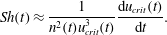 $$\begin{eqnarray}Sh(t)\approx \frac{1}{n^{2}(t)u_{crit}^{3}(t)}\frac{\text{d}u_{crit}(t)}{\text{d}t}.\end{eqnarray}$$
As nucleation events occur, we know that the Sherwood number is well approximated by the equality in inequality (3.15). Using this, we define $n^{\ast }(\cdot )$
as the continuous function obtained from the upper bound on
$n^{\ast }(\cdot )$
as the continuous function obtained from the upper bound on $Sh$
in the critical case
$Sh$
in the critical case
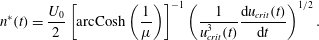 $$\begin{eqnarray}n^{\ast }(t)=\frac{U_{0}}{2}\left[\text{arcCosh}\left(\frac{1}{\unicode[STIX]{x1D707}}\right)\right]^{-1}\left(\frac{1}{u_{crit}^{3}(t)}\frac{\text{d}u_{crit}(t)}{\text{d}t}\right)^{1/2}.\end{eqnarray}$$
Clearly, $n^{\ast }(t)$
is in general not a natural number and may decrease. To obtain a discrete number of fluid domains, for any
$n^{\ast }(t)$
is in general not a natural number and may decrease. To obtain a discrete number of fluid domains, for any $t>0$
we take the maximum value (over time) of
$t>0$
we take the maximum value (over time) of $n^{\ast }$
rounded up to obtain
$n^{\ast }$
rounded up to obtain
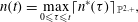 $$\begin{eqnarray}n(t)=\max _{0\leqslant \unicode[STIX]{x1D70F}\leqslant t}\lceil n^{\ast }(\unicode[STIX]{x1D70F})\rceil _{\mathbb{ P}^{2,+}},\end{eqnarray}$$
where $\lceil y\rceil _{\mathbb{P}^{2,+}}$
is the smallest integer power of
$\lceil y\rceil _{\mathbb{P}^{2,+}}$
is the smallest integer power of $2$
that is larger than
$2$
that is larger than $y$
. By definition,
$y$
. By definition, $n(\cdot )$
is a function from
$n(\cdot )$
is a function from $\mathbb{P}^{2,+}$
. Moreover, for any
$\mathbb{P}^{2,+}$
. Moreover, for any $t$
one has
$t$
one has $n(t)\geqslant n^{\ast }(t)$
, thus it is implied that melting processes are excluded. From equations (4.4) and (3.22) we can also recover the characteristic length
$n(t)\geqslant n^{\ast }(t)$
, thus it is implied that melting processes are excluded. From equations (4.4) and (3.22) we can also recover the characteristic length $\bar{\ell }$
.
$\bar{\ell }$
.
We emphasize the fact that due to the approximation in equation (3.22) this derivation is not exact. Its accuracy depends on whether and how fast the solution approaches the self-similar structure assumed up to now. This aspect is investigated numerically in § 5.3.
5 Numerical examples
In this section we present numerical solutions to the system of equations (2.10), derived in § 2.4. These solutions are computed by employing a cell-centred finite-volume method, which is presented in detail in appendix A.
We start with numerical experiments that investigate the regimes identified in § 3. First, in § 5.1 we verify that the system converges to the self-similar solution identified in equation (3.13) for the critical case. Second, we consider the super-critical regime using the external control proposed in equation (3.27). Finally, we verify the applicability of the discussed in § 4, both for an idealized case of external control provided by equation (3.27), as well as for a more challenging case with a logistic function controlling the freezing process.
5.1 Convergent solutions in the critical case
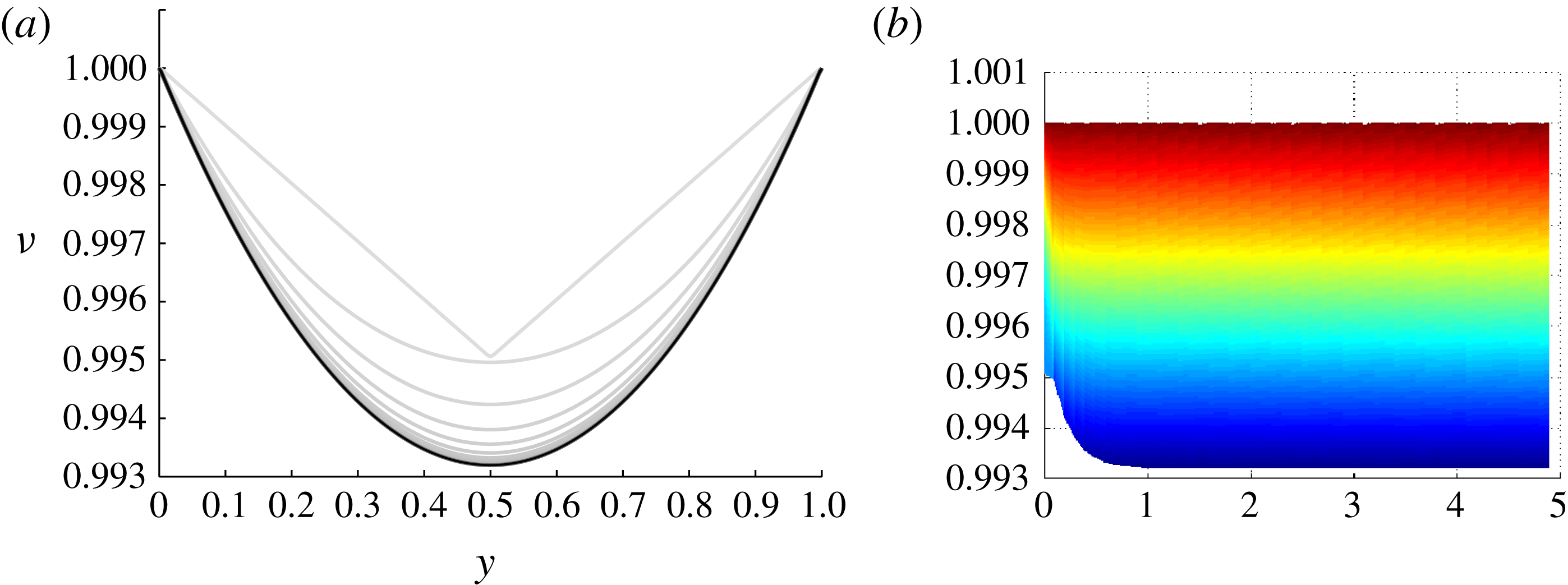
Figure 5. (a) The function $\unicode[STIX]{x1D708}$
at various times (darker colour corresponding to later time); (b) the solution surface plotted against dimensionless time.
$\unicode[STIX]{x1D708}$
at various times (darker colour corresponding to later time); (b) the solution surface plotted against dimensionless time.
We start by considering the self-similar salinity profile for the critical case derived in (3.10). Figure 5 presents the numerical results for the critical case. More precisely, it displays the scaled, dimensionless salinity $\unicode[STIX]{x1D708}$
introduced in (2.18). The initial condition in the numerical simulation is
$\unicode[STIX]{x1D708}$
introduced in (2.18). The initial condition in the numerical simulation is
 $$\begin{eqnarray}\unicode[STIX]{x1D708}(x,0)=0.01\cdot |x-.5|+.995,\quad \text{for }x\in [0,1],\end{eqnarray}$$
and the computation is for $Sh=0.5$
. As seen in figure 5(a), the numerical approximation eventually converges to the analytical solution (3.13).
$Sh=0.5$
. As seen in figure 5(a), the numerical approximation eventually converges to the analytical solution (3.13).
Figure 5(b) presents the solution in $\unicode[STIX]{x1D702}\times \unicode[STIX]{x1D708}$
axes. The lowest surface line in this projection illustrates the time evolution of
$\unicode[STIX]{x1D702}\times \unicode[STIX]{x1D708}$
axes. The lowest surface line in this projection illustrates the time evolution of $\min (u)/\max (u)=\min (\unicode[STIX]{x1D708})$
, that is, the quantity which will trigger secondary nucleation if it drops below the nucleation multiplier
$\min (u)/\max (u)=\min (\unicode[STIX]{x1D708})$
, that is, the quantity which will trigger secondary nucleation if it drops below the nucleation multiplier $\unicode[STIX]{x1D707}$
defined in (2.9). Thus the simulations reported here are valid for any
$\unicode[STIX]{x1D707}$
defined in (2.9). Thus the simulations reported here are valid for any $\unicode[STIX]{x1D707}\leqslant 0.993$
.
$\unicode[STIX]{x1D707}\leqslant 0.993$
.
The convergence of the solution to the self-similar profile predicted by theory indicates that the self-similar solution $\unicode[STIX]{x1D708}$
is robust with respect to perturbations, an observation which is supported by other calculations not shown herein.
$\unicode[STIX]{x1D708}$
is robust with respect to perturbations, an observation which is supported by other calculations not shown herein.
5.2 The numerical validation of the fractal-forming behaviour
The numerical experiments in this subsection verify that the condition for the external control on the critical salinity given in equation (3.27) indeed leads to binary, Cantor-set-type, fractals. This numerical approach is particularly important since in the super-critical fractal case it is not feasible to obtain an explicit self-similar solution as for the critical case. For this example we use $Sh(0+)=0.02$
, which is consistent with a nucleation threshold of
$Sh(0+)=0.02$
, which is consistent with a nucleation threshold of $0.9925$
according to inequality (3.15). The fractal formation is then characterized by the balance between freezing and nucleation, which we set to
$0.9925$
according to inequality (3.15). The fractal formation is then characterized by the balance between freezing and nucleation, which we set to $\unicode[STIX]{x1D706}=1.03$
for the sake of illustration.
$\unicode[STIX]{x1D706}=1.03$
for the sake of illustration.
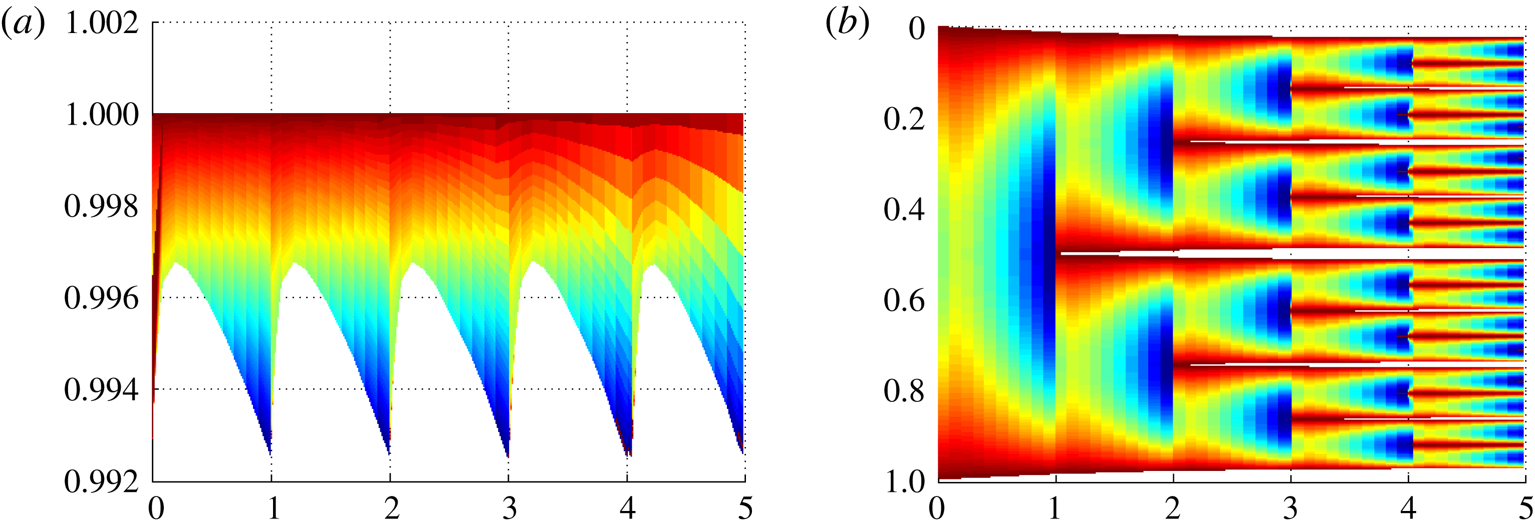
Figure 6. Demonstration of the fractal-forming behaviour for the super-critical conditions given in equation (3.27). Panel (a) shows minimum concentration (lower bound) and concentration profiles (colours), while (b) shows the concentration (colours) plotted on the domains as they split, thus white represents ice. For both panels, time is given with respect to the transformed time $\unicode[STIX]{x1D702}$
.
$\unicode[STIX]{x1D702}$
.
The salinity profile immediately after nucleation events converges towards an asymmetric self-similar solution after a few nucleation events and thus the initial condition is immaterial for the asymptotic behaviour of the system. To reflect this, we only show the solution after it has converged to the self-similar profile, typically within two to three splitting steps. The self-similar profile obtained in this example is also used as the initial condition of salinity when we return to exploring the non-asymptotic regimes in § 5.3.
The solution is shown in figure 6 for a time span covering several nucleation events. As the numerical simulation evidences, each sub-domain splits into two equal sub-domains with a period 1 in the nonlinear time $\unicode[STIX]{x1D702}$
. This provides a post hoc justification of the assumptions stated in § 3.2.
$\unicode[STIX]{x1D702}$
. This provides a post hoc justification of the assumptions stated in § 3.2.
The self similarity of the solution implies that the process will continue as $\unicode[STIX]{x1D702}\rightarrow \infty$
, leading to a countable infinity of splittings within a finite time (recall that
$\unicode[STIX]{x1D702}\rightarrow \infty$
, leading to a countable infinity of splittings within a finite time (recall that $t_{\infty }$
is finite). This results in a bipartite tree of sub-domains that, at each time, is an approximation of a Cantor-like set. We have verified this behaviour for freezing rates of
$t_{\infty }$
is finite). This results in a bipartite tree of sub-domains that, at each time, is an approximation of a Cantor-like set. We have verified this behaviour for freezing rates of $\unicode[STIX]{x1D706}=1.01$
to
$\unicode[STIX]{x1D706}=1.01$
to $\unicode[STIX]{x1D706}=1.50$
, the results of which are summarized in figure 7.
$\unicode[STIX]{x1D706}=1.50$
, the results of which are summarized in figure 7.

Figure 7. This log–log plot summarizes the relationship between remaining fluid fraction and characteristic fluid domain size. The linear trends (in log–log space) confirm the fractal structure of the solution over the full range of freezing rates.
5.3 Applying the approximate method to determine the properties of sea ice
In this subsection we validate the heuristically derived Sherwood number $Sh$
and mean brine-sub-domain length scale
$Sh$
and mean brine-sub-domain length scale $\ell$
derived in § 4. We use this opportunity to consider the pre-asymptotic regime alluded to in the previous section.
$\ell$
derived in § 4. We use this opportunity to consider the pre-asymptotic regime alluded to in the previous section.
5.3.1 Fractal solutions including the pre-asymptotic regime

Figure 8. Comparison of simulated and estimated Sherwood number and average sub-domain size for a solution including the pre-asymptotic regime.
We consider the asymmetric initial condition (from § 5.2) leading to initial asymmetrical splitting and thus the different brine sub-domains have different widths. In this case, the fractal does not have a pure binary structure anymore. This can be seen in figure 8, where each individual branch of the solution approaches an asymptotic regime after about four splittings. Note that for these figures we choose to use dimensionless time $t$
rather than
$t$
rather than $\unicode[STIX]{x1D702}$
and, to better visualize the results, we use
$\unicode[STIX]{x1D702}$
and, to better visualize the results, we use $t-t_{\infty }$
as the
$t-t_{\infty }$
as the $x$
-axis with logarithmic scale.
$x$
-axis with logarithmic scale.
As the numerical solution is driven by a prescribed $u_{crit}(t)$
, as detailed in § 5.2, we can apply the estimates for the mean length scale as well as the Sherwood numbers, as given by equations (3.22), (4.2) and (4.4). The estimates are compared against the true values obtained from the simulation in the lower part of figure 8. Since the estimate from § 4 does not know the initial salinity distribution, it cannot capture the details at the earliest stage of the simulation. However, for later times we find a reasonable agreement between the estimated and simulated values.
$u_{crit}(t)$
, as detailed in § 5.2, we can apply the estimates for the mean length scale as well as the Sherwood numbers, as given by equations (3.22), (4.2) and (4.4). The estimates are compared against the true values obtained from the simulation in the lower part of figure 8. Since the estimate from § 4 does not know the initial salinity distribution, it cannot capture the details at the earliest stage of the simulation. However, for later times we find a reasonable agreement between the estimated and simulated values.
5.3.2 A generic rapid freezing scenario
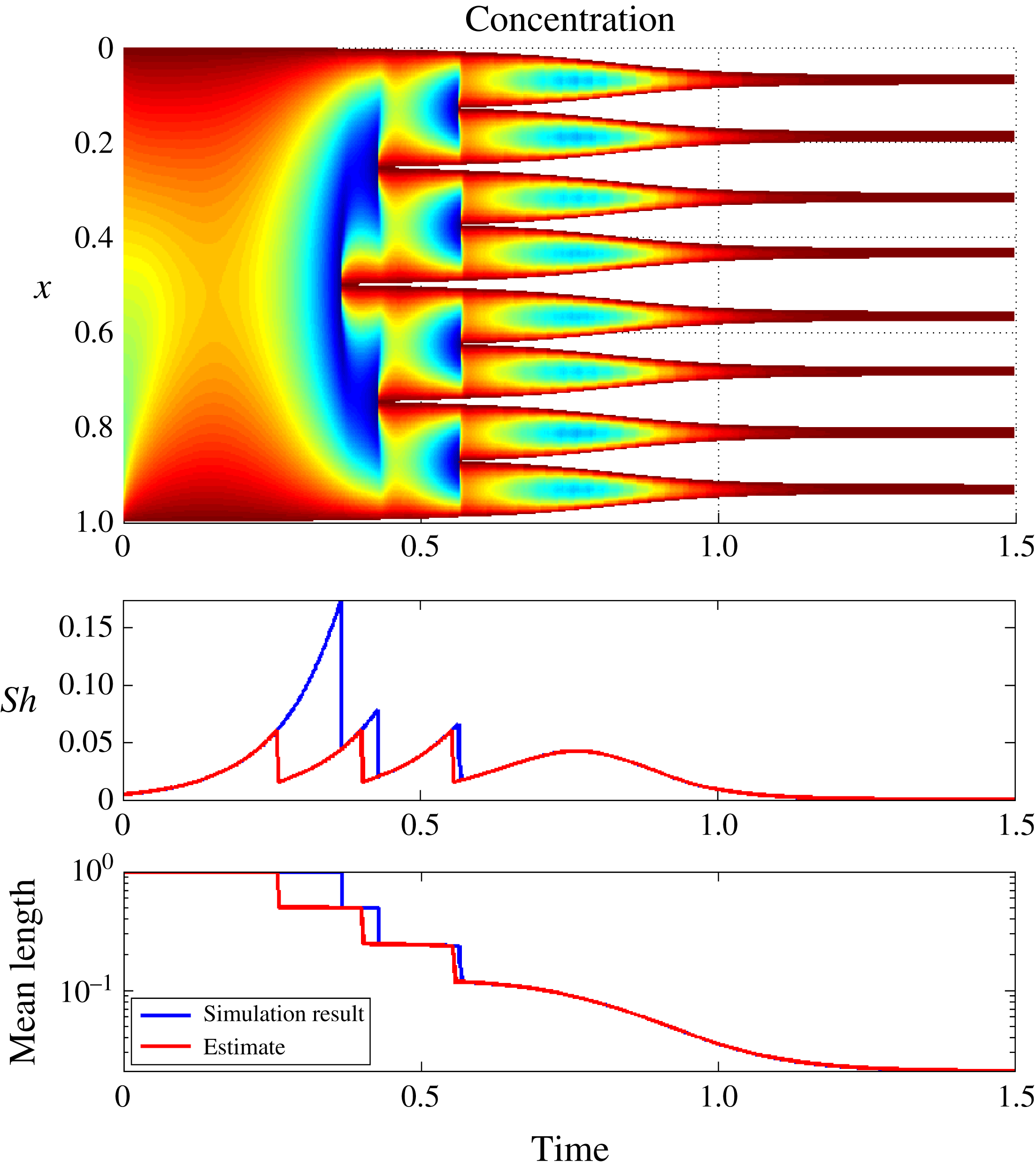
Figure 9. Comparison of simulated and estimated Sherwood number and average sub-domain size for logistic function boundary conditions.
As a final comparison, we consider a case of rapid freezing where the boundary salinity controlling the freezing process does not follow the monomial scaling given in equation (3.27). In particular, we consider the logistic function
 $$\begin{eqnarray}u_{crit}(t)=1+\frac{5}{(1+\exp (10(-t+1)))},\quad \text{for }t\in [0,1.5].\end{eqnarray}$$
This choice is motivated by the transition from a slow, diffusion-dominated regime via a nucleation-dominated regime and finally a diffusion-dominated regime. Paired with the non-symmetric initial conditions from § 5.2, we consider this a challenging test for the heuristic estimates derived in § 4.
The numerical solution and the comparison of the characteristic parameters are depicted on figure 9. We first note the rapid establishment of an asymptotic-like fractal structure, in the sense of the division of the original brine domain into eight nearly equal-sized partitions. This provides additional support to the applicability of the analysis of § 3 for general freezing regimes.
Second, we note from the lower figures that the estimates for characteristic brine-domain length and Sherwood number are in general very close to the computed values. Again the discrepancy is related to the salinity distribution at the onset of the freezing process, which is not captured, leading to a prediction of premature nucleation. As the nucleation process is established, the estimates approach the calculated values both of Sherwood number and of domain-size, with the correct prediction of eight fluid domains. As expected, the heuristic algorithm gives a very close match for the final smooth regime (starting from $t\approx 0.7$
) where the solution is close to the steady state.
$t\approx 0.7$
) where the solution is close to the steady state.
6 Conclusions
In this paper we have presented a mathematical model for ice-formation in brine. We avoid mushy-layer approximations and formulate the model explicitly in terms of the phase change (ice–brine) encountered at the lowest continuum scale.
In the 1D setting, we identify three freezing regimes: a sub-critical (slow) freezing regime where a continuous ice domain is formed; a critical regime when self-similar profiles are determined explicitly; and a super-critical (fast) freezing regime leading to fractal-like structures. The main contribution of the work is the explicit characterization of the critical regime, which represents the transition between continuous and fractal freezing.
Based on the characterization of the critical regime, we give a structural understanding of supercritical (nucleation-dominated) freezing, and derive closed-form estimates of characteristic ice-domain length scales for the whole time-dependent freezing process. These latter estimates form the initial steps towards a more rigorous understanding of the link between freezing conditions and physical parameters for the resulting porous structure.
A finite volume method is proposed for solving the moving-boundary models posed at the smallest scale. This numerical approach is used to verify the exact solution obtained in the critical regime. Under the fractal-behaviour conditions obtained in the super-critical regime, the numerical solution shows the expected nucleation process approaching a Cantor-set-like fractal structure.
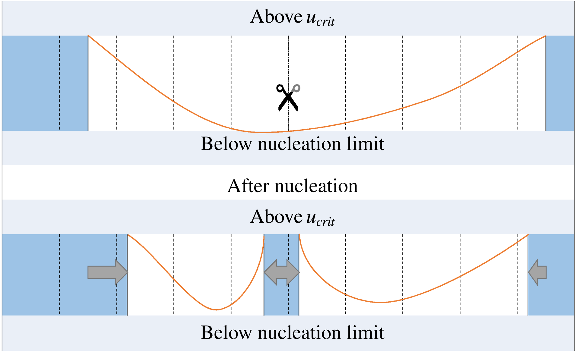
Figure 10. Scheme illustrating the finite difference method, including the occurrence of spontaneous nucleation. Dashed lines represent the boundaries of the grid cells. The sub-domains occupied by the solid are filled, the scissors indicate the place where splitting occurs due to nucleation, the arrows show how the ice domain has expanded.
Acknowledgements
S.A. thanks A. Kvashchuk for useful discussions during preparation of the manuscript and B. Balakin for helpful references. J.M.N. visited the Isaac Newton programme ‘Melt in the Mantle’ at Cambridge University while working on this manuscript. I.S.P. acknowledges support from the Akademia grant of Statoil and from the Research Foundation – Flanders FWO through the the Odysseus programme grant G0G1316N. The authors also acknowledge the feedback from the editor and reviewers that helped to improve the presentation of the paper.
Appendix A
This appendix presents the numerical method used to solve the model equations on the scale of a single brine domain. Also the method is verified against the self-similar solution obtained in the critical case.
A.1 Finite difference method
To obtain a numerical solution for the 1D model in § 2 we have modified a standard finite volume method with an explicit Euler time stepping.
Due to the ice domains acting as barriers, the scheme only needs to account for a single brine domain – multiple domains are handled by recursively calling new instances of the scheme. It is therefore sufficient for the numerical method to handle (i) diffusion of salt in the brine phase, (ii) motion of ice interfaces and (iii) nucleation events. The diffusion of salt in the brine phase is standard and will not be discussed further.
The motion of ice interfaces is necessary to resolve on a sub-grid scale. Thus, as indicated in figure 10, the ice domain is permitted to partially enter cells and these cells thus have an internal variable indicating the ice content. It is important to note that the boundary cells have a prescribed salt concentration and it is imperative that the mass balance relations for diffusion out of the boundary cell is solved together with the propagation of the ice boundary. The scheme allows for the ice to completely fill a cell during a time step and continue into the neighbouring cell. In that case an additional cell is used for finite difference stencil computation.
Finally, nucleation events are explicitly resolved. Whenever the nucleation limit is reached in a cell, the domain is split at the cell interface. The scheme chooses the interface that is the closest to the minimum of interpolated concentration. Starting from the next step the regions are treated independently.


 Open access