


1. Introduction
Odd viscous liquids are dissipationless in the sense that they do not give rise to viscous heating (Landau & Lifshitz Reference Landau and Lifshitz1987). They were systematically studied by Avron (Reference Avron1998), following previous work on the quantum Hall effect (Avron, Seiler & Zograf Reference Avron, Seiler and Zograf1995). Their constitutive laws, however, were already known in the context of polyatomic gases where a detailed experimental and theoretical program was performed at Leiden with a terminus ante quem in the 1960s (Beenakker & McCourt Reference Beenakker and McCourt1970; Hulsman et al. Reference Hulsman, van Waasdijk, Burgmans, Knaap and Beenakker1970). Recent experiments established the existence of odd viscosity in active liquids, which acted to suppress surface undulations in a manner resembling surface tension (Soni et al. Reference Soni, Bililign, Magkiriadou, Sacanna, Bartolo, Shelley and Irvine2019). In addition to the odd viscosity coefficients cited in the above works, there are others that may appear in materials endowed with discrete symmetries cf. (Rao & Bradlyn Reference Rao and Bradlyn2020; Souslov, Gromov & Vitelli Reference Souslov, Gromov and Vitelli2020). The review article by Fruchart, Scheibner & Vitelli (Reference Fruchart, Scheibner and Vitelli2023) discusses the above experiments and various physical effects that arise in the presence of odd viscosity.
A previously observed odd viscosity-induced uncommon physical effect, related to the corpus of the present paper, is the propagation of inertial-like waves in a three-dimensional odd viscous liquid. This is the case because such a liquid is endowed with an intrinsic mechanism that tends to restore a fluid particle back to its equilibrium position. In addition, a body moving slowly in a quiescent three-dimensional odd viscous liquid will be accompanied by a liquid cylindrical column whose generators circumscribe the body (Kirkinis & Olvera de la Cruz Reference Kirkinis and Olvera de la Cruz2023a).
The main result of this paper is the determination of wall and body-like modes in a rigidly rotating odd viscous liquid with angular velocity  $\varOmega$ in a disk or a cylinder of radius $R$ with no-slip boundary conditions that resemble their non-odd counterparts in rotating Rayleigh–Bénard convection (Goldstein et al. Reference Goldstein, Knobloch, Mercader and Net1993; Knobloch Reference Knobloch1994). We identify the wall modes with evanescent waves and the body modes with oscillatory inertial-like waves. Both types can be classified with respect to a single planar wavenumber $\kappa$, which is complex or real, respectively, cf. figure 1. These waves precess in a prograde or retrograde manner with respect to the rotating frame. Wall modes are prominent close to a solid boundary and body modes in the interior of the cylinder (or disk). An odd viscous liquid provides a third case where admissible wavenumbers $\kappa$ are concurrently real and imaginary, which we call ‘mixed’ in this paper. The classification of the physical behaviours according to the character of $\kappa$ is displayed in table 1.

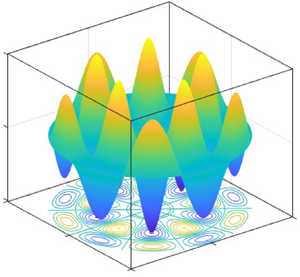
Figure 1. Wall and body modes (or evanescent and oscillatory inertial-like waves, respectively), and mixed mode of the fields (density or pressure  $\sim {\rm J}_m(\kappa r)$, where ${\rm J}_m$ is the Bessel function of the first kind and $m$ an integer determining periodicity in the azimuthal direction), for a rigidly rotating odd viscous liquid with angular velocity $\varOmega$, in two and three dimensions, satisfying no-slip boundary conditions. Each mode can be classified according to the character of the planar wavenumber $\kappa$, cf. table 1. Body modes: prominent in the interior of the cylinder. Wall modes: prominent near the side wall. Mixed modes: a combination of the previous two behaviours.
Table 1. Types of roots  $\kappa$ displayed in figure 3, from (2.12) $\nu _o\kappa ^2 = \alpha \pm \sqrt {\alpha ^2 + \beta }$ according to the sign of the parameters $\alpha = {\omega ^2}/{2\varOmega _o} - 2\varOmega$ and $\beta = \omega ^2 - (2\varOmega )^2$ defined in (2.13a,b). The last column defines the terminology employed in this paper to describe the physical effect.

Following the theory developed by Goldstein et al. (Reference Goldstein, Knobloch, Mercader and Net1993) and Knobloch (Reference Knobloch1994), we obtain the (exact) fields by satisfying the (no-slip in this paper) boundary conditions. This method provides the admissible curves in the parameter space spanned by the precession frequency  $\omega$ and odd viscosity coefficient $\nu _o$, giving rise to the aforementioned behaviour. Thus, it is possible to theoretically determine the largely unknown values of the odd viscosity coefficients by experimentally observing the frequency $\omega$ of the precessing patterns.
Recent studies on equatorial (Tauber, Delplace & Venaille Reference Tauber, Delplace and Venaille2019) and topological waves (Souslov et al. Reference Souslov, Dasbiswas, Fruchart, Vaikuntanathan and Vitelli2019) in two-dimensional odd viscous liquids provided examples of the bulk–interface correspondence by establishing the presence of topological waves at frequencies  $\omega <2\varOmega$. Our formulation recovers these effects as special cases.
This paper is thus organized as follows. In § 2.1, we formulate the non-axisymmetric motion of a two-dimensional compressible rigidly rotating odd viscous liquid in a disk geometry of radius  $R$ following the arguments developed earlier for (non-odd) rotating Rayleigh–Bénard convection (Goldstein et al. Reference Goldstein, Knobloch, Mercader and Net1993; Knobloch Reference Knobloch1994) and by Chandrasekhar (Reference Chandrasekhar1961). The variable part of the density $\rho '$ satisfies a scalar Poincaré–Cartan equation which leads to a relation between the planar wavenumber $\kappa$, material parameters and precession frequency $\omega$ in parameter space. Only one of these wavenumbers $\kappa$ is however admissible; it can be determined by solving a secular equation obtained by satisfying the (no-slip here) boundary conditions on the sidewall. Thus, the density profiles so obtained are precessing with frequency $\omega$ in the rotating frame of the disk and can be exponential or oscillatory in the radial direction. The radially exponential profiles are evanescent waves and resemble the wall modes obtained in (non-odd) rotating Rayleigh–Bénard convection (Goldstein et al. Reference Goldstein, Knobloch, Mercader and Net1993; Knobloch Reference Knobloch1994), although the wall modes of the latter system are a consequence of thermal forcing and supercritical behaviour of a non-odd system endowed with shear viscosity. The radially exponential profiles can also be understood as equatorial (Tauber et al. Reference Tauber, Delplace and Venaille2019) and topological waves (Souslov et al. Reference Souslov, Dasbiswas, Fruchart, Vaikuntanathan and Vitelli2019) (that is, waves that propagate parallel to a boundary and decay away from it exponentially). Solution of the real and imaginary parts of the secular equation gives parametric curves of admissible $(\omega, \nu _o)$ values (where $\nu _o$ is the coefficient of kinematic odd viscosity) leading to the aforementioned exponential/wall mode/evanescent behaviour. Therefore, this formulation can provide the means of determining the largely unknown odd viscosity coefficient by observing the precessing rate of patterns in an experiment. The special case of the axisymmetric $m=0$ mode is relegated to the supplementary materials available at https://doi.org/10.1017/jfm.2024.791. that includes a number of illustrative examples associated with this mode.
In § 3, we formulate the non-axisymmetric motion of a three-dimensional incompressible rigidly rotating odd viscous liquid in a cylinder of radius  $R$. The formulation is nearly identical to the two-dimensional case of § 2.1 with the exception of the presence of an axial velocity component $v_z(r,\phi,z,t)$, whose arguments are expressed with respect to cylindrical coordinates, and two (rather than one) odd viscosity coefficients $\nu _o$ and $\nu _4$. A Poincaré–Cartan and a secular equation give rise to the admissible planar real or complex wavenumbers $\kappa$ leading to precessing body and wall modes, respectively. Since the patterns precess in the rotating frame, again, one could determine the unknown odd viscosity coefficients by experimentally observing their rotation rate. The observation of evanescent waves in rigidly rotating (non-odd) inviscid or viscous liquids is rather rare with the exception of a recent experimental study (Nosan et al. Reference Nosan, Burmann, Davidson and Noir2021) and references therein. We thus adapt the experimental conditions of Nosan et al. (Reference Nosan, Burmann, Davidson and Noir2021) to the case of a three-dimensional odd viscous liquid rotating rigidly with angular velocity $\varOmega$. We show that fluid particle paths are ellipses lying on $r\unicode{x2013}z$ planes and can possibly be employed to determine the unknown values of the odd viscosity coefficients.
The two- and three-dimensional problems are formally equivalent and the density  $\rho '$ of the former plays the same role as the axial velocity component $v_z$ in the latter, as discussed in § 3.2. This behaviour is related to the conservation of helicity which is a consequence of the alignment of velocity with vorticity. This tendency of the two fields to alignment, even when nonlinear terms of the Navier–Stokes equations are included, is expected from general grounds (Pelz et al. Reference Pelz, Yakhot, Orszag, Shtilman and Levich1985). We relegate this discussion to the supplementary materials.
The effects described in the main body of this paper are affected by the lower order terms of the governing partial differential equations (the dispersion relation). We show in Appendix B how higher order terms are responsible for the propagation of data in directions explicitly determined by the values taken by the odd viscosity coefficients.
2. Evanescent and inertial-like oscillations in a rigidly rotating compressible two-dimensional odd viscous liquid
2.1. Non-axisymmetric waves
A two-dimensional odd viscous liquid obeys the constitutive law (Lapa & Hughes Reference Lapa and Hughes2014; Banerjee et al. Reference Banerjee, Souslov, Abanov and Vitelli2017; Ganeshan & Abanov Reference Ganeshan and Abanov2017)
 \begin{equation} \boldsymbol{\sigma}' = \eta_o \left(\begin{array}{@{}cc@{}} -\left(\partial_r v_\phi - \dfrac{1}{r}v_\phi + \dfrac{1}{r}\partial_\phi v_r \right) & \partial_r v_r - \dfrac{1}{r}v_r - \dfrac{1}{r}\partial_\phi v_\phi \\ \partial_r v_r - \dfrac{1}{r}v_r - \dfrac{1}{r}\partial_\phi v_\phi & \partial_r v_\phi - \dfrac{1}{r}v_\phi + \dfrac{1}{r}\partial_\phi v_r \end{array} \right), \end{equation}
where  $\eta _o$ is termed the odd viscosity coefficient. We here consider a two-dimensional compressible liquid rigidly rotating with angular velocity $\varOmega$, endowed with the above constitutive relation and satisfying the continuity equation
 \begin{equation} \partial_t \rho' + \rho\,\textrm{div} \,\boldsymbol{v} =0 \quad \textrm{for} \ \rho'\ll\rho, \end{equation}
where  $\rho '$ is the variable part of the density and $\rho$ a constant background level. In plane polar coordinates $r, \phi$ (cf. figure 2), consider azimuthally dependent fields of the form
 \begin{equation} \left[v_r(r), v_\phi(r), \rho'(r)\right] \exp({{\rm i}(m\phi -\omega t)}), \end{equation}
where  $\omega$ is a real frequency and $m$ an integer. Employing the constitutive law (2.1), the linearized equations of motion and continuity, in the frame of reference rotating with the liquid (Lifshitz & Pitaevskii Reference Lifshitz and Pitaevskii1981, § 89), become
 $$\begin{gather} -{\rm i}\omega v_r ={-}\frac{c^2}{\rho}\frac{\partial \rho'}{\partial r} + 2\varOmega v_\phi - \nu_o\left[ \mathcal{L} v_\phi + \frac{2{\rm i}m}{r^2} v_r\right], \end{gather}$$
 $$\begin{gather}-{\rm i}\omega v_\phi ={-}\frac{{\rm i}m c^2}{r}\frac{\rho'}{\rho}-2\varOmega v_r + \nu_o\left[ \mathcal{L} v_r - \frac{2{\rm i}m}{r^2} v_\phi \right], \end{gather}$$
 $$\begin{gather}-{\rm i}\omega \rho' ={-}\rho \left[ \frac{1}{r} \frac{\partial}{\partial r} \left( r v_r\right) + \frac{{\rm i}m}{r} v_\phi \right], \end{gather}$$
where  $c$ is the speed of sound, $\nu _o=\eta _o/\rho$ and $\mathcal {L}$ is the linear operator
 \begin{equation} \mathcal{L} = \nabla_2^2 -\frac{1}{r^2}, \end{equation}
where  $\nabla ^2_2$ is the two-dimensional Laplacian $({1}/{r})({\partial }/{\partial r}) ( r( {\partial }/{\partial r})) - {m^2}/{r^2}$ and we neglected the nonlinear terms assuming small-amplitude motions.

Figure 2. Two-dimensional odd viscous compressible liquid rotating with angular velocity  $\varOmega$. In plane polar coordinates, the velocity field is ${\boldsymbol {v}} = v_r \hat {{\boldsymbol {r}}} + v_\phi \hat {\boldsymbol {\phi }}$ in the frame rotating with the liquid at constant angular velocity $\varOmega$.
We impose no-slip boundary conditions at  $r=R$ as
 \begin{equation} v_r(r=R) = v_\phi(r=R) =0. \end{equation}
These can be relaxed and replaced by mixed no-slip and force-free boundary conditions as reported by Souslov et al. (Reference Souslov, Dasbiswas, Fruchart, Vaikuntanathan and Vitelli2019).
In Appendix C, we reduce the momentum and continuity equations into a single equation for the density  $\rho '$:
 \begin{equation} \partial_t\left[ \left(2\varOmega - \nu_o\nabla_2^2\right)^2 - c^2 \nabla_2^2 + \partial_t^2 \right] \rho' =0. \end{equation}
Substituting
 \begin{equation} \rho'(r,\phi) = {\rm J}_m(\kappa r) \exp({{\rm i}(m\phi -\omega t)}) \end{equation}
into (2.9), where  ${\rm J}_m$ is the Bessel function of first kind, we obtain the relation
 \begin{equation} {-}\kappa^{4} \nu_o^{2}-4 \varOmega \kappa^{2} \nu_o -c^{2} \kappa^{2}-4 \varOmega^{2}+\omega^{2} =0, \end{equation}
satisfied by the (possibly complex) wavenumber  $\kappa =\kappa (c, \varOmega,\omega, \nu _o)$, where all parameters in the round brackets are real. Solving (2.11) for $\kappa ^2$ leads to
 \begin{equation} \nu_o\kappa^2 = \alpha \pm \sqrt{\alpha^2 + \beta}, \end{equation}
where
 \begin{equation} \alpha ={-}\frac{c^2}{2\nu_o} - 2\varOmega, \quad \beta = \omega^2 - (2\varOmega)^2. \end{equation}
Therefore,  $\kappa$ in (2.12) can be real, imaginary or complex as displayed in figure 3 and table 1. Each one of these three root types thus corresponds to the three density or pressure behaviours depicted in figure 1.


From this point onwards, we follow the solution method employed by Goldstein et al. (Reference Goldstein, Knobloch, Mercader and Net1993) in determining the fields arising in non-odd rapidly rotating Rayleigh–Bénard convection. From the four values of  $\kappa$ obtained in (2.12), only two give rise to linearly independent solutions. Let $\kappa _1$ and $\kappa _2$ denote these $\kappa$ values. The fields can then be stated as
 \begin{equation} \left(\begin{array}{@{}c@{}} v_r \\ v_\phi \end{array} \right) = \sum_{j=1}^2 A_j\gamma_j \left( \begin{array}{@{}cc@{}} \delta_j & 2\varOmega \\ -2\varOmega & \delta_j \end{array} \right) \left( \begin{array}{@{}c@{}} \partial_r \\ \dfrac{{\rm i}m}{r} \end{array} \right){\rm J}_m(\kappa_j r), \quad \rho' = \sum_{j=1}^2A_j{\rm J}_m(\kappa_j r), \end{equation}
where the coefficients  $\gamma _j$ and $\delta _j$ are
 \begin{equation} \gamma_j = \frac{\kappa_j^{2} \nu_o +2 \varOmega}{2 \varOmega \kappa_j^{2} \rho}, \quad \delta_j = \frac{-2 {\rm i} \omega \varOmega}{\nu_o \kappa_j^{2}+2 \varOmega}, \quad j=1,2, \end{equation}
determined by substituting the solution (2.14a,b) into the continuity equation (2.6) and into the  $z$ component of the vorticity equation, and $A_j$ are complex constants determined by the boundary conditions. Substituting (2.14a,b) into the boundary conditions (2.8) leads to a homogeneous system for two (complex) equations for the $A_i$,
 \begin{equation} \boldsymbol{M}(\nu_o, \omega, \varOmega, c, \rho, m, R) \left( \begin{array}{@{}c@{}} A_1\\ A_2 \end{array} \right) =0. \end{equation}
The complex matrix  $\boldsymbol {M}$ also depends on $\kappa _j$ through the dispersion relation. System (2.16) has a solution only when its determinant vanishes, explicitly when
 \begin{equation} \textrm{det} \,\boldsymbol{M} \equiv v_r(\kappa_1R) v_\phi(\kappa_2 R) - v_r(\kappa_2R) v_\phi (\kappa_1R) =0. \end{equation}
We thus parametrize  $\kappa _1(\omega, \nu _o)$ and $\kappa _2(\omega, \nu _o)$, fix values for $\varOmega, c, \rho, m$ and $R$, substitute into the real and imaginary parts of the secular equation (2.17), and solve for $\omega$ and $\nu _o$.
2.2. Character of the eigenvalue  $\kappa$

Recent literature on two-dimensional compressible odd viscous liquids (Souslov et al. Reference Souslov, Dasbiswas, Fruchart, Vaikuntanathan and Vitelli2019; Tauber et al. Reference Tauber, Delplace and Venaille2019) has brought forward examples supporting the bulk–interface correspondence by establishing the presence of waves propagating parallel to a boundary and increasing/decreasing exponentially with distance from it. The starting point for these studies is the dispersion relation  $\omega = \omega ({\boldsymbol {k}})$ obtained from (2.11), where ${\boldsymbol {k}}$ is a real wavevector. In this case, dispersion curves exist only for $\omega >2\varOmega$. To obtain the exponential behaviour, the wavenumber then is set to be complex and the frequencies studied are those in the ‘gap’, that is, with $\omega <2\varOmega$.
We here adopt an opposite outlook, similar to the one followed in the literature of rigidly rotating liquids. This method emphasizes the derivation of a wavenumber  $\kappa$, as in (2.12), that can be complex and is a function of an always real frequency $\omega$.
We display in figure 4 the frequency  $\omega$ versus the real and imaginary parts of $\kappa$, drawn from (2.12) which is to be compared with figure 3 and table 1. In figure 4(a), when $\omega <2|\varOmega | = 40$ ( $\beta <0$), the four imaginary roots are clearly visible. When $\omega > 40 = 2|\varOmega |$ ( $\beta >0$), (2.12) acquires two real and two imaginary $\kappa$ roots. In figure 4(b), when $\omega <2|\varOmega | = 1000$ ( $\beta <0$), two distinct behaviours are visible. Those that make $\alpha ^2+\beta$ in (2.12) negative give rise to the aforementioned complex roots (located below the parabola of figure 3), while those that make $\alpha ^2+\beta$ positive give rise to four real roots (located outside the parabola of figure 3). When $\beta$ becomes positive ( $\omega >2|\varOmega | = 1000$), we obtain two imaginary and two real roots for $\kappa$.

Figure 4. Real frequency  $\omega$ versus the real and imaginary parts of the eigenvalue $\kappa$ derived as a solution of (2.12). Both panels emphasize the presence of imaginary or complex values of $\kappa$ that cannot be captured by a plane-wave analysis of the momentum equations. In particular, the domain $\omega <2\varOmega$ is populated by imaginary or complex $\kappa$ that may give rise to wall (evanescent wave) modes (the character of $\kappa$ is displayed in figure 3). Note that the indicated curves are symmetric with respect to the $\omega =0$ plane and continuously extend towards negative $\omega$ values. The parameters are given in arbitrary units. (a) $(c, \varOmega, \nu _o, \rho ) = (8, -20, 0.1, 1)$. (b) $(c, \varOmega, \nu _o, \rho ) = (15, -500, 2, 1)$.
The conclusion of this discussion is that values of the frequency  $\omega <2\varOmega$ exist when the wavenumber $\kappa$ is imaginary or complex, and this is a natural outcome of the present formulation. Note that both panels in figure 4 symmetrically extend for negative values of the frequency.
2.3. Basic observations
From (2.4)–(2.6), we can calculate the vorticity  $\textrm {curl}\,{\boldsymbol {v}} = ({1}/{r})[{\partial (r v_\phi )}/{\partial r} -{\partial v_r}/{\partial \phi }]\hat {{\boldsymbol {z}}}$ of the two-dimensional odd viscous liquid, which is found to be proportional to the density $\rho '$:
 \begin{equation} \textrm{curl}\,\boldsymbol{v} = (\kappa^2 \nu_o + 2\varOmega) \frac{\rho'}{\rho}\hat{\boldsymbol{z}}. \end{equation}
This proportionality was also pointed out in the numerical simulations of Souslov et al. (Reference Souslov, Dasbiswas, Fruchart, Vaikuntanathan and Vitelli2019, figure S2). On account of the equivalence of the two- and three-dimensional problem (to be discussed in § 3.2), this proportionality is justified based on the conservation of helicity. In addition, it is expected to persist, even when (the neglected here) nonlinear terms are incorporated into the Navier–Stokes equations (Pelz et al. Reference Pelz, Yakhot, Orszag, Shtilman and Levich1985). The conservation of helicity follows familiar lines and is thus relegated to the supplementary materials.
2.4. Wall and body modes in two-dimensional compressible odd viscous liquids
Goldstein et al. (Reference Goldstein, Knobloch, Mercader and Net1993) and Knobloch (Reference Knobloch1994), following the experiments of Ecke, Zhong & Knobloch (Reference Ecke, Zhong and Knobloch1992) in rapidly rotating Rayleigh–Bénard convection (of a non-odd liquid), showed theoretically the existence of two types of non-axisymmetric modes precessing in the rotating system: wall modes, which peak near the sidewall and decay in the interior of the cylinder, and body modes filling the whole cylinder and having their largest amplitudes close to the centre rather than the sidewall. Both types are classified in table 1. We proceed by showing that the two-dimensional compressible odd viscous liquid under consideration gives rise to similar wall and body modes which can be understood in the context of our formulation as evanescent and oscillatory inertial-like waves, respectively.
In figure 5(a,b), we display the density profiles for the wall modes  $m=2$ and $m=5$ arising by solving the system (2.17) in a disk of radius $R=10$ rotating with angular velocity $\varOmega = 20$ and $\omega >0$ in both cases (we employ arbitrary units). Thus, the profiles precess with frequency $\omega$ in a prograde manner in the frame rotating with the disk. Both profiles resemble those of the temperature distribution in (non-odd) rapidly rotating Rayleigh–Bénard convection as they are displayed in Goldstein et al. (Reference Goldstein, Knobloch, Mercader and Net1993, figure 6). Note also the resemblance of the contour plots in figure 5(c,d) to those of Souslov et al. (Reference Souslov, Dasbiswas, Fruchart, Vaikuntanathan and Vitelli2019, figure 3 and S3).

Figure 5. Density profiles and contours for the wall modes arising when the parameter  $\kappa$ lies in the lower left of the diagram in figure 3 (two imaginary pair $\kappa$ values) and thus the frequencies lie in the ‘gap’ $(-2\varOmega, 2\varOmega )$. (a,c) $m=2$ mode, with $(\omega, \nu _o) = (0.4, 6.4)$ as solution of system (2.17) leading to $(\kappa _1, \kappa _2) = (-1.95i, -3.2i)$. (b,d) $m=5$ mode, with $(\omega, \nu _o) = (1.5, 2.5)$ as a solution of system (2.17) leading to $(\kappa _1, \kappa _2) = (-2.7i, -5.9i)$. In both cases, $(c, \varOmega, \rho _0, R) = (8, 20, 1,10)$ and thus both profiles precess in a prograde manner in the frame rotating with the liquid. Note the resemblance of the density profiles with the temperature distribution of rapidly rotating (non-odd) Rayleigh–Bénard convection in Goldstein et al. (Reference Goldstein, Knobloch, Mercader and Net1993, figure 6) and of the contour plots with those of Souslov et al. (Reference Souslov, Dasbiswas, Fruchart, Vaikuntanathan and Vitelli2019, figures 3 and S3). Observing experimentally the precession rate of patterns could, in principle, lead to the determination of the odd viscosity coefficient. Parameter and observable units are arbitrary.
In figure 6, we display admissible  $(\nu _o, \omega )$ pairs, as a solution of system (2.17), giving rise to the wall modes displayed in figure 5. Thus, all the corresponding $\kappa$ values arising from the displayed parameter pairs are imaginary and will give rise to exponentially decaying velocity fields in the radial direction. Since the modes precess with frequency $\omega$ in the rotating frame, these modes will also propagate parallel to the circular boundary of the disk. It is thus clear that observing experimentally the precession rate of patterns could, in principle, lead to the determination of the odd viscosity coefficient $\nu _o$.

Figure 6. Admissible  $(\nu _o, \omega )$ pairs, as a solution of system (2.17), giving rise to the wall modes displayed in figure 5 employing the latter figure's parameter values. Thus, observing experimentally the precession rate of patterns $\omega$, it would be possible, in principle, to determine the largely unknown value of the odd viscosity coefficient $\nu _o$. Arbitrary units of the parameters were employed.
We note that Favier & Knobloch (Reference Favier and Knobloch2020) and Knobloch (Reference Knobloch2022) commented on the resemblance of wall modes in (non-odd) rapidly rotating Rayleigh–Bénard convection to odd viscosity-induced topological waves that appear near the boundary of a rotating two-dimensional odd viscous liquid (Souslov et al. Reference Souslov, Dasbiswas, Fruchart, Vaikuntanathan and Vitelli2019).
In figure 7, we display the density and contour profile of the body mode  $m=5$ arising by solving the system (2.17) in a disk of radius $R=10$ rotating with angular velocity $\varOmega = 20$. The profile precesses with frequency $\omega$ in a prograde manner in the frame rotating with the disk. The profile resembles somewhat the temperature distribution in the (non-odd) rapidly rotating Rayleigh–Bénard convection as they are displayed in Goldstein et al. (Reference Goldstein, Knobloch, Mercader and Net1993, figure 7).

Figure 7. A body mode for  $m=5$ with $(\omega, \nu _o) = (34.6,$ $-2.8)$ as a solution of system (2.17) leading to $(\kappa _1, \kappa _2) = ($ $-4.2, 1.7)$, and the same parameters as in figure 5. Thus, the admissible $\kappa$ values are located in the lower right of figure 3. The patterns precess in the rotating frame in a prograde manner. Note the resemblance of the density profiles with the temperature distribution of non-odd rapidly rotating Rayleigh–Bénard convection in Goldstein et al. (Reference Goldstein, Knobloch, Mercader and Net1993, figure 7). Observing experimentally the precession rate of patterns could, in principle, lead to the determination of the odd viscosity coefficient. Units employed above are arbitrary.
3. Inertial-like waves in a three-dimensional rigidly rotating incompressible odd viscous liquid
The constitutive law of an odd viscous liquid in three dimensions is of the form
 \begin{equation} \boldsymbol{\sigma}' = \boldsymbol{\sigma}_o' + \boldsymbol{\sigma}_4', \end{equation}
where, in cylindrical polar coordinates  $r, \phi, z$,
 \begin{equation} \boldsymbol{\sigma}_o' = \eta_o \left(\begin{array}{@{}ccc@{}} -\left(\partial_r v_\phi - \dfrac{1}{r}v_\phi + \dfrac{1}{r}\partial_\phi v_r \right) & \partial_r v_r - \dfrac{1}{r}v_r - \dfrac{1}{r}\partial_\phi v_\phi & 0\\ \partial_r v_r - \dfrac{1}{r}v_r - \dfrac{1}{r}\partial_\phi v_\phi & \partial_r v_\phi - \dfrac{1}{r}v_\phi + \dfrac{1}{r}\partial_\phi v_r & 0\\ 0 & 0 & 0 \end{array} \right) \end{equation}
and
 \begin{equation} \boldsymbol{\sigma}_4' = \eta_4 \left(\begin{array}{@{}ccc@{}} 0 & 0 & -\left(\dfrac{1}{r}\partial_\phi v_z + \partial_z v_\phi\right)\\ 0 & 0 & \partial_r v_z + \partial_z v_r\\ -\left(\dfrac{1}{r}\partial_\phi v_z + \partial_z v_\phi\right) & \partial_r v_z + \partial_z v_r & 0 \end{array} \right), \end{equation}
where  $\eta _o$ and $\eta _4$ are the odd viscosity coefficients. Notation employed in the literature to denote the odd viscosity coefficients appears in table 2.
Table 2. Conventions of odd viscosity coefficients that have appeared in the literature.

Consider a three-dimensional odd viscous liquid rotating rigidly about the  $\hat {{\boldsymbol {z}}}$ axis with angular velocity $\varOmega$ (cf. figure 8) and azimuthally dependent fields
 \begin{equation} \left[v_r(r), v_\phi(r),v_z(r) , p'(r)\right] \exp({{\rm i}(kz+m\phi -\omega t)}) \end{equation}
in the frame of reference rotating with the liquid, where the frequency  $\omega$ and wavenumber $k$ along the axis are both real and $m$ is an integer. We assume that $k$ has already been fixed by suitable boundary conditions on the lids of the cylinder. We neglect the nonlinear terms by assuming small-amplitude motions. The Navier–Stokes equations take the form
 $$\begin{gather} -{\rm i}\omega v_r -2\varOmega v_\phi ={-}\frac{1}{\rho}\frac{\partial p'}{\partial r} - \nu_o\left[ \mathcal{L} v_\phi + \frac{2{\rm i}m}{r^2} v_r\right] + \nu_4 \left[k^2 v_\phi + \frac{mk}{r} v_z\right] , \end{gather}$$
 $$\begin{gather}-{\rm i}\omega v_\phi + 2\varOmega v_r ={-}\frac{{\rm i}m}{r} \frac{p'}{\rho} + \nu_o\left[ \mathcal{L} v_r - \frac{2{\rm i}m}{r^2} v_\phi \right] + \nu_4 \left[{-}k^2 v_r + {\rm i}k \frac{\partial v_z}{\partial r} \right] , \end{gather}$$
 $$\begin{gather}-{\rm i}\omega v_z ={-}\frac{{\rm i}k}{\rho} \left[p' + \eta_4 \zeta \right], \end{gather}$$
where  $\mathcal {L}$ is the linear differential operator (2.7), $p'$ is the variable part of the pressure in the wave, $(\nu _o, \nu _4) \equiv ( \eta _o, \eta _4)/\rho$ are the coefficients of kinematic odd viscosity, $\zeta$ is the $z$ component of the vorticity, $\zeta = ({1}/{r})[{\partial }/{\partial r} ( r v_r) - {\rm i} m v_r ]$ and the centrifugal acceleration has been combined into the effective pressure $p'$ (Greenspan Reference Greenspan1968).

Figure 8. Three-dimensional odd viscous liquid rotating with angular velocity  $\varOmega$ about the $\hat {{\boldsymbol {z}}}$ axis. In cylindrical coordinates, the velocity field is ${\boldsymbol {v}} = v_r \hat {{\boldsymbol {r}}} + v_\phi \hat {\boldsymbol {\phi }} + v_z \hat {{\boldsymbol {z}}}$ in the frame of reference rotating with the liquid.
The incompressibility condition becomes
 \begin{equation} \frac{1}{r} \frac{\partial}{\partial r} \left( r v_r\right) +\frac{ {\rm i}m}{r} v_\phi+{\rm i}kv_z= 0. \end{equation}
 In Appendix B, we derive a single equation for the pressure  $\tilde {p} = p' + \eta _4 \zeta$,
 \begin{equation} \left[\nabla_2^2 + \left(1 - \frac{(2\varOmega - \mathcal{S})^2}{\omega^2}\right) \partial_z^2\right] \tilde{p} =0, \end{equation}
where  $\mathcal {S}$ is the linear operator
 \begin{equation} \mathcal{S} = (\nu_o-\nu_4)\nabla^2_2 + \nu_4\partial_z^2 , \end{equation} $\nabla ^2_2$ is the two-dimensional (horizontal) Laplacian and we considered perturbations of the pressure $\sim \exp (-{\rm i}\omega t)$ with real frequency $\omega$. Clearly, when $\nu _o = \nu _4 =0$, (3.9) reduces to the standard Poincaré–Cartan equation (A1) of non-odd rigidly rotating liquids.
Substituting
 \begin{equation} \tilde{p}(r,\phi) = {\rm J}_m(\kappa r) \exp({{\rm i}(kz+m\phi -\omega t)}) \end{equation}
into (3.9), where  ${\rm J}_m$ is the Bessel function of first kind, leads to a quartic equation for the determination of wavenumber $\kappa$:
 \begin{equation} {-}\kappa^{2}-k^{2} \left[1-\frac{\left(2 \varOmega +\nu_4 k^{2}+\left(\nu_o -\nu_4 \right) \kappa^{2}\right)^{2}}{\omega^{2}}\right] =0. \end{equation}
The  $\kappa$ solutions of (3.12) are given by the simple expression
 \begin{equation} \kappa^2 = \frac{\alpha \pm \sqrt{\alpha^2 + \beta}}{2(\nu_o - \nu_4)^2 k^2}, \end{equation}
with
 \begin{align} \alpha = \omega^{2}+2 k^{2} \left(\nu_4 -\nu_o \right) (2\varOmega + \nu_4 k^2), \quad \beta = 4k^4(\nu_o-\nu_4)^2\left[\omega^2 - (2\varOmega+\nu_4k^2)^2\right]. \end{align}
Thus, the character of  $\kappa$ values (real, imaginary or complex) is again described by figure 3 and table 1.
From the four values of  $\kappa$ obtained in (3.13), only two give rise to linearly independent solutions. Let $\kappa _1$ and $\kappa _2$ denote these $\kappa$ values. The fields can then be cast as
 \begin{equation} \left( \begin{array}{@{}c@{}} v_r \\ v_\phi \end{array} \right) = \sum_{j=1}^2 A_j\gamma_j \left( \begin{array}{@{}cc@{}} \delta_j & 2\varOmega \\ -2\varOmega & \delta_j \end{array} \right) \left( \begin{array}{@{}c@{}} \partial_r \\ \dfrac{{\rm i}m}{r} \end{array} \right){\rm J}_m(\kappa_j r), \quad v_z= \sum_{j=1}^2A_j{\rm J}_m(\kappa_j r), \end{equation}
the coefficients  $\gamma _j$ and $\delta _j$ are
 \begin{equation} \gamma_j = \frac{\kappa_j^{2} (\nu_o-\nu_4) +\nu_4k^2 + 2 \varOmega }{2 \varOmega \kappa_j^{2} \omega}, \quad \delta_j = \frac{-2 {\rm i} \omega \varOmega}{\kappa_j^{2} (\nu_o-\nu_4) +\nu_4k^2 + 2 \varOmega }, \quad j=1,2, \end{equation}
determined by substituting the solution (3.15a,b) into the isochoric constraint (3.8) and into the  $z$ component of the vorticity equation, and $A_j$ are complex constants to be determined by the boundary conditions.
We impose no-slip boundary conditions at the sidewall of the cylinder  $r=R$:
 \begin{equation} v_r(r=R) = v_\phi(r=R) =0, \end{equation}
leading to an homogeneous system for two (complex) equations for the  $A_i$,
 \begin{equation} \boldsymbol{M}(\nu_o, \nu_4,\omega, \varOmega, k, m, R) \left( \begin{array}{@{}c@{}} A_1\\ A_2 \end{array} \right) =0. \end{equation}
System (3.18) has a solution only when its determinant
 \begin{equation} \textrm{det} \,\boldsymbol{M} \equiv v_r(\kappa_1R) v_\phi(\kappa_2 R) - v_r(\kappa_2R) v_\phi (\kappa_1R) =0 \end{equation}
vanishes. We thus parametrize  $\kappa _1(\omega, \nu _o, \nu _4)$ and $\kappa _2(\omega, \nu _o,\nu _4)$, fix values for $\varOmega, k, R,m$, substitute into the real and imaginary parts of (3.19), and solve for $\omega$ and $\nu _o$ (see the discussion in § 3.3 on how $\nu _4$ is chosen).
3.1. Character of the $\kappa$ eigenvalues

A non-odd rotating liquid has  $\kappa$ solutions satisfying
 \begin{equation} \kappa = k\sqrt{\frac{4\varOmega^2}{\omega^2} -1} \quad \textrm{(non-odd rotating liquid)} \end{equation}
(obtained from the Poincaré–Cartan equation (A1)). Thus, when  $\omega <2\varOmega$, $\kappa$ is real and the solutions are oscillatory Bessel functions. When however $\omega >2\varOmega$, there are two imaginary $\kappa$ values and the fields are modified (exponentially increasing) Bessel functions.
We display in figure 9 the frequency  $\omega$ versus the real and imaginary parts of $\kappa$, drawn from (3.13) which is to be compared with figure 3 and table 1.

Figure 9. Real frequency  $\omega$ versus the real and imaginary parts of the eigenvalue $\kappa$ derived as a solution of (3.13). Both panels emphasize the presence of imaginary or complex values of $\kappa$ that cannot be captured by a plane-wave analysis of the momentum equations. In particular, the domain $\omega <2\varOmega$ is populated by imaginary or complex $\kappa$ values that exclusively give rise to wall (evanescent wave) modes. Note that the indicated curves are symmetric with respect to the $\omega =0$ plane. Units employed above are arbitrary. (a) $(\varOmega, \nu _o, k) = (5, 1, 1)$. (b) $(\varOmega, \nu _o, k) = (5, 10, 1)$.
In figure 9(a), we display the bifurcation diagram for the set of values  $(\varOmega, \nu _o, k) = (5, 1, 1)$ (arbitrary units). There are two complex conjugate roots up to $\omega = 6$, where the radical in (3.13) changes sign. For $6<\omega <10 = 2\varOmega$, there are four real roots and beyond this, two imaginary and two real roots. In figure 9(b), we employ the alternative set of values $(\varOmega, \nu _o, k) = (5, 10, 1)$ (arbitrary units). There are four imaginary $\kappa$ roots up to $\omega = 10 = 2\varOmega$. Beyond this, there are two imaginary and two real roots.
3.2. Formal equivalence of the two- and three-dimensional problems
Setting  $\nu _4=0$ in the equations of motion shows that they are equivalent to their two-dimensional counterparts by effecting the correspondence
 \begin{equation} p' = c^2 \rho' \textrm{ (2D)}, \quad p' = \frac{\rho \omega}{k} v_z \textrm{ (3D)}. \end{equation}
The pressure in the two- and three-dimensional cases satisfies  $p' = ({\rho c^2}/{{\rm i}\omega })\, \textrm {div}_2 {\boldsymbol {v}}$ and $p' =- ({\rho \omega }/{{\rm i}k^2})\, \textrm {div}_2 {\boldsymbol {v}}$, respectively, where $\textrm {div}_2 {\boldsymbol {v}} =({1}/{r}) [\partial _r (rv_r) + {\rm i}m v_\phi ]$. Thus, the two problems are identical inasmuch as the respective dispersion relations are taken into account.
Likewise, the three-dimensional problem with  $\nu _4 \neq 0$ can be recovered from the three-dimensional problem with $\nu _4 =0$ by performing the substitution
 \begin{equation} \nu_o \rightarrow \nu_o -\nu_4, \quad \textrm{and} \quad 2\varOmega \rightarrow 2\varOmega + \nu_4 k^2. \end{equation}
Thus, the role of  $\nu _4$ is to renormalize both the angular velocity $\varOmega$ and the odd viscosity coefficient $\nu _o$.
The question arises, if the two- and three-dimensional problems are mathematically equivalent, where do they differ? In the Appendix, we show that the role of  $\nu _4$ is to alter the direction of propagation of data along characteristics. For instance, when $\nu _4$ is zero, characteristics are parallel to the $z$ axis, giving rise to a Taylor column, while when $\nu _4$ is non-zero, they become oblique to the centre axis.
3.3. Mixed and body modes in a three-dimensional odd viscous liquid
In § 2.4, we illustrated the two-dimensional theory by deriving the density profiles when the wavenumbers  $\kappa$ were all imaginary or all real, thus respectively giving rise to wall and body modes defined in table 1, as these are displayed in figures 5 and 7, respectively. There is a third category however, as this is displayed by the character of wavenumbers $\kappa$ in the upper part of figure 3, where there are concurrent real and imaginary admissible $\kappa$ values as a solution of equation (2.12). Here we will provide one such example, which is displayed in figure 10(a,c).

Figure 10. Precessing axial velocity (or pressure) profiles and contours for the modes arising when the parameter  $\kappa$ lies in the upper part (two real two imaginary) and lower right section of the diagram in figure 3 (four real $\kappa$ values), respectively. (a,c) $m=2$ mixed mode, with $(\omega, \nu _o) = (-0.9, -3.3)$ as a solution of system (2.17) leading to $(\kappa _1, \kappa _2) = (-0.97, -0.5i)$. (b,d) $m=5$ body mode, with $(\omega, \nu _o) = (0.3,-3 )$ as a solution of system (2.17) leading to $(\kappa _1, \kappa _2) = (-0.75, 0.3)$. In both cases, $(k, \varOmega, R) = (1, 1, 10)$ in arbitrary units. The odd viscosity coefficients were chosen to satisfy $\nu _o=2\nu _4$, as explained in (3.23). Observing experimentally the precession rate of patterns could, in principle, lead to the determination of the odd viscosity coefficients $\nu _o$ and $\nu _4$. Units employed above are arbitrary.
In three dimensions, there are two odd viscosity coefficients and a choice has to be made regarding the solution of secular equation (3.19) (two equations for the determination of  $\omega, \nu _o$ and $\nu _4$). We thus follow (Markovich & Lubensky Reference Markovich and Lubensky2021; Khain et al. Reference Khain, Scheibner, Fruchart and Vitelli2022) who consider the combination
 \begin{equation} \eta_o = 2\eta_4 \end{equation}
as representing an experimentally verified case (for polyatomic gases, Hulsman et al. Reference Hulsman, van Waasdijk, Burgmans, Knaap and Beenakker1970). See the discussion of Kirkinis & Olvera de la Cruz (Reference Kirkinis and Olvera de la Cruz2023a, § 8.3) for some consequences of making this choice.
In figure 10(a,b), we display the axial velocity profiles for the mixed mode  $m=2$ and body mode $m=5$ arising by solving the system (3.19) in a cylinder of radius $R=10$ rotating with angular velocity $\varOmega = 1$, $k=1$, employing arbitrary units and enforcing the combination (3.23). Plotting the velocity component $v_z$ is equivalent to plotting the pressure $\tilde {p} = p' + \eta _4 \zeta$ on account of the connexion (3.7). Note that the non-vanishing $\nu _4$ has renormalized the cylinder angular velocity $\varOmega$ according to (3.21a,b), making $\beta = 8.3>0$ in (3.14a,b).
As in the two-dimensional case, the outcome of this formulation is to give some means of determining the odd viscosity coefficients by observing experimentally the precession rate of the patterns.
3.4. Evanescent waves in the experiments of Nosan et al. (Reference Nosan, Burmann, Davidson and Noir2021)
Consider an annular cylinder of inner and outer radii  $R_1$ and $R_2$, respectively, where the inner boundary is being radially displaced harmonically with frequency $\omega$. The liquid is rotating as a whole with angular velocity $\varOmega$ about the central axis. This then is a system with the geometry employed in the recent experiments of Nosan et al. (Reference Nosan, Burmann, Davidson and Noir2021) which showed that a (non-odd) rigidly rotating three-dimensional incompressible liquid gives rise to evanescent waves at the cross-over frequency $\omega \rightarrow 2\varOmega$. Setting $\omega = 2\varOmega$ ( $\beta =0$ in (3.13)), we obtain two imaginary roots $\kappa =\pm {\rm i}\tilde {\kappa }$ for real $\tilde {\kappa }$ from (3.13) if $0<\varOmega <\varOmega _o (\equiv \nu _ok^2)$ and the solution reads
 \begin{equation} v_r = A{\rm I}_1(\tilde{\kappa} r) + B{\rm K}_1(\tilde{\kappa} r), \end{equation}
where by  $\tilde {\kappa }$ in this section only, we denote the imaginary part of the roots of (3.13). Thus,
 \begin{equation} \tilde{\kappa} = 2\sqrt{\frac{\varOmega}{\nu_o} \left( 1 - \frac{\varOmega}{\varOmega_o}\right)}, \quad \varOmega_o = \nu_ok^2>\varOmega, \end{equation}
where, on account of the discussion in the previous paragraph, we have set  $\eta _4\equiv 0$. Let
 \begin{equation} \eta(z,t) = \hat{\eta} \exp({ {\rm i} (kz-\omega t)}) \end{equation}
be the radial displacement of the inner boundary at  $r=R_1$ with complex $\hat {\eta }$ which will excite inertial-like waves of oscillatory or evanescent character. Thus, the radial velocity satisfies
 \begin{equation} v_r(R_1, z, t) = \partial_t \eta ={-}{\rm i}\omega \eta, \quad v_r(R_2, z,t) =0. \end{equation}
 The boundary conditions (3.27a,b) lead to the requirements  $v_r(R_1) = A{\rm I}_1(\tilde {\kappa } R_1) + B{\rm K}_1(\tilde {\kappa } R_1) = -{\rm i}\omega \hat {\eta }$ and $v_r(R_2) = A{\rm I}_1(\tilde {\kappa } R_2) + B{\rm K}_1(\tilde {\kappa } R_2) =0$ from which we obtain
 \begin{equation} A ={-}{\rm i}\omega \hat{\eta} {\rm K}_1(\tilde{\kappa} R_2)J^{{-}1},\quad B ={-} A \frac{{\rm I}_1(\tilde{\kappa} R_2) }{{\rm K}_1(\tilde{\kappa} R_2) } ,\quad J = \left| \begin{array}{@{}cc@{}} {\rm I}_1(\tilde{\kappa} R_1) & {\rm I}_1(\tilde{\kappa} R_2)\\ {\rm K}_1(\tilde{\kappa} R_1) & {\rm K}_1(\tilde{\kappa} R_2) \end{array} \right|. \end{equation}
The solution simplifies somewhat if we cast  $A$ in polar form $A = a {\rm e}^{{\rm i}\theta }$ for real $a, \theta$. Then,
 \begin{equation} a = \omega |\hat{\eta}|{\rm K}_1(\tilde{\kappa} R_2)J^{{-}1},\quad \theta ={-}\arctan \frac{\textrm{Re}\,\hat{\eta}}{\textrm{Im}\,\hat{\eta}}, \end{equation}
where  $|\hat {\eta }| = \sqrt {(\textrm {Re}\,\hat {\eta })^2 +(\textrm {Im}\,\hat {\eta })^2 }$, and $\textrm {Re}\,\hat {\eta }$ and $\textrm {Im}\,\hat {\eta }$ are the real and imaginary parts of the complex number $\hat {\eta }$. We thus obtain
 $$\begin{gather} v_r = \omega |\hat{\eta}|J^{{-}1} \left[{\rm I}_1(\tilde{\kappa} r) {\rm K}_1(\tilde{\kappa} R_2)-{\rm I}_1(\tilde{\kappa} R_2) {\rm K}_1(\tilde{\kappa} r)\right]\cos(kz - \omega t + \theta), \end{gather}$$
 $$\begin{gather}v_\phi =(2\varOmega - \nu_o\tilde{\kappa}^2) |\hat{\eta}|J^{{-}1} \left[{\rm I}_1(\tilde{\kappa} r) {\rm K}_1(\tilde{\kappa} R_2)-{\rm I}_1(\tilde{\kappa} R_2) {\rm K}_1(\tilde{\kappa} r)\right]\sin(kz - \omega t + \theta), \end{gather}$$
 $$\begin{gather}v_z ={-}\omega |\hat{\eta}|J^{{-}1}\frac{\tilde{\kappa}}{k} \left[{\rm I}_0(\tilde{\kappa} r) {\rm K}_1(\tilde{\kappa} R_2)+{\rm I}_1(\tilde{\kappa} R_2) {\rm K}_0(\tilde{\kappa} r)\right]\sin(kz - \omega t + \theta). \end{gather}$$
Note the positive sign of  ${\rm K}_0(\tilde {\kappa } r)$ in (3.32) obtained because ${\rm K}_n$ satisfies different derivative relations to ${\rm I}_n$. The solution (3.30)–(3.32) for evanescent waves in an odd viscous liquid is formally analogous to the one obtained by Nosan et al. (Reference Nosan, Burmann, Davidson and Noir2021). We display the instantaneous resultant streamlines of system (3.30)–(3.32) in an $r\unicode{x2013}z$ slice of the cylinder in figure 11.

Figure 11. Instantaneous streamlines in the  $r\unicode{x2013}z$ plane of the velocity field (3.30)–(3.32), representing a forced harmonic wave propagating in the $z$ direction according to (3.26). The liquid is confined between the forced inner cylinder at $r=R_1=2 + {\rm Re}\,\eta$ and the immobile external cylinder at $r=R_2=4$ (in arbitrary units).
One could attempt to determine the value of odd viscosity with the experimental apparatus of Nosan et al. (Reference Nosan, Burmann, Davidson and Noir2021) by measuring the planar velocity  $({v}_r, {v}_\phi )$ at fixed radial locations and different elevations, and averaging the result over a period of oscillation $2{\rm \pi} /k$. These measurements could then be substituted into the expression (determined from (3.30) and (3.31))
 \begin{equation} \frac{{v}_r^2}{\left[ 2\varOmega (J\tilde{\kappa})^{{-}1} |\hat{\eta}| \partial_rI(r) \right]^2 } + \frac{{v}_\phi^2}{\left[ (2\varOmega - \nu_o\tilde{\kappa}^2) (J\tilde{\kappa})^{{-}1} |\hat{\eta}| \partial_r I(r)\right]^2 }= 1, \end{equation}
which only depends on the radial position of the measurement through the expression  $\partial _r I(r)$, where
 \begin{equation} I(r) = \left[{\rm I}_0(\tilde{\kappa} r) {\rm K}_1(\tilde{\kappa} R_2)+{\rm I}_1(\tilde{\kappa} R_2) {\rm K}_0(\tilde{\kappa} r)\right]. \end{equation}
Fixing the  $r$ location, (3.33) then constitutes one algebraic equation to determine $\nu _o$.
The fields (3.30) and (3.32) can also be employed to determine the paths of fluid particles in the wave. Let  $(r_0,z_0$) and $(r,z)$ be the equilibrium position and coordinates, respectively, of a moving fluid particle. Let ${\rm d}r/{\rm d}t = v_r$ and ${\rm d}z/{\rm d}t = v_z$ be the velocity of a fluid particle in the $r\unicode{x2013}z$ plane and consider small oscillations away from the equilibrium position. Integrating with respect to time gives the trajectories of the fluid particles which are the ellipses
 \begin{equation} \frac{(r-r_0)^2}{[k\partial_r I(r)]^2} + \frac{(z-z_0)^2}{I^2(r)} = \left[ \tilde{\kappa} |\hat{\eta}| J^{{-}1} \right]^2. \end{equation}
Thus, observing the trajectories of suspended particles should, in principle, provide an alternative way of determining the value of the odd viscosity coefficient  $\nu _o$.
Another related question concerns the effect shear viscosity has on the motion of an odd viscous liquid. With respect to the present axisymmetric geometry, the kinematic shear viscosity  $\nu$ enters into the Navier–Stokes equations just by adding the terms $\nu (\mathcal {L} -k^2) v_r$, $\nu (\mathcal {L} -k^2) v_\phi$ and $\nu (\mathcal {L} -k^2 +r^{-2}) v_z$ to the right-hand side of (3.5), (3.6) and (3.7), respectively, (setting $m=\nu _4=0$) everything else remaining the same. Defining the dimensionless frequencies
 \begin{equation} \xi = \frac{\nu k^2}{\omega} \quad \textrm{and} \quad \xi_o = \frac{\nu_o k^2}{\omega}, \end{equation}
and assuming velocity fields of modified Bessel function type  ${\rm I}_n(k\hat {\kappa r})$, leads the dimensionless wavenumber $\hat {\kappa }$ to satisfy
 \begin{align} \xi^{2} &\hat{\kappa}^{6}-\left(\xi_{o}^{2}+3 \xi^{2}-2 \,\mathrm{i} \xi\right) \hat{\kappa}^{4}+\left(\frac{4 \varOmega \xi_{o}}{\omega}-1+3 \xi^{2}-4 \,\mathrm{i} \xi\right) \hat{\kappa}^{2}-\xi^{2}+2 \,\mathrm{i} \xi +1 \nonumber\\ &\quad - \left(\frac{2\varOmega}{\omega} \right)^2 =0. \end{align}
Letting  $\xi _o \equiv 0$, (3.37) recovers the evanescent disturbance wavenumber equation of Nosan et al. (Reference Nosan, Burmann, Davidson and Noir2021, (5.16)). However, setting $\xi =0$, we recover (3.12). Following the discussion of Nosan et al. (Reference Nosan, Burmann, Davidson and Noir2021), we can study the effects of shear viscosity perturbatively, more specifically, by considering $\xi$ as a perturbing parameter in (3.37) and expanding $\hat {\kappa }$ in powers of $\xi$. The wavenumber $\hat {\kappa }$ correct to first order in $\xi$ is
 \begin{equation} \hat{\kappa} \sim \frac{\sqrt{2 \xi_o-1}}{\xi_o} + \xi \frac{\mathrm{i} \left(\xi_o-1\right)^4}{\left(2 \xi_o-1\right)^{{3}/{2}} \xi_o^{3}}. \end{equation}
Following the program established by Nosan et al. (Reference Nosan, Burmann, Davidson and Noir2021), the effect of shear viscosity  $\nu$ on the flow can now be determined by substituting (3.38) into (3.30)–(3.32) and expanding the modified Bessel functions ${\rm I}_n(k\hat {\kappa }r)$ and ${\rm K}_n(k\hat {\kappa }r)$ with respect to the perturbing parameter $\xi$. In the experiments of Nosan et al. (Reference Nosan, Burmann, Davidson and Noir2021) (carried-out with a non-odd viscous liquid), this parameter was equal to $0.008$ which led to only modest viscous correction for $\omega \sim 2\varOmega$ (with only one resonant exception). It is clear that these same conclusions are valid in the present case.
4. Conclusion
The main result of this paper is the derivation of precessing wall, body and mixed modes, as these are depicted in figure 1 and defined in table 1, in an odd viscous liquid as a consequence of the complex or real character, respectively, of a planar wavenumber  $\kappa$. The wall modes are evanescent waves and resemble the wall modes obtained in (non-odd) rotating Rayleigh–Bénard convection (Goldstein et al. Reference Goldstein, Knobloch, Mercader and Net1993; Knobloch Reference Knobloch1994), although the latter are a consequence of thermal forcing in a liquid endowed with shear viscosity. They can also be understood as equatorial (Tauber et al. Reference Tauber, Delplace and Venaille2019) and topological waves (Souslov et al. Reference Souslov, Dasbiswas, Fruchart, Vaikuntanathan and Vitelli2019) (that is, waves that propagate parallel to a boundary and decay away from it exponentially). That these modes should be present in (the dispersive) odd viscous liquid system was also commented by Favier & Knobloch (Reference Favier and Knobloch2020) and Knobloch (Reference Knobloch2022).
The analysis is essentially exact (subject to solving two transcendental equations) and gives rise to a parameter space which could be employed, in principle, to determine the value of the odd viscosity coefficients. In a real system, shear viscosity will be present and it will have to be taken into account. However, by itself, the presence of shear viscosity will always lead an initially forced system to decay in finite time. A meaningful system is one where some form of persistent forcing is always present. For instance, in the experiments of Soni et al. (Reference Soni, Bililign, Magkiriadou, Sacanna, Bartolo, Shelley and Irvine2019), which are the only ones where the odd viscosity coefficient has been determined in a liquid, the forcing was provided by a rotating magnetic field. Here, we only discuss some general behaviour of the dispersive system without shear viscosity, with the exception of the (Nosan et al. Reference Nosan, Burmann, Davidson and Noir2021) experiments in § 3.4. Effects of shear viscosity are expected to follow familiar lines of rotating liquids (Chandrasekhar Reference Chandrasekhar1961).
In the main body of this article, we were concerned with the establishment of fluid flow behaviour that is non-axisymmetric,  $m\neq 0$. In the supplementary materials, we provide a detailed discussion of the $m=0$ case (axisymmetric) which includes elements of plane polarized waves and the conservation of helicity, following arguments analogous to those of Kirkinis & Olvera de la Cruz (Reference Kirkinis and Olvera de la Cruz2023a).
Rotating and stratified Boussinesq flow can be decomposed in parameter regimes depending on the combination of strengths of these two effects (Embid & Majda Reference Embid and Majda1998; Whitehead & Wingate Reference Whitehead and Wingate2014). The typical characteristic of these systems is the existence of a two-dimensional slow manifold towards which energy is being transferred due to fluctuations. Such a two-dimensional manifold is expected to exist in the case of a rigidly rotating odd viscous liquid although the particle paths of odd viscous liquids are circular while those of internal gravity waves are rectilinear (Maas Reference Maas2001).
Supplementary material
Supplementary material is available at https://doi.org/10.1017/jfm.2024.791.
Acknowledgements
The authors are grateful to the anonymous referees for their comments and suggestions that significantly improved the manuscript.
Funding
This research was supported by the US Department of Energy, Office of Science, Basic Energy Sciences under award no. DE-FG02-08ER46539.
Declaration of interests
The authors report no conflict of interest.
Appendix A. Poincaré–Cartan equation for a (non-odd) rotating inviscid liquid
For a (non-odd) liquid rigidly rotating about the  $z$ axis with angular velocity $\varOmega$, the Poincaré–Cartan equation (Greenspan Reference Greenspan1968, § 2.6) is a second-order partial differential equation satisfied by the pressure
 \begin{equation} \left[\nabla_2^2 + \left(1 - \frac{4\varOmega^2}{\omega^2}\right) \partial_z^2\right] p' =0, \end{equation}
see also Landau & Lifshitz (Reference Landau and Lifshitz1987, § 14). When  $\omega <2\varOmega$, this equation becomes hyperbolic while in the opposite case, it becomes elliptic, see Whitham (Reference Whitham1974, § 12.6). In the hyperbolic case, the data propagate on characteristics lying on a cone making an angle $2\theta$ with the $z$ axis, where $\sin \theta = \omega /(2\varOmega )$. Unsteady motions give rise to inertial waves, that is, plane-polarized waves with $p' \sim \exp ({{\rm i}({\boldsymbol {k}}\boldsymbol {\cdot } {\boldsymbol {r}} - \omega t)})$ ( ${\boldsymbol {k}} = (k_x,k_y,k_z)$ is the wavenumber whose magnitude is $k=|{\boldsymbol {k}}|$ and $\omega$ is the frequency of the inertial wave), and to a dispersion relation $\omega = 2\varOmega k_z/k$. However, steady motions $(\omega \equiv 0)$ lead to the requirement that $\partial ^2_z p =0$. Characteristics are then straight lines parallel to the $z$ axis. Thus, data that emanate from a body moving slowly along the axis of rotation (the $z$ axis) propagate in straight lines ahead and behind the obstacle forming Taylor columns (Moore & Saffman Reference Moore and Saffman1968; Maxworthy Reference Maxworthy1970; Bush, Stone & Tanzosh Reference Bush, Stone and Tanzosh1994) as long as the group velocity exceeds the speed of the slowly moving body.
Appendix B. Poincaré–Cartan equation of three-dimensional odd viscous liquids and its classification
In this section, we will derive the Poincaré–Cartan equation for a rigidly rotating odd viscous liquid, the analogue of (A1), which is then employed in (3.12) and (3.13) to determine the admissible planar wavenumber values. An equivalence between the two- and three-dimensional problems was established in § 3.2. Here, we proceed by showing that their difference lies on how data propagate along characteristic rays determined by the values taken over by the odd viscosity coefficients  $\nu _o$ and $\nu _4$. This requires the consideration of the higher order terms of the governing PDEs only (the characteristic form), and in doing so, we adopt the analysis of Courant & Hilbert (Reference Courant and Hilbert1962, Chap. III, §§ 2.3–2.6).
To this end, the Navier–Stokes equations take the form (when the odd viscous liquid rotates with angular velocity  $\varOmega$)
 \begin{equation} \frac{\partial u}{\partial t} ={-} \frac{1}{\rho}\frac{\partial \tilde{p}}{\partial x} + (2\varOmega -\mathcal{S} )v, \quad \frac{\partial v}{\partial t} ={-}\frac{1}{\rho}\frac{\partial \tilde{p}}{\partial y} -(2\varOmega- \mathcal{S} )u, \quad \frac{\partial w}{\partial t} ={-}\frac{\partial \tilde{p}}{\partial z}, \end{equation}
where  $\mathcal {S}$ is the second-order differential operator defined in (3.10) and $\tilde {p} = p' + \eta _4 \zeta$, with $\zeta$ being the $z$ component of vorticity. In what follows, we drop the superposed tilde on the pressure.
To derive the Poincaré–Cartan equation, we follow the non-odd, rotating liquid procedure, cf. Landau & Lifshitz (Reference Landau and Lifshitz1987, § 14). Differentiate (B1a–c) with respect to  $x, y$ and $z$ and add to obtain $-\nabla ^2 p + \rho (2\varOmega - \mathcal {S})(\partial _x v- \partial _y u) = 0$ where we employed the incompressibility condition. Differentiating with respect to time and using (B1a–c) again leads to $\partial _t \nabla ^2p = - \rho (2\varOmega - \mathcal {S})^2 \partial w/\partial z$ by employing the incompressibility condition again. One more differentiation with respect to time and use of the third equation in (B1a–c) leads to the desired sixth-order equation
 \begin{equation} \left[\nabla_2^2 + \left(1 - \frac{(2\varOmega - \mathcal{S})^2}{\omega^2}\right) \partial_z^2\right] p =0. \end{equation}
When  $\nu _o = \nu _4 =0$, (B2) reduces to the standard Poincaré–Cartan equation (A1). Equation (B2) is employed in the main body of this paper to determine the admissible planar wavenumber $\kappa$ values in (3.12) and (3.13).
Equation (B2) can be classified according to the scheme employed by Courant & Hilbert (Reference Courant and Hilbert1962, Chap. III, §§ 2.3–2.6) by isolating its principal part  $\partial _z^2 \mathcal {S}^2$. Thus, the characteristic form is
 \begin{equation} Q(\boldsymbol{\phi}) = \phi_3^2 \mathcal{S}^2(\boldsymbol{\phi}), \end{equation}
where
 \begin{equation} \mathcal{S}(\boldsymbol{\phi}) = (\nu_o-\nu_4)(\phi_1^2 + \phi^2_2) + \nu_4\phi_3^2, \end{equation} $\boldsymbol {\phi } = (\phi _1, \phi _2, \phi _3)$ and the index $i=1,2,3$ denotes the variables $x_1=x, x_2= y, x_3 = z$ with respect to which the function $\phi$ is differentiated.
The characteristic form (B3) is identical to the one obtained from Maxwell's equations (Courant & Hilbert Reference Courant and Hilbert1962, p. 178) if we identify  $\phi _3$ with $\tau$ (in Maxwell's case, it is exact – there are no lower order terms). In our case, there are multiple sheets $Q_1, Q_2,\ldots$ etc., and the characteristic form $Q$ can be expressed in the form $Q = Q_1Q_2\dots$, where some of the factors may be identical. Thus, as in Courant & Hilbert (Reference Courant and Hilbert1962, p. 596), rays should be defined not with reference to $Q$ but with respect to the irreducible factors $Q_j$ of $Q$. Let
 \begin{equation} Q_1 = \phi_3 \quad \textrm{and} \quad Q_2 = S(\boldsymbol{\phi}) \end{equation}
be these irreducible factors.
Consider the characteristic surface  $\phi (x,y,z) = c$, where $c$ is a constant. The characteristic rays or bicharacteristics are given by
 \begin{equation} \dot{x}_i = \frac{\partial Q}{\partial \phi_i} , \quad i=1,2,3, \end{equation}
where a superposed dot denotes differentiation with respect to some suitable curve parameter  $s$.
$s$.
For the first sheet  $Q= Q_1 = \phi _3$, (B6) becomes ${{\rm d}\kern0.8pt x}/{\rm d}s={{\rm d}y}/{\rm d}s=0$ and ${\rm d}z/{\rm d}s = 1$. Thus, the characteristic curves are
 \begin{equation} \boldsymbol{C}(s) = (c_1, c_2, c_3) + (0,0,1) s, \end{equation}
that is, straight lines in the  $z$ direction away from a fixed point with coordinates $c_1,c_2,c_3$ and where $s$ is the parameter of the curve ranging along some suitable interval.
Characteristics are also generated by  $Q_2$ as defined in (B5a,b). Consider first the special case when $\nu _4$ vanishes. Then, since $Q_2 = \phi _1^2 + \phi _2^2$, we find that characteristics are described by ${\boldsymbol {C}}(s) = (c_1, c_2, c_3)$ since $Q_2=0$ is satisfied only if $\phi _1=\phi _2=0$. Thus, when $\nu _4=0$, the only characteristics associated with the form (B3) are those along the $z$ direction described in (B7). This then explains the presence of Taylor columns in a three-dimensional odd viscous liquid which only extend along the $z$ direction (Kirkinis & Olvera de la Cruz Reference Kirkinis and Olvera de la Cruz2023a).
In the general case where both  $\nu _o$ and $\nu _4$ are non-zero, $Q_2 = (\nu _o-\nu _4)(\phi _1^2 + \phi ^2_2) + \nu _4\phi _3^2$ from (B5a,b) is substituted into (B6) to give ${{\rm d}\kern0.8pt x}/{\rm d}s = (\nu _o-\nu _4)\phi _1$, ${{\rm d}y}/{\rm d}s = (\nu _o-\nu _4)\phi _2$, ${\rm d}z/{\rm d}s = \nu _4\phi _3$ (in each case, an unimportant factor of $2$ has been absorbed into, say, $s$). Take $z$ to be the time-like variable and form
 \begin{equation} \frac{{\rm d}\kern0.8pt x}{{\rm d}z} = \frac{(\nu_o-\nu_4)}{\nu_4}\frac{\phi_1}{\phi_3}\quad {\rm and}\quad \frac{{\rm d}y}{{\rm d}z} = \frac{(\nu_o-\nu_4)}{\nu_4}\frac{\phi_2}{\phi_3}. \end{equation}
From the condition  $Q_2=0$, we obtain
 \begin{equation} \phi_3^2 = \frac{ (\nu_4-\nu_o)}{\nu_4}(\phi_1^2 + \phi^2_2). \end{equation}
This is only possible in the hyperbolic case, requiring that  $\nu _o<\nu _4$ when $\nu _4>0$. Squaring and adding, we obtain
 \begin{equation} \left(\frac{{\rm d}\kern0.8pt x}{{\rm d}z}\right)^2 + \left(\frac{{\rm d}y}{{\rm d}z}\right)^2 = \frac{ (\nu_4-\nu_o)}{\nu_4}. \end{equation}
A solution is
 \begin{equation} (x-x_0)^2 + (y-y_0)^2 = \frac{ (\nu_4-\nu_o)}{\nu_4} z^2, \end{equation}
where  $x = \alpha _1 z + x_0$ and $y=\alpha _2 z+y_0$ so, $\alpha _1^2 + \alpha _2^2 = { (\nu _4-\nu _o)}/{\nu _4}$. Thus, characteristic curves lie on the local ray cone or Monge cone
 \begin{equation} z ={\pm} \sqrt{\frac{\nu_4}{ \nu_4-\nu_o}} r, \end{equation}
where  $r = \sqrt {(x-x_0)^2 + (y-y_0)^2}$, see Courant & Hilbert (Reference Courant and Hilbert1962, p. 601). In figure 12, we display two slices of the domain into which liquid enters from the right wall at $x=40$ cm. Colourbar denotes the distribution of pressure. In both panels, we have set $\nu _o =0$ and both panels display the direction of data along characteristics on the local ray cone (B12) $z = \pm r$. Figure 12(b) shows that characteristics are reflected on the lateral channel walls located at $y=\pm 20$ cm.

Figure 12. Distribution of pressure (colourbar:  ${\rm dyne}\ \textrm {cm}^{-2}$) in an odd viscous liquid entering into a rectangular channel from the right, moving slowly with velocity $U=0.01\ {\rm cm}\ {\rm s}^{-1}$, and meeting a centred solid immobile sphere (of radius $6$ cm). Stokes flow with $\eta _4 = 0.2\ {\rm g}\ ({\rm cm}\ {\rm s})^{-1}$ and $\eta _o = 0$ from the constitutive law (3.1), shear viscosity that of water and with no-slip boundary conditions on the channel walls. In both panels, data propagate along directions making a $45^\circ$ angle with the horizontal (along the Monge cone $z = \pm r$ in (B12)). Since the depth of the box is narrow, the data in panel (b) are reflected on its walls located at $y=\pm 20$ cm. Numerical simulations were performed with the finite-element package Comsol.
In figure 13(a), we display the radial component of the liquid velocity  ${\boldsymbol {v}} = v_r \hat {{\boldsymbol {r}}} + v_\phi \hat {\boldsymbol {\phi }} + v_z \hat {{\boldsymbol {z}}}$ along an $r$–
$r$– $z$ slice of a cylinder (see figure 14 for a view of the whole cylinder) filled with odd viscous liquid with $\eta _4 = 2$ and $\eta _o=0.1\ {\rm g}\ ({\rm cm}\ {\rm s})^{-1}$, and flowing around an immobile sphere (of radius $3.8$ cm) located at elevation $z=50$. Liquid enters from the top ( $z=100$ cm) and exits at the bottom ( $z=0$), with the cylinder speed (the sphere is not allowed to rotate). The white lines are the streamlines of the flow. We thus observe oblique propagation of data from the sphere to the wall and then their reflection. In figure 13(b), we display the pressure distribution showing the same pattern of oblique propagation of data. Since there are also characteristics that propagate vertically, associated with the form $Q_1$ in (B5a,b), a Taylor-type column also exists, circumscribing the sphere and surrounding the central axis. This becomes visible by displaying the distribution of the axial component of velocity $v_z$ along the whole cylinder, not just a slice. Thus, in figure 14, we see a Taylor column parallel to the anisotropy ( $z$ axis) circumscribing the sphere, and also oblique characteristics that emanate from the sphere and propagate in a direction making an angle of (nearly) $45^\circ$ with the horizontal. Parameters employed to produce this figure: odd viscosity coefficient shear viscosity $\eta = 0.01\ {\rm g} ({\rm cm}\ {\rm s})^{-1}$, cylinder radius $20$ cm, sphere radius $3.8$ cm, cylinder height $H=100$ cm, liquid density $\rho = 1\ \textrm {g}\ \textrm {cm}^{-3}$, liquid velocity in the $-\hat {{\boldsymbol {z}}}$ direction $U=0.01\ {\rm cm}\ {\rm s}^{-1}$.

Figure 13. (a) Colourbar: distribution of radial component of velocity  $v_r$ ( ${\rm cm}\ {\rm s}^{-1}$), (where the liquid velocity is denoted by ${\boldsymbol {v}} = v_r \hat {{\boldsymbol {r}}} + v_\phi \hat {\boldsymbol {\phi }} + v_z \hat {{\boldsymbol {z}}}$ in cylindrical coordinates) and (b) pressure $p$ (
$p$ ( ${\rm dyne}\ \textrm {cm}^{-2}$) in an odd viscous liquid moving slowly and meeting an immobile sphere (of radius $3.8$ cm) located at elevation $z=50$ cm at the centre axis of a cylinder. Here $\eta _4 = 2\ {\rm g}\ ({\rm cm}\ {\rm s})^{-1}$, $\eta _o = 0.1\ {\rm g} ({\rm cm}\ {\rm s})^{-1}$ from constitutive law (3.1) and shear viscosity is that of water. Liquid enters from the top ( $z=100$ cm) and exits at the bottom ( $z=0$) of the cylinder. The sphere is not allowed to rotate. White lines are liquid streamlines. In all cases, data emanating from the sphere propagate along rays that lie on the Monge cone $z \sim \pm r$ defined in (B12). A column circumscribing the sphere, whose generators are parallel to the $z$ axis is also present. It becomes visible in a plot of the flow structure along the full expanse of the cylinder, see figure 14. Numerical simulations were performed with the finite-element package Comsol.

Figure 14. Colourbar: distribution of minus the axial velocity  $v_z$ ( ${\rm cm}\ {\rm s}^{-1}$) (the $z$ component of the liquid velocity ${\boldsymbol {v}} = v_r \hat {{\boldsymbol {r}}} + v_\phi \hat {\boldsymbol {\phi }} + v_z \hat {{\boldsymbol {z}}}$ whose strength is displayed in the colourbar) in an odd viscous liquid moving slowly and meeting an immobile sphere (of radius $3.8$ cm) located at elevation $z=50$ cm at the centre axis of a cylinder (figure 13 shows an $r$–
$r$– $z$ slice of this cylinder). Liquid enters from the top ( $z=100$ cm) and exits at the bottom ( $z=0$). The sphere is not allowed to rotate. The presence of a central Taylor column circumscribing the sphere is visible and it is attributed to the straight-line characteristics (B7) parallel to the anisotropy $z$ axis. The presence of rays making (nearly) a $45^\circ$ angle with the horizontal is also visible. They are attributed to the characteristics that lie on the Monge cone (B12). $\eta _4 = 2\ {\rm g}\ ({\rm cm}\ {\rm s})^{-1}$, $\eta _o = 0.1\ {\rm g}\ ({\rm cm}\ {\rm s})^{-1}$ from constitutive law (3.1) and shear viscosity is that of water, as in figure 13. Numerical simulations were performed with the finite-element package Comsol.
Summarizing, the characteristic structures that exist according to the characteristic form (B3) are (assume  $\nu _4>0$ for simplicity) as follows.
(i) When
$\nu _o<\nu _4$, then the operator $\mathcal {S}$ in (3.10) is hyperbolic and characteristics exist both in the $z$ direction (because of $Q_1$ in (B5a,b)) and the oblique direction determined by the ratio of the odd viscosities as in (B12).(ii) When
$\nu _0>\nu _4$, the operator $\mathcal {S}$ is elliptic and characteristics exist only in the $z$ direction (because of $Q_1$ in (B5a,b)).(iii) When
$\nu _0 = \nu _4$, $\mathcal {S}$ is parabolic and characteristics exist only in the $z$ direction (because of $Q_1$ in (B5a,b)).


We note that similar conclusions to the above were reached by employing a simpler exposure based on a generalized Taylor–Proudman theorem (Kirkinis & Olvera de la Cruz Reference Kirkinis and Olvera de la Cruz2023b).
Appendix C. Poincaré–Cartan equation of a two-dimensional compressible odd viscous liquid
We are not aware of a Poincaré–Cartan equation in two-dimensional compressible flow, so we include below the steps leading to its derivation. This equation is then employed in the main body of this paper to determine the planar wavenumber  $\kappa$ values in (2.11) and (2.12).
Starting from the Navier–Stokes (by restoring the pressure  $p = \rho ' c^2$), we obtain the set of equations:
 \begin{equation} \partial_t u ={-} \frac{1}{\rho} \partial_x p + \mathcal{L}v, \quad \partial_t v ={-} \frac{1}{\rho} \partial_y p - \mathcal{L}u, \quad \partial_t p + \rho c^2 (\partial_x u + \partial_y v) =0, \end{equation}
where we introduced the linear differential operator  $\mathcal {L}= 2\varOmega - \nu _o\nabla ^2$, $\rho$ is a constant background density, $\rho '$ its variable part and $c$ is the speed of sound. We thus obtain the evolution equations:
 \begin{equation} \partial_t(\partial_xv - \partial_y u) ={-} \mathcal{L}(\partial_x u + \partial_y v), \quad \partial_t(\partial_x u + \partial_y v) ={-}\frac{1}{\rho} \nabla^2 p + \mathcal{L} (\partial_xv - \partial_y u) \end{equation}
for the vorticity and divergence of the velocity field. Differentiating the pressure equation in (C1a–c) twice and using (C2a,b), we obtain
 \begin{equation} \partial_t\left[ \mathcal{L}^2 - c^2 \nabla^2 + \partial_t^2 \right] p =0. \end{equation}
Equation (C3) can be considered as the Poincaré–Cartan equation for a two-dimensional compressible and rigidly rotating odd viscous liquid. It is clear that when the pressure oscillates as  $\hat{p} {\rm e}^{-i \omega t}$, one obtains $\omega [ \mathcal {L}^2 - c^2 \nabla ^2 - \omega ^2 ]\hat{p} =0,$ which recovers the dispersion relation (2.12).
The classification of the two-dimensional Poincaré–Cartan equation (C3) can proceed as in the foregoing three-dimensional case (see also Courant & Hilbert Reference Courant and Hilbert1962, Chap. III, §§ 2.3–2.6). We replace the operators  $(\partial _t, \partial _x, \partial _y)$ by time and space-like quantities $(\tau, \phi _1, \phi _2)$ and form the principal part
 \begin{equation} Q = Q_1Q_2, \quad \textrm{where} \ Q_1 = \tau \quad \textrm{and} \quad Q_2 = \nu_0(\phi_1^2 + \phi_2^2)^2. \end{equation}
The situation is the same as in (B7) with the  $z$ coordinate replaced by time. Initial data propagate along vertical characteristics as displayed in figure 15. This situation can also be understood as a temporal Taylor column, cf. figure 15.

Figure 15. Initial data of density  $\rho _0(x,y)$ in a compressible two-dimensional odd viscous liquid propagate along straight characteristic lines according to (C4a,b), forming a temporal Taylor column.


