


1. Introduction
Over the past decades, self-propulsion of small active drops and particles has been widely studied to understand microorganism locomotion, active matter and non-equilibrium systems (Herminghaus et al. Reference Herminghaus, Maass, Krüger, Thutupalli, Goehring and Bahr2014; Bechinger et al. Reference Bechinger, Di Leonardo, Löwen, Reichhardt, Volpe and Volpe2016; Ebbens Reference Ebbens2016). Various nano- to micro-sized active drops and particles have been synthesized to perform different tasks in bio-medical and industrial technologies, such as targeted drug delivery (Gao et al. Reference Gao, Dong, Thamphiwatana, Li, Gao, Zhang and Wang2015; Singh et al. Reference Singh, Hosseinidoust, Park, Yasa and Sitti2017), bottom-up manufacturing of new materials and structures (Mallory, Valeriani & Cacciuto Reference Mallory, Valeriani and Cacciuto2018), and clean-up of oil spills and pollutants for environmental remediation (Gao et al. Reference Gao, Feng, Pei, Gu, Li and Wang2013; Soler et al. Reference Soler, Magdanz, Fomin, Sanchez and Schmidt2013; Li et al. Reference Li, Singh, Sattayasamitsathit, Orozco, Kaufmann, Dong, Gao, Jurado-Sanchez, Fedorak and Wang2014). In these applications, compound drops with one phase with special biochemical properties encapsulated in another fluid phase are of increasing interest due to their multifunctionality (Hu et al. Reference Hu, Zhou, Sun, Fang and Wu2012; Walther & Muller Reference Walther and Muller2013; Nisisako Reference Nisisako2016; Zhang, Grzybowski & Granick Reference Zhang, Grzybowski and Granick2017). In practice, partially engulfed compound drops are usually unavoidable in production, and more importantly, their configuration is vital in releasing the internal ingredients. Compound droplets made of two partially engulfed immiscible components are also frequently encountered in double emulsification, microfluidic dripping of two streams and fabrication of Janus particles. Previous studies have mainly focused on their static configurations and hydrodynamic responses to an external flow field. In this work the hydrodynamics of the self-propulsion of an active compound droplet will be studied.
The ability of active drops to navigate through a viscous fluid is crucial for directed cargo delivery. The swimming dynamics of an individual drop also determines the hydrodynamic interaction and collective behaviour of multiple drops (Marchetti et al. Reference Marchetti, Joanny, Ramaswamy, Liverpool, Prost, Rao and Simha2013; Elgeti, Winkler & Gompper Reference Elgeti, Winkler and Gompper2015). The swimming motion of active drops can be achieved by two mechanisms, diffusiophoresis and Marangoni effects. Both mechanisms are characterized by a mobility factor related to drop size, viscosity and the chemical properties of the drop (Izri et al. Reference Izri, Van Der Linden, Michelin and Dauchot2014; Morozov & Michelin Reference Morozov and Michelin2019a). The diffusiophoresis motion of the drop is caused by the interaction between the solute species and a short-range potential at the drop interface that generates a slip flow (Anderson Reference Anderson1989; Michelin & Lauga Reference Michelin and Lauga2014). The Marangoni effect, on the other hand, relies on a gradient of surface tension on the drop interface to drive the motion (Herminghaus et al. Reference Herminghaus, Maass, Krüger, Thutupalli, Goehring and Bahr2014; Ryazantsev et al. Reference Ryazantsev, Velarde, Rubio, Guzmán, Ortega and López2017). The concentration gradient around the drop can be either externally applied (Barton & Subramanian Reference Barton and Subramanian1989; Brochard Reference Brochard1989), or self-generated through a symmetry-breaking mechanism caused by chemical reaction (Toyota et al. Reference Toyota, Maru, Hanczyc, Ikegami and Sugawara2009; Thutupalli, Seemann & Herminghaus Reference Thutupalli, Seemann and Herminghaus2011) or solubilization (Izri et al. Reference Izri, Van Der Linden, Michelin and Dauchot2014; Krüger et al. Reference Krüger, Klös, Bahr and Maass2016). More details about this topic can be found in recent reviews (Maass et al. Reference Maass, Krüger, Herminghaus and Bahr2016; Ryazantsev et al. Reference Ryazantsev, Velarde, Rubio, Guzmán, Ortega and López2017). In this work we consider the autonomous motion of a drop driven by a self-generated surface tension gradient. The qualitative results, however, lend insights into active drops utilizing other swimming mechanisms.
The swimming mechanism of an isotropic oil droplet due to the exchange of surfactants between the drop interface and a surrounding micellar solution has been discussed by Herminghaus et al. (Reference Herminghaus, Maass, Krüger, Thutupalli, Goehring and Bahr2014). They showed that the self-propulsion of the drop is caused by the ‘molecular pathway’ of drop oil diffusing away from the interface. The dissolved oil molecules fill the surfactant micelles in the solution and create a thin boundary layer of depleted free surfactant. At the front of the drop, convection decreases the boundary layer thickness and increases the local surfactant concentration, thereby generating a backward surface tension gradient that propels the drop motion. This process involves the coupled transport and reaction of multiple components, including oil molecules, empty and filled micelles, free surfactant in solution and absorbed surfactant on the drop interface. The critical step for self-propulsion is that the drop creates a positive gradient of surfactant concentration away the interface, which under an incoming flow, increases the surfactant concentration on the interface. For simplicity, in this study we only consider the transport of the surfactant in the bulk fluid with a specified positive normal gradient at the surface. A similar model has also been applied in previous studies of phoretic particles (Michelin, Lauga & Bartolo Reference Michelin, Lauga and Bartolo2013; Hu et al. Reference Hu, Lin, Rafai and Misbah2019) and drops with Marangoni propulsion (Yoshinaga et al. Reference Yoshinaga, Nagai, Sumino and Kitahata2012; Schmitt & Stark Reference Schmitt and Stark2013; Yoshinaga Reference Yoshinaga2014; Li Reference Li2022).
The self-propelled motion of a single-phase active drop is primarily controlled by the Péclet number  $Pe=U_0a/D$ (Anderson Reference Anderson1989; Michelin et al. Reference Michelin, Lauga and Bartolo2013). This dimensionless number characterizes the ratio between the convective transport of surfactant due to drop mobility and its diffusion, where $U_0$ is a characteristic fluid velocity driven by surface tension gradients, $a$ is the drop size and $D$ is the surfactant diffusivity. Due to the interaction between drop motion and surfactant transport, even a single-phase, isotropic drop can exhibit complex swimming dynamics. Experiments show that, upon increasing $Pe$, the trajectory can transform from rectilinear to zigzag, and eventually become chaotic (Krüger et al. Reference Krüger, Klös, Bahr and Maass2016; Suga et al. Reference Suga, Suda, Ichikawa and Kimura2018; Hokmabad et al. Reference Hokmabad, Dey, Jalaal, Mohanty, Almukambetova, Baldwin, Lohse and Maass2021). At high $Pe$, the onset of high-order modes and interaction between the drop and the concentration field trigger a nonlinear feedback mechanism that complicates the swimming behaviour (Suda et al. Reference Suda, Suda, Ohmura and Ichikawa2021).
Different numerical models have been considered to understand the self-propelled motion of a drop in a surfactant solution. In most studies, the drop is modelled as a sphere or a cylinder that isotropically consumes the surfactant at its interface. Michelin and coworkers have undertaken numerous studies on the axisymmetric motion of the drop by a method of spherical harmonics expansion. They found that the type of mode that is most unstable is dependent on the relative strength of the Marangoni and phoretic effects as well as the drop's deformability (Morozov & Michelin Reference Morozov and Michelin2019a). A drop with a strong Marangoni effect undergoes a steady translation due to a dipole mode (source dipole), whereas a drop with a strong phoretic effect only excites a motionless quadrupole mode (stresslet) and generates a steady symmetric extensional flow (Morozov & Michelin Reference Morozov and Michelin2019a). Similarly, a moderately deformable drop exhibits a dipole mode and a highly deformable drop exhibits a quadrupole mode (Morozov & Michelin Reference Morozov and Michelin2019c). Based on a two-dimensional (2-D) drop model, Li (Reference Li2022) showed that the drop swims as a pusher at a relatively low Péclet number, consistent with the result for a three-dimensional (3-D) drop in Morozov & Michelin (Reference Morozov and Michelin2019c). At high Péclet numbers, the drop transforms between pusher- and puller-like swimming and moves in a zigzag trajectory. Nagai et al. (Reference Nagai, Takabatake, Sumino, Kitahata, Ichikawa and Yoshinaga2013) and Suda et al. (Reference Suda, Suda, Ohmura and Ichikawa2021) developed a different active drop model assuming the motion is induced by a point source of surfactant attached to the front of the drop surface. This model predicts that with increasing  $Pe$, the drop transforms from a puller to a pusher and the translational motion becomes unstable to external disturbances. The opposite trend is most likely caused by the point source assumption. In experiment, the point source of surfactant is realized by attaching a small soap particle to the drop. Both experiment and linear stability analysis show that the drop moves in a circular trajectory due to a combined effect of anisotropic surface activity and a local no-slip condition at the point of the soap particle (Nagai et al. Reference Nagai, Takabatake, Sumino, Kitahata, Ichikawa and Yoshinaga2013). We will see that a compound drop has a similar trajectory caused by a different mechanism.
Wang et al. (Reference Wang, Zhang, Mozaffari, de Pablo and Abbott2021) observed that compound drops swim in dynamic trajectories that transform between rectilinear and circular motions. The droplets are made of a mixture of FB oil (hexafluorobenzene) and a multicomponent nematic liquid crystal, E7 (a mixture of hydrogenated cyanobiphenyl and terphenyl mesogens). By tuning the concentration ratio of FB and E7, the drop interior can be either single phased or biphasic (Wang et al. Reference Wang, Zhou, Kim, Tsuei, Yang, de Pablo and Abbott2019). When suspended in an aqueous solution of surfactant, the drop continuously dissolves the FB oil into the solution and undergoes an autonomous motion. The drop is initially single phased but it gradually transforms into a compound drop by losing FB. Eventually it transforms back to single phased with only E7. During these phase transformations, the trajectory of the drop changes from a straight line to a spiralling circle and then back to a straight line again. Figure 1 shows a sequence of images of such a drop moving in a surfactant solution. The curvature of the trajectory rapidly increases after the volume ratio of the nematic and isotropic phases reaches a critical value. The drop speed initially decreases with increasing volume ratio and it exhibits a large oscillation during the early stage of the spiralling motion. This special motion is helpful for the drops to explore a fluid domain for chemical detection, catalytic reaction and pollutant scavenging. Thus, it would be desirable to understand the mechanism for this special trajectory.

Figure 1. (a) Trajectory of a droplet that transforms between single-phase and compound states in an aqueous solution of surfactant. The droplet is made of a mixture of E7 (a nematic liquid crystal molecule mixture) and FB (an isotropic oil). The dissolution of the FB into the solution generates a propulsive Marangoni stress causing the drop motion whose trajectory changes from a straight line to a circular curve and then returns to a straight line. (b) The corresponding time history of the drop speed and the curvature of the trajectory.
Helical and circular trajectories have been observed in previous experiments of single-phase drops of pure nematic liquid crystal (Krüger et al. Reference Krüger, Klös, Bahr and Maass2016; Suga et al. Reference Suga, Suda, Ichikawa and Kimura2018). Suga et al. (Reference Suga, Suda, Ichikawa and Kimura2018) showed that the helical trajectories occur when the Ericksen number, which is the ratio between the viscous and elastic stresses of the nematic phase, is above a critical value. Morozov & Michelin (Reference Morozov and Michelin2019b) proposed a model to explain the helical motion by introducing a phoretic velocity directly induced by the nematic vector. In the experiment of Wang et al. (Reference Wang, Zhang, Mozaffari, de Pablo and Abbott2021), however, both the Ericksen number and the direct phoretic effect of the nematic phase are small at a relatively low  $Pe$. Therefore, the drop eventually moves in a ballistic motion when it becomes purely nematic. Transition from straight line translation to spinning motion has also been observed for a self-propelled disk driven by Marangoni stresses on a water surface. Vortex shedding behind the disk is found to be the key reason for the destabilization effect (Sur, Masoud & Rothstein Reference Sur, Masoud and Rothstein2019). This effect exists only at relatively large Reynolds number and is absent in Wang's experiment. In this work we consider a general model for two-phase drops with different viscosities and neglect the nematic effect. This model is qualitatively comparable to the drops in experiment when the Marangoni effect dominates the phoretic mobility effect caused by the nematic vector. Indeed, we will show that the compound configuration is the key reason for the circular trajectories observed by Wang et al. (Reference Wang, Zhang, Mozaffari, de Pablo and Abbott2021).
In contrast to single-phase drops, the current understanding of the self-propelled motion of compound drops is much more limited. Most previous studies of compound drops have examined their configurations (Torza & Mason Reference Torza and Mason1970; Mori Reference Mori1978) and hydrodynamics in external flows (see Johnson & Sadhal (Reference Johnson and Sadhal1985) for a review). Early investigations of moving compound drops usually considered drops with simple geometries such as a nearly spherical drop partially engulfed by a thin layer of a second phase (Johnson & Sadhal Reference Johnson and Sadhal1983; Sadhal & Johnson Reference Sadhal and Johnson1983) or a completely engulfed compound drop with two concentric spherical interfaces (Rushton & Davies Reference Rushton and Davies1983). Shardt, Derksen & Mitra (Reference Shardt, Derksen and Mitra2014) showed that the rotation of a 2-D Janus drop in a simple shear flow is strongly affected by the presence of the internal interface. Unlike a single-phase drop, the two-phase drop rotates with a time-varying speed. The maximum angular velocity occurs when the internal interface aligns with the extensional axis of the simple shear flow, and the minimum occurs when the interface aligns with the compressional axis. The internal interface induces an anisotropic resistance on the drop and causes motions that are unattainable for single-phase drops, including drop rotation in a streaming flow (Shklyaev et al. Reference Shklyaev, Ivantsov, Diaz-Maldonado and Cordova-Figueroa2013) and cross-flow migration in a shear flow (Díaz-Maldonado & Córdova-Figueroa Reference Díaz-Maldonado and Córdova-Figueroa2015).
Previous numerical studies of the motion of compound drops due to Maragoni stresses have been restricted to axisymmetric thermocapillary motions. Nir and co-workers have studied the thermocapillary axisymmetric translational motion of a partially engulfed drop by solving the streamfunction in toroidal coordinates (Rosenfeld, Lavrenteva & Nir Reference Rosenfeld, Lavrenteva and Nir2008, Reference Rosenfeld, Lavrenteva and Nir2009; Lavrenteva, Rosenfeld & Nir Reference Lavrenteva, Rosenfeld and Nir2011; Rosenfeld et al. Reference Rosenfeld, Lavrenteva, Spivak and Nir2011). The Marangoni stress on the drop surface is caused by an externally applied temperature gradient. It was found that the speed and direction of the drop motion were influenced by many factors, including viscosity, thermal conductivity, the configuration of the compound drop, the volume ratio of the two phases and the dependence of the surface tension on temperature. In this work we study similar effects on the swimming trajectory of an active compound drop in a surfactant solution including configurations in which the internal drop interface is not symmetric about the direction of the drop velocity. The combined effects of Péclet number and the geometry of the compound phases will be discussed in detail.
We propose a minimalistic model of an active compound drop autonomously swimming in a surfactant solution. To simplify the study, a 2-D drop made of two circular sectors, each representing a different phase is considered. This shape reasonably mimics the actual interfaces of the compound drops in the experiment and allows the use of the classic solution for Stokes flow near a corner (Moffatt Reference Moffatt1964) to construct the velocity field inside the drop. The concentration and fluid velocity outside the drop are expanded in a Fourier series. Using this simplified model, our study reproduces some key features that qualitatively match the experimental observations by Wang et al. (Reference Wang, Zhang, Mozaffari, de Pablo and Abbott2021) at small  $Pe$. Different swimming behaviours are classified in a parameter space of the Péclet number and the volume and viscosity ratios of the two phases. The rest of this paper is organized as following. Sections 2 and 3 outline the governing equation and mathematical formulation. Section 4 discusses the numerical results of the self-propulsion of the compound drops. The hydrodynamics and transition among different trajectories are studied in detail. Finally, concluding remarks and perspectives are provided in § 5.
2. Governing equations
As shown in figure 2, we consider a 2-D circular oil drop of radius  $a$ with phases of viscosity $\mu ^1$ and $\mu ^2$( $\geq \mu ^1$) separated by two planar interfaces that meet at an angle $\alpha$ at the drop centre in an outer aqueous solution of viscosity $\mu ^0$. Both internal and external interfaces are assumed to be undeformable. Note that in the experiment, the drop has a curved internal interface and $\alpha$ is unspecified. The angle $\alpha$ is analogous to the volume ratio between the two phases of the drop in the experiment. The current model becomes less realistic at small or large $\alpha$. The surfactant outside the drop is consumed at the interface at a rate $A>0$ that is independent of angular position and drop velocity and rotation rate. The surface tension $\gamma ^*$ is assumed to follow a linear relation with the surfactant concentration, ${\rm d}\gamma ^*/{\rm d}c^*=-\gamma _1$, where $c^*$ is the dimensional concentration and $\gamma _1>0$ is the Marangoni coefficient.

Figure 2. Schematic of a two-phase drop in a surfactant solution. The two regions in the drop are separated by two planar interfaces. The surfactant concentration in the outer fluid decreases with approach toward the drop surface.
The governing equations are normalized as follows: lengths by  $a$, velocities by $U_0=AM/D$, time by $a/U_0$, pressures and stresses by $\mu ^0 U_0/a$, surface tension by $\mu ^0 U_0$ and concentration by $Aa/D$, where $D$ is the surfactant diffusivity in the aqueous solution, $M=a\gamma _1/[2(\mu ^0+\mu ^1)]$ is the dimensionless mobility factor describing the strength of the Marangoni effect. It is more convenient to define $M$ and $U_0$ using $\mu ^1$ instead of the mean viscosity $\mu ^m=[\mu ^1\alpha +\mu ^2(2{\rm \pi} -\alpha )]/2{\rm \pi}$, since $\mu ^m$ varies with time in the experiment. As will be discussed later, the mean viscosity is more relevant to the average speed of the drop. In a drop-comoving frame, the governing equations for the incompressible flow and surfactant transport are
 \begin{gather} -\boldsymbol{\nabla} p^j+\beta^j\nabla^2\boldsymbol{u}^j=0, \quad \boldsymbol{\nabla}\boldsymbol{\cdot}\boldsymbol{u}^j=0, \quad\text{for}\ j=0,1,2, \end{gather}
 \begin{gather} \frac{\partial c}{\partial t}+\boldsymbol{u}^0\boldsymbol{\cdot}\boldsymbol{\nabla} c=\frac{1}{Pe}\nabla^2 c, \end{gather}
where  $j=0,1,$ and $2$ represent the aqueous solution and the two regions inside the oil drop, respectively. The pressure $p$ and velocity $\boldsymbol {u}$ must be determined in all three regions, while concentration variation $c$ is only solved in the aqueous solution. The viscosity ratios are $\beta ^0=1$ and $\beta ^{1,2}=\mu ^{1,2}/\mu ^0$. The non-dimensional surfactant concentration relative to its far-field value is defined as $c=(c^*-c^*_\infty )/(Aa/D)$, where $c^*_\infty$ is the dimensional far-field concentration. The Péclet number $Pe=U_0a/D$ defines the ratio of convection of surfactant to its diffusion. Spontaneous motion of a drop is expected to occur when $Pe$ is above a critical value.
The boundary conditions at the internal and external interfaces are
 \begin{gather} r=1,\; \frac{\alpha}{2}\leq\theta\leq2{\rm \pi}-\frac{\alpha}{2}:\quad u_r^0=u_r^1=0, \quad u_\theta^0=u_\theta^1, \quad \tau_{r\theta}^0-\tau_{r\theta}^1 +\frac{{\rm d}\gamma}{{\rm d}\theta}=0, \end{gather}
 \begin{gather} r=1,\; -\frac{\alpha}{2}\leq\theta\leq\frac{\alpha}{2}:\quad u_r^0=u_r^2=0, \quad u_\theta^0=u_\theta^2, \quad \tau_{r\theta}^0-\tau_{r\theta}^2 +\frac{{\rm d}\gamma}{{\rm d}\theta}=0, \end{gather}
 \begin{gather} \theta={\pm}\frac{\alpha}{2},\ r\leq1:\quad u_\theta^1=u_\theta^2=0, \quad u_r^{1}=u_r^{2}, \quad \tau_{r\theta}^1=\tau_{r\theta}^2, \end{gather}
 \begin{gather} r=1:\quad \frac{\partial c}{\partial r}=1. \end{gather}
The far-field boundary conditions are
 \begin{gather} r=R:\quad \boldsymbol{u}^0={-}\boldsymbol{U} -\boldsymbol{\varOmega}\times\boldsymbol{r}, \end{gather}
 \begin{gather} r=R:\quad c=0. \end{gather}
 Since an unbounded 2-D diffusion problem does not have a steady solution at  $Pe=0$, the concentration is assumed to recover $c^*_\infty$ at a large but finite distance $R$ from the centre of the drop. Equations ((2.2a)–(2.2c)) represent the conditions of zero normal velocity and the continuity of tangential velocity and tangential force at the interfaces; $\tau _{r\theta }^j$ is the $r\theta$ component of the viscous stress tensor $\boldsymbol {\tau }^j=\beta ^j(\boldsymbol {\nabla }\boldsymbol {u}+\boldsymbol {\nabla }\boldsymbol {u}^{\rm T})$. The force balance at the external interface includes the gradient of surface tension ${\rm d}\gamma /{\rm d}\theta =-2(1+\beta ^1)\partial c/\partial \theta$. The droplet velocity $\boldsymbol {U}$ and angular velocity $\boldsymbol {\varOmega }$ are determined by the force- and torque-free conditions,
 \begin{equation} \int_{r=1}\boldsymbol{n}\boldsymbol{\cdot}\boldsymbol{\tau}^0\,{\rm d}s=0, \quad \int_{r=1}\boldsymbol{r}\times(\boldsymbol{n}\boldsymbol{\cdot} \boldsymbol{\tau}^0)\,{\rm d}s=0. \end{equation}
3. Eigenfunction expansions for velocity and concentration fields
The velocity and concentration fields are solved using a pseudo-spectral method. In two dimensions, the velocity field of an incompressible Stokes flow can be determined from the streamfunction  $\varPsi$ as
 \begin{equation} u_r=\frac{1}{r}\frac{\partial\varPsi}{\partial\theta}, \quad u_\theta={-}\frac{\partial\varPsi}{\partial r}, \end{equation}
and the streamfunction satisfies
 \begin{equation} \nabla^2\nabla^2\varPsi=0, \end{equation}
where
 \begin{equation} \nabla^2=\frac{1}{r}\frac{\partial}{\partial r}\left(r\frac{\partial}{\partial r}\right) +\frac{1}{r^2}\frac{\partial^2}{\partial\theta^2} \end{equation}
and we define  $\theta$ relative to the centreline of phase 2.
We solve the fluid velocity using an eigenmode expansion as has been done in previous work for a single-phase drop (Nagai et al. Reference Nagai, Takabatake, Sumino, Kitahata, Ichikawa and Yoshinaga2013; Li Reference Li2022) and a phoretic solid particle (Hu et al. Reference Hu, Lin, Rafai and Misbah2019). For a force- and torque-free drop, the streamfunction outside the drop is written as a Fourier series,
 \begin{equation} \varPsi^0=\frac{\varOmega}{2}r^2+\text{Re}\left[\sum_{k=1}^\infty\frac{r^2-1}{r^k} A_k^0{\rm e}^{{\rm i}k\theta}\right], \end{equation}
where  $\varOmega =2\sum _{k=1}Re[A_k^0]\cos ({k\alpha }/{2})$ is the angular velocity of the drop and $A_k^0$ is the complex coefficient for the $k$th Fourier mode. The first two modes, $k=1$ and $k=2$, correspond to a superposition of a uniform flow and a source dipole and a superposition of a stresslet and a source quadrupole, respectively. In a lab-fixed frame, the $x$ and $y$ velocity components of the drop are
 \begin{equation} U_x=\text{Im}[A_1^0{\rm e}^{{\rm i}\theta_d}], \quad U_y=\text{Re}[A_1^0{\rm e}^{{\rm i}\theta_d}], \end{equation}
where  $\text {Re}[\,]$ and $\text {Im}[\,]$ represent the real and imaginary parts, and $\theta _d(t)=\int _0^t\varOmega (t')\,{\rm d}t'$ is the orientation angle of the drop in the lab-fixed frame at time $t$. For a single-phase drop, the streamfunction inside the drop is also written as a Fourier series.
For a two-phase drop, the streamfunction inside the drop is no longer a Fourier series. Its general form is written as
 \begin{equation} \varPsi^{j}=\text{Re}\left[\sum_{k=1}^\infty r^{\lambda_k} \left(A^{j}_k{\rm e}^{{\rm i}\lambda_k\theta}+B^{j}_k{\rm e}^{{\rm i}(\lambda_k-2)\theta}\right)\right] \end{equation}
for  $j=1$ and 2. The eigenvalue $\lambda _k$ may be a complex number and a non-singular velocity at $r=0$ requires $\text {Re}[\lambda _k]\geq 1$. Applying the boundary conditions (2.2c) at $\theta =\pm \alpha /2$, $\lambda _k$ is solved by setting $\text {Det}(\pmb {\mathbb {A}})=0$, where
 \begin{equation}
\pmb{\mathbb{A}}= \begin{bmatrix} c_1 & c_1' & -s_1 & -s_1'
& 0 & 0 & 0 & 0\\
c_2 & c_2' & -s_2 & -s_2' & 0 & 0 & 0 & 0\\
0 & 0 & 0 & 0 & 0 & 0 & s_1 & s_1'\\
0 & 0 & 0 & 0 & c_1 & c_1' & 0 & 0\\
\lambda_ks_1 & \lambda_k's_1' & \lambda_kc_1 & \lambda_k'c_1' & -\lambda_ks_1 &
-\lambda_k's_1' & -\lambda_kc_1 & -\lambda_k'c_1'\\
\lambda_ks_2 & \lambda_k's_2' & \lambda_kc_2 &
\lambda_k'c_2' & \lambda_ks_1 & \lambda_k's_1' &
-\lambda_kc_1 & -\lambda_k'c_1'\\
\lambda_k^2c_1 & \lambda_k^{\prime2}c_1' & -\lambda_k^2s_1 &
-\lambda_k^{\prime2}s_1' & -\beta\lambda_k^2c_1 &
-\beta\lambda_k^{\prime2}c_1' & \beta\lambda_k^2s_1 &
\beta\lambda_k^{\prime2}s_1'\\
\lambda_k^2c_2 & \lambda_k^{\prime2}c_2' & -\lambda_k^2s_2 &
-\lambda_k^{\prime2}s_2' & -\beta\lambda_k^2c_1 &
-\beta\lambda_k^{\prime2}c_1' & -\beta\lambda_k^2s_1 &
-\beta\lambda_k^{\prime2}s_1' \end{bmatrix},
\end{equation}
\begin{equation}
\pmb{\mathbb{A}}= \begin{bmatrix} c_1 & c_1' & -s_1 & -s_1'
& 0 & 0 & 0 & 0\\
c_2 & c_2' & -s_2 & -s_2' & 0 & 0 & 0 & 0\\
0 & 0 & 0 & 0 & 0 & 0 & s_1 & s_1'\\
0 & 0 & 0 & 0 & c_1 & c_1' & 0 & 0\\
\lambda_ks_1 & \lambda_k's_1' & \lambda_kc_1 & \lambda_k'c_1' & -\lambda_ks_1 &
-\lambda_k's_1' & -\lambda_kc_1 & -\lambda_k'c_1'\\
\lambda_ks_2 & \lambda_k's_2' & \lambda_kc_2 &
\lambda_k'c_2' & \lambda_ks_1 & \lambda_k's_1' &
-\lambda_kc_1 & -\lambda_k'c_1'\\
\lambda_k^2c_1 & \lambda_k^{\prime2}c_1' & -\lambda_k^2s_1 &
-\lambda_k^{\prime2}s_1' & -\beta\lambda_k^2c_1 &
-\beta\lambda_k^{\prime2}c_1' & \beta\lambda_k^2s_1 &
\beta\lambda_k^{\prime2}s_1'\\
\lambda_k^2c_2 & \lambda_k^{\prime2}c_2' & -\lambda_k^2s_2 &
-\lambda_k^{\prime2}s_2' & -\beta\lambda_k^2c_1 &
-\beta\lambda_k^{\prime2}c_1' & -\beta\lambda_k^2s_1 &
-\beta\lambda_k^{\prime2}s_1' \end{bmatrix},
\end{equation} $\beta \!=\beta ^2/\beta ^1$, $\lambda _k'\!=\lambda _k-2, s_1\!=\sin (\lambda _k({\alpha }/{2})), s_1'\!=\sin (\lambda _k'({\alpha }/{2})), s_2\!=\sin [(\lambda _k(2{\rm \pi} -{\alpha }/{2}))],$ and $s_2'=\sin [(\lambda _k'(2{\rm \pi} \!-\!{\alpha }/{2}))]$ with similar definitions for $c_1, c_1', c_2, c_2'$ after replacing sine with cosine. The eigenproblem $\pmb {\mathbb {A}}\boldsymbol {\cdot }\pmb {x}=0$ is solved to find the coefficients
 \begin{equation} \pmb{x}=\left(1, \frac{\text{Re}[B^1_k]}{\text{Re}[A^1_k]}, \frac{\text{Im}[B^1_k]}{\text{Re}[A^1_k]}, \frac{\text{Im}[A^1_k]}{\text{Re}[A^1_k]}, \frac{\text{Re}[A^2_k]}{\text{Re}[A^1_k]}, \frac{\text{Re}[B^2_k]}{\text{Re}[A^1_k]}, \frac{\text{Im}[A^2_k]}{\text{Re}[A^1_k]}, \frac{\text{Im}[B^2_k]}{\text{Re}[A^1_k]}\right)^\text{T} \end{equation}
for the eigenfunctions (3.6) inside the drop. Note that multiple eigenfunctions may exist for the same  $\lambda _k$. For each eigenfunction, there is one coefficient not given by (3.8) that should be determined by the boundary conditions (2.2a) and (2.2b) at $r=1$ ( $\text {Re}[A^1_k]$ in our simulation). For arbitrary $\alpha$, numerical calculation of the eigenvalues $\lambda _k$ is needed. Figure 3 shows some examples of the eigenvalues for drops with different $\alpha$ and $\beta =\beta ^2/\beta ^1$.

Figure 3. Typical eigenvalue distributions for two-phase drops with different angles  $\alpha$ and viscosity ratios $\beta ^2/\beta ^1$.
For an evenly divided drop, i.e.  $\alpha ={\rm \pi}$, the eigenfunctions inside the drop can be further simplified. In this case, all the eigenvalues are integers,
 \begin{equation} \lambda_k=1, 2, 3, \ldots, \end{equation}
and the corresponding streamfunctions are
 \begin{align} &\varPsi^1=A_1r\cos\theta+ r^2[B_2\sin2\theta+D_2\beta(\cos2\theta+1)] \nonumber\\ &\qquad + \sum_{k=3,5,\ldots}r^k\{A_k\cos k\theta+(B_k-C_kk)\cos(k-2)\theta +D_k\beta[\sin k\theta+\sin(k-2)\theta]\}\nonumber\\ &\qquad+ \sum_{k=4,6,\ldots}r^k\{A_k\sin k\theta+(B_k-C_kk)\sin(k-2)\theta +D_k\beta[\cos k\theta+\cos(k-2)\theta]\}, \end{align}
 \begin{align} &\varPsi^2=A_1r\cos\theta+ r^2[B_2\sin2\theta+D_2(\cos2\theta+1)] \nonumber\\ &\qquad+ \sum_{k=3,5,\ldots}r^k\{[A_k+C_k(k-2)]\cos k\theta+B_k\cos(k-2)\theta +D_k[\sin k\theta+\sin(k-2)\theta]\}\nonumber\\ &\qquad+ \sum_{k=4,6,\ldots}r^k\{[A_k+C_k(k-2)]\sin k\theta+B_k\sin(k-2)\theta +D_k[\cos k\theta+\cos(k-2)\theta]\}, \end{align}
for  ${{\rm \pi} }/{2}\leq \theta \leq \tfrac {3}{2}{\rm \pi}$ and $-({{\rm \pi} }/{2})\leq \theta \leq ({{\rm \pi} }/{2})$, respectively. The coefficients $A_k, B_k, C_k, D_k$ are all real numbers.
The coefficients of the eigenmodes in the streamfunctions are determined by applying the boundary condition on a set of collocation points on the drop surface using the method of least squares. The same method was used to solve the Stokes flow in a 2-D rectangular cavity (Shankar Reference Shankar1993). We truncate the series (3.4) and (3.6) to the  $M$th and $N$th terms, respectively, and define the total square error on $K$ equidistant points $\theta _k$ at $r=1$ as
 \begin{equation} E_T^2=E_{u_r}^2+E_{u_\theta}^2+E_{\tau_{r\theta}}^2, \end{equation}
where the errors for normal velocity, tangential velocity and tangential stress are, respectively,
 \begin{gather} E_{u_r}^2=\sum_{k=1}^{K}\left(\frac{1}{r}\frac{\partial\varPsi^j_N}{\partial\theta}\right)^2_{\theta_k}, \end{gather}
 \begin{gather} E_{u_\theta}^2=\sum_{k=1}^{K}\left(\frac{\partial\varPsi^0_M}{\partial r}-\frac{\partial\varPsi^j_N}{\partial r}\right)^2_{\theta_k}, \end{gather}
 \begin{gather} E_{\tau_{r\theta}}^2=\sum_{k=1}^{K}\left[\left(\frac{1}{r}\frac{\partial\varPsi^0_M}{\partial r}-\frac{\partial^2\varPsi^0_M}{\partial r^2}\right)-\beta^j\left(\frac{1}{r}\frac{\partial\varPsi^j_N}{\partial r}-\frac{\partial^2\varPsi^j_N}{\partial r^2}+\frac{1}{r^2}\frac{\partial\varPsi^j_N}{\partial\theta^2}\right)-\frac{{\rm d}\gamma}{{\rm d}\theta}\right]^2_{\theta_k}. \end{gather}
The streamfunctions  $\varPsi ^0_M$ and $\varPsi ^j_N$ are the truncated series to the first $M$ and $N$ terms for regions outside and inside the drop with $j=1,2$ for $\alpha /2\leq \theta _k\leq 2{\rm \pi} -\alpha /2$ and $-\alpha /2\leq \theta _k\leq \alpha /2$, respectively. The total error at the collocation points $\theta _k$ is minimized when
 \begin{equation} \frac{\partial E_T^2}{\partial C^0_m}=\frac{\partial E_T^2}{\partial C^j_n}=0, \end{equation}
where  $C^0_m=\varOmega, A_1^0, A_2^0, \ldots, A_M^0$ and $C^j_n=\text {Im}[A_1^j], \text {Im}[A_2^j], \text {Im}[A_3^j], \ldots, \text {Im}[A_N^j]$ are the coefficients for the basis streamfunctions, $j=1$ and 2. At each time step, we solve the $M+N+1$ linear algebraic equations to find $C^0_m$ and $C^j_n$. The concentration field is then updated using the fluid velocity.
The concentration field is expanded in the  $\theta$ direction using a truncated Fourier series as
 \begin{equation} c=\hat{c}_0(r)+\text{Re}\left[\sum_{k=1}^{K-1}\hat{c}_k(r){\rm e}^{{\rm i}k\theta}\right], \end{equation}
where for each mode,  $\hat {c}_k(r)$ is solved using a second-order finite difference method with a grid number $K$ in the $\theta$ direction equal to the number of terms in the Fourier series. The advection of the concentration is treated in an explicit manner and the diffusion term is solved implicitly. A second-order Runge–Kutta scheme is used to discretize time. The simulation is performed in a circular domain with radius $R=200$ having a uniform grid in the $\theta$ direction and a non-uniform grid in the $r$ direction. The domain size is made large enough so that any further increase in size would have a negligible effect on the nonlinear dynamics of the drop motion. The grid number $K$ is chosen such that a set of grid points lie on the planar interface. In typical simulations, $M=N=200$ and $K=240$, the grid number in the $r$ direction is $N_r=160$ with a constant stretching ratio of approximately 1.03, the finest grid size is $\Delta r_{min}=0.05$, and the time step is $\Delta t=0.1$. The computation grids are fine enough to resolve the surfactant boundary layer of thickness $\delta \sim Pe^{1/3}\sim 0.3$ at $Pe=50$, the highest Péclet number in this work. The results are confirmed to be well convergent when compared with computations using finer spatial and temporal resolutions. To illustrate that the boundary conditions are well satisfied at the external interface of the drop, figure 4 shows the velocity and stress distribution at $r=1$ for a drop with $\alpha ={\rm \pi}, \beta ^1=\beta ^2=1$ and $Pe=6$. For the velocity and force continuity conditions, the errors are less than $10^{-6}$. The maximum error for velocity occurs at the two internal interfaces.

Figure 4. Velocity and force distributions on the external interface of a two-phase drop with  $\alpha ={\rm \pi}, \beta ^1=\beta ^2=1$ and $Pe=6$.
We also solve the velocity field inside the drop using a finite volume method on a staggered grid to further verify our results. Comparison of the finite volume and spectral solutions indicates that the two results agree well, as shown in figure 14(b) for the time history of speed and angular velocity for a drop of  $\alpha ={\rm \pi}, \beta ^1=\beta ^2=1$ and $Pe=15$.
4. Self-propulsion of an active drop
4.1. Single-phase drop
A detailed consideration of the swimming dynamics of a 2-D single-phase drop can be found in Li (Reference Li2022). Here, we briefly summarize the main results for comparison with the two-phase drop dynamics. The single-phase drop has no rotation and its self-propelled motion is similar to a 2-D active diffusiophoretic solid particle (Hu et al. Reference Hu, Lin, Rafai and Misbah2019). The linear stability of a motionless drop shows that the critical Péclet number for the onset of the  $k$th mode is
 \begin{equation} Pe_{c,k}=\frac{4k(k-1)(1+R^{2k})}{2k^2\ln R-2k\ln R+R^{2k}-k^2R^2+k^2-1}, \end{equation}
which is independent of the viscosity ratio  $\beta ^1=\mu ^1/\mu ^0$. As $R\to \infty$, the critical Péclet numbers are $Pe_{c,1}\to 0$ and $Pe_{c,k}=4k(k-1)$ for $k\geq 2$. Thus, a 2-D drop undergoes spontaneous steady translational motion in an infinitely large fluid domain. We will see that this result also holds for a compound 2-D drop.
Typical flow fields around a single-phase drop at different Péclet numbers are shown in figure 5. For  $Pe\lesssim 11.8$, the drop moves in a straight line at a constant speed, forming two symmetric vortices in its interior and inducing a steady wake with less surfactant. The contraction of the streamlines passing around the drop indicates a pusher-type swimming motion. At higher $Pe$, the drop moves in a meandering trajectory with square and/or triangle waves and the fluid velocity varies in time between pusher-type and puller-type fields (Li Reference Li2022). On a large length scale, the meandering trajectory may form a line, a closed circle or a chaotic pattern. These trajectories are similar to those for an active solid particle (Hu et al. Reference Hu, Lin, Rafai and Misbah2019). The single-phase drop has no rotation and the non-ballistic motion is caused by changes in the direction of the translational velocity. The emergence of these complex trajectories is directly related to the asymmetric surface tension distribution on the drop interface, which causes imbalances between the two interior vortices or the emergence of smaller vortices.

Figure 5. Streamlines and surfactant concentration field near a single-phase drop at different Péclet numbers.
Figure 6(a) shows the dependence of the average drop speed  $U=\langle U_x^2+U_y^2\rangle ^{1/2}$ on the Péclet number, where $\langle \rangle$ indicates a time average. The drop motion occurs above approximately $Pe=0.47$, which is consistent with linear stability analysis. For $Pe\lesssim 1$, the velocity of the single-phase drop is very close to that for a solid particle. At higher $Pe$, the drop has a larger speed than a particle. At $Pe\simeq 11.8$, the speed starts to oscillate as the drop undergoes an unsteady meandering motion. Similar to a solid particle, a freely moving drop swims faster than a drop whose motion is restricted to lie on a straight line at the same $Pe$. In fact, the speed of the restricted translation abruptly decreases to zero at $Pe\geq 14.04$ as the dipole mode ( $k=1$) is fully suppressed and the drop generates a pure quadrupole mode ( $k=2$). As we will see later, the swimming dynamics of a compound drop is also strongly influenced by the interaction and competition between dipole and quadrupole modes. At $Pe\sim 39.2$, the amplitude of the speed oscillation increases abruptly. This corresponds to the transformation of the meandering trajectory from square to triangular waves, which causes a sudden decline of the dominant frequency of the drop speed (figure 6b).

Figure 6. (a) The average speed  $U$ of drops at different Péclet numbers. The solid black line shows the speed of a single-phase drop, the shaded area represents the standard deviation of the speed. The dashed line is the speed of a drop when its motion is restricted to follow a straight line. The dotted line is the velocity of an active solid particle (Hu et al. Reference Hu, Lin, Rafai and Misbah2019). Symbols show the speed of two-phase drops with different combinations of $\alpha$ and $\beta ^2$ for $\beta ^1=1$. Inset: the rescaled speed $U_r=\beta _rU$ as a function of the rescaled Péclet number $Pe_r$ (see text for definition). (b) The dominant frequency $f_d$ of the drop speed at different Péclet numbers.
4.2. Compound drop
The internal interfaces within a compound drop lead to different velocity modes inside the drop than those in single-phase drops. This significantly influences the drop motion and surfactant transport. The average speed depends not only on the Péclet number but also the volume ratio and the viscosity of the two internal phases. Figure 6 shows the results for drops with two combinations of viscosity,  $\beta ^1=\beta ^2=1$ and $\beta ^1=1, \beta ^2=3$ at different interface angles $\alpha$. Due to the extra flow resistance caused by the internal interfaces, two-phase drops almost always move slower than single-phase drops at the same $Pe$. The only exception occurs for a drop containing two semicircular phases with the same viscosity. For $Pe\lesssim 14$, this drop moves in a straight line parallel to the planar interface and is unaffected by the interface. At $Pe\gtrsim 15$, the average speed dramatically decreases and the drop moves in a special run-and-reorient motion. The details of this type of drop motion will be discussed later. For the other cases, the two-phase drops show similar trends in drop speed and frequency with increasing $Pe$ as the single-phase drop.
To better compare the speed of different compound drops, we introduce a new characteristic velocity  $U_{0r}=U_0/\beta _r$ and Péclet number $Pe_r=U_{0r}a/D=Pe/\beta _r$, where $\beta _r=(\mu ^0+\mu ^m)/(\mu ^0+\mu ^1)$ and $\mu ^m=[\mu ^1\alpha +\mu ^2(2{\rm \pi} -\alpha )]/2{\rm \pi}$ is the mean viscosity. As shown in the inset of figure 6(a), the rescaled data collapses for various combinations of $\alpha$ and $\beta ^1, \beta ^2$ and the velocity scales as $U_r=\beta _rU\sim Pe_r^{-1/3}$ for $Pe_r\gtrsim 10$, except for the drops in run-and-reorient motions. The average speed of a compound drop is on average $30\,\%$ lower than the speed of a single-phase drop. In figure 6(b) the speed for most compound drops has a lower frequency than the frequency of a single-phase drop, indicating different drop motions than the meandering swimming. The compound drop has a non-zero angular velocity, which oscillates at the same frequency as the translational velocity.
Next, we consider the swimming dynamics of compound drops. Figure 7(a) shows typical trajectories for drops with  $Pe=6, \beta ^1=1, \beta ^2=3$ and different $\alpha$. For $\alpha \lesssim {\rm \pi}$ and $\alpha \gtrsim 1.5{\rm \pi}$, the drop translates in a rectilinear trajectory, while at intermediate $\alpha$, its trajectory becomes circular, consistent with the three swimming stages of a compound drop in the experiment. Different from the circular pattern of the zigzag trajectory for a single-phase drop (Li Reference Li2022), here the circular trajectory is smooth and can have a small radius. Figure 7(b–f) shows the concentration field and the streamlines near the drops. The regions of low and high viscosity inside the drop are coloured light yellow and orange, respectively. When the drop translates along a straight line, its interior forms pairs of symmetric vortices in each of the circular sectors, and the small vortex pairs are always at the trailing end. When the drop moves in a circular trajectory, the vortices are asymmetric and their arrangement depends on $\alpha$. The direction of the drop motion can be either roughly normal or parallel to the symmetry axis of the drop. In general, these results qualitatively agree with the experiment, for which the drop motions parallel or perpendicular to the internal interface are both observed. At a large $\alpha$, the direction of drop motion in simulation is different from the experiment of Wang et al. (Reference Wang, Zhang, Mozaffari, de Pablo and Abbott2021) and the discrepancy is probably related to the sharp corner configuration in our numerical model.

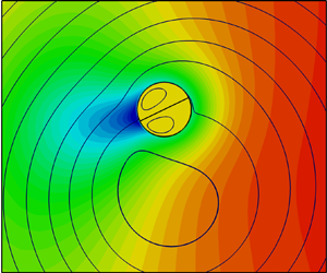
Figure 7. (a) Trajectories of compound drops with different angles  $\alpha$ for $\beta ^1=1, \beta ^2=3$ and $Pe=6$. (b–f) Surfactant distribution and streamlines near the compound drops. The low and high viscosity regions inside the drop are represented by the light-yellow and orange colours, respectively.
Figure 8 shows the average curvature  $\kappa$ of the trajectory and average speed $U$ for drops with fixed $Pe, \beta ^1, \beta ^2$ and different interface angles. It mimics the plot for the oil drop with an evolving phase structure in the experiment (see figure 1). Although the 2-D drop model with a static internal drop phase distribution is significantly different from the 3-D drop in the experiment, our simulation does capture some essential features in figure 1(b). For example, the curvature of the trajectory is non-zero only above a critical value of $\alpha$, above which the curvature has two peaks followed by a gradual decrease. The experiment exhibits a few extra peaks at the late stage of the drop motion. These peaks are related to the drop crossing its own trajectory and cannot be captured by the average curvature in our simulation. The speed of the drop initially decreases with increasing $\alpha$ and then exhibits a large oscillation. Our simulation shows that the speed and curvature are closely correlated with the interior vortices: the speed increases and curvature decreases when the drop has two large interior vortices (figure 7d), and the opposite occurs when the drop forms more vortices with smaller sizes (figure 7c,e). Changing the viscosity inside the drop only quantitatively affects the result. Upon increasing the drop viscosity, the critical angle for the emergence of circular motion increases and the drop speed decreases. In the experiment, the surfactant adsorption rates can be different between the two phases of the drop. To examine this effect, we consider a case with $A^2/A^1=0.5$, assuming that the nematic phase (region 2) creates a smaller concentration gradient than the isotropic phase (region 1) due to its lower FB concentration. The curvature of the drop trajectory in this case is single peaked and it has a higher peak value than the cases with uniform adsorption rates. This shows that the additional source of asymmetry promotes the circular motion. We also note that the curvature of the trajectory is close to the ratio of the average rotational and translational velocities of the drop, i.e. $\kappa \simeq \varOmega /U$. This means that, for a compound drop, its rigid-body rotation is the main cause for the circular motion.

Figure 8. (a) The dependence of the average curvature of the trajectory  $\kappa$ (open symbols and solid lines) and the ratio of average rotation and translation velocities of the drop $\varOmega /U$ (filled symbols and dotted lines) on the intersect angle $\alpha$. (b) The dependence of the average speed $U$ on $\alpha$. The Péclet number of the drop is $Pe=6$, $A^2/A^1=1$ unless otherwise specified.
From the reciprocal theorem, the translational and rotational velocities of a cylindrical swimmer are directly related to integrals of the slip velocity (Elfring Reference Elfring2015)
 $$\begin{gather} U_x=\frac{1}{2{\rm \pi}}\int_0^{2{\rm \pi}}u_\theta|_{r=1}\sin\theta \,{\rm d}\theta,\quad U_y={-}\frac{1}{2{\rm \pi}}\int_0^{2{\rm \pi}}u_\theta|_{r=1}\cos\theta \,{\rm d}\theta, \end{gather}$$
 $$\begin{gather}\varOmega={-}\frac{1}{2{\rm \pi}}\int_0^{2{\rm \pi}}u_\theta|_{r=1} \,{\rm d}\theta. \end{gather}$$
Therefore, the contributions of small vortices with opposite signs tend to cancel each other and result in a lower speed. The curvature in the simulations is systematically lower than that in the experiment, probably due to the differences in surfactant transport and reciprocal relations for two and three dimensions.
In addition to circular motion, compound drops exhibit a strikingly rich variety swimming dynamics for different combinations of  $Pe, \beta ^{1,2}$ and $\alpha$. Figure 9 shows some examples of the drop trajectories found in simulations, including circles, star-shaped circles, quasi-periodic and aperiodic loops, smooth meandering curves, staircase-like zigzag curves and chaotic patterns. These trajectories can be roughly placed into three categories: straight lines, loops and zigzag curves, depending on whether the curvature of the trajectory (or similarly, the angular velocity of the drop) has a preferred sign. Figure 10(a) shows the phase diagram for the three types of trajectories with suggested boundaries for $\beta ^1=1, \beta ^2=3$. In the diagram, the colour shows the mean value of the absolute curvature and the symbol size indicates the drop speed. The categorization of the star-shaped circular trajectories is less definitive than the others. We designate them as loops since their average curvature is typically large, in contrast to the circular trajectories of a single-phase drop. For a drop with two different phases, the trajectory is a straight/zigzag line at small/large $Pe$ when the drop has a dominant phase ( $\alpha \lesssim 0.5{\rm \pi}$ and $\alpha \lesssim 1.7{\rm \pi}$), and the trajectory is generally circular when the two phases are comparable in size, although there are a few exceptions. In figure 10(b) a drop having two phases with the same viscosity shows similar behaviour, except at $\alpha ={\rm \pi}$, when it moves in straight or zigzag lines because of symmetry.

Figure 9. Trajectories of two-phase drops with  $\beta ^1=1$ and different combinations of $Pe, \alpha$ and $\beta ^2$. All plots are shown to scale and the scale bar at the bottom right is 20 times the drop size. Animations of the flow fields around the drops are provided in the supplementary movies available at https://doi.org/10.1017/jfm.2022.891.

Figure 10. The phase diagram of drop trajectories for (a)  $\beta ^1=1, \beta ^2=3$ and (b) $\beta ^1=\beta ^2=1$. Triangle symbols represent zigzag trajectories, and circle symbols represent circular and straight trajectories. The lines mark the approximate boundaries between straight line and circular/zigzag trajectories. The colour shows the average absolute curvature of the trajectory. The symbol size represents the average speed of the drop with larger symbols representing larger speeds.
To understand the transition from straight line to circular/zigzag motion, we proposed a reduced model to analyse the linear stability of the translational motion. At the drop's external surface ( $r=1$), the equation for the surfactant transport is
 \begin{equation} \frac{\partial c}{\partial t}+u_\theta^0\frac{\partial c}{\partial\theta}=\frac{1}{Pe}\frac{\partial^2c}{\partial\theta^2}+f(\theta), \end{equation}
where  $f(\theta )$ is the flux of surfactant to the drop surface due to radial diffusion. We only keep the first two modes of the concentration Fourier expansion, $c=\hat {c}_0+\sum _{k=1}^2(\hat {c}^c_k\cos k\theta -\hat {c}^s_k\sin k\theta )$, where $\hat {c}^c_k$ and $\hat {c}^s_k$ are the real and imaginary parts of $\hat {c}_k$ in (3.14). We assume the tangential velocity on the drop surface has the same terms as a single-phase drop, $u_\theta ^0=-\varOmega +\sum _{k=1}^2(\hat {c}^s_k\cos k\theta +\hat {c}^c_k\sin k\theta )$ (Nagai et al. Reference Nagai, Takabatake, Sumino, Kitahata, Ichikawa and Yoshinaga2013). This simplified model allows us to consider the drop rotation without knowing the detailed information of $f(\theta )$ or the dynamics of the drop. In the base state, the drop moves along its axis of symmetry and the concentration only has even modes. The non-zero coefficients, $\hat {c}^c_k$, which determine the drop speed and surfactant distribution, can be directly solved from (4.4), provided that $f(\theta )$, which should also be an even function of $\theta$, is known. Here, however, we will treat $\hat {c}^c_1$ as an adjustable parameter. From the condition of vanishing velocity at $\theta =\pm ({\alpha }/{2})$, we have the angular velocity $\varOmega =\hat {c}_1^s\cos ({\alpha }/{2})+\hat {c}_2^s\cos \alpha$, the translational velocity $U_x=\tfrac {1}{2}\hat {c}_1^c$ and $U_y=-\tfrac {1}{2}\hat {c}_1^s$, and $\hat {c}_2^c=-\tfrac {1}{2}\hat {c}_1^c\sec ({\alpha }/{2})$. The perturbation equations for $\hat {c}_1^s$ and $\hat {c}_2^s$ can be written as
 \begin{equation} \frac{{\rm d}}{{\rm d}t} \begin{pmatrix} \hat{c}_1^s \\ \hat{c}_2^s \end{pmatrix} =\pmb{\mathbb{A}}\boldsymbol{\cdot} \begin{pmatrix} \hat{c}_1^s \\ \hat{c}_2^s \end{pmatrix}, \end{equation}
where
 \begin{equation} \pmb{\mathbb{A}}= \begin{bmatrix} -\dfrac{1}{Pe}+\left(\cos\dfrac{\alpha}{2}+\dfrac{3}{4}\sec\dfrac{\alpha}{2}\right) \hat{c}_1^c & \left(\dfrac{3}{2}+\cos\alpha\right)\hat{c}_1^c \\ 2\hat{c}_1^c & -\dfrac{4}{Pe}+\cos\alpha\sec\frac{\alpha}{2}\hat{c}_1^c \end{bmatrix}. \end{equation}
Here, we have neglected the perturbations to  $f(\theta )$. The non-rotating drop state is stable when both $\hat {c}_1^s$ and $\hat {c}_2^s$ have negative growth rates, i.e. $\text {Det}(\pmb {\mathbb {A}})>0$ and $\text {Tr}(\pmb {\mathbb {A}})<0$. Otherwise, $\varOmega$ grows exponentially with time and the straight line motion becomes unstable. Figure 11 shows the stability phase diagram in the space of $\alpha$ and $Pe$. The parameter $\hat {c}_1^c$ is a function of $\alpha$ and $Pe$, and its value is estimated to be $|\hat {c}_1^c|\sim 0.1\unicode{x2013}0.4$ based on the range of the simulated drop speed. We set $\hat {c}_1^c$ as a negative constant for $\alpha <{\rm \pi}$, because the drop translates to the negative $x$ direction (figure 7b). For $\alpha >{\rm \pi}$, positive $\hat {c}_1^c$ should be used since the drop moves in the opposite direction (figure 7 f). From (4.6), we can see that the drop rotation is caused by the combined effects of flow stagnation at the interface contact line and the surfactant convection by coupled velocity modes. The analysis predicts that steady translation becomes unstable when $\alpha$ is close to ${\rm \pi}$. The critical $Pe$ for unstable translation decreases as the drop velocity increases. These predictions qualitatively agree with our numerical results.

Figure 11. The stability phase diagram on the space of  $\alpha$ and $Pe$ predicted by the simplified linear stability model for surfactant transport at the drop interface.
It might have been thought that the patterns of the drop trajectories could be distinguished by the eigenvalues with circular trajectories occurring when the eigenvalue is imaginary and zigzag trajectories when the eigenvalue is real. However, our results show that the eigenvalues for the two-mode expansion are real for both types of trajectory. As we will see in the following, the higher-order modes ( $k\geq 3$) are important for the rotational motion of the drop. This also suggests that the nonlinear interaction between drop swimming and surfactant transport plays a critical role in determining the trajectory of the drop.
To compare the circular and zigzag motions, figure 12(a) shows the time history of the angular velocity for the drops with  $\alpha ={\rm \pi}$ and $\beta ^1=3, \beta ^2=3$ at different Péclet numbers. At $Pe=6$ and 10, the drop rotates in the counterclockwise direction, and the high viscosity region of the drop is on the inner side of the circular trajectory. At $Pe=20$ and 30, the drop reverses its rotation moving in clockwise circles with the high viscosity region on the outer side. At an intermediate Péclet number, $Pe=15$, the drop periodically reverses its rotation and moves in a meandering trajectory. In figure 12(b) the distribution of the tangential gradient of surfactant concentration ${\rm d}c/{\rm d}\theta$ and tangential velocity $u_\theta$ on the drop surface look generally similar for all cases. In particular, the lowest concentration (or, equivalently, the largest surface tension), occurs at $\theta \sim 1.6{\rm \pi}$ in the wake region, creating a flow outward from the interface. The maximum and minimum velocities occur at $\theta \sim 1.3{\rm \pi}$ and $\theta \sim 1.9{\rm \pi}$, respectively. The main difference between the fields for drops rotating in different directions appears at $\theta \sim 0.7{\rm \pi}$, where the drop with counterclockwise rotation has a secondary local peak of ${\rm d}c/{\rm d}\theta$ and local minimum of $u_\theta$, representing a new vortex inside the drop. Without this vortex, the drop rotates clockwise because the low viscosity region generates a larger slip velocity than the other side (figure 12c,d). At high Péclet number, the drop speed decreases and the induced flow is not strong enough to advect the surfactant downstream to envelope the drop surface. The accumulation of the surfactant at the front of the drop further decreases the local surface tension and creates a strong slip flow that reverses the drop rotation (figure 12 f). At the intermediate $Pe$, transport of surfactant near the front of the drop regularly switches directions and the flow field shifts between the two states. Therefore, the drop periodically changes its rotation direction and moves in a meandering trajectory.

Figure 12. (a) Time history of the angular velocity of drops at different  $Pe$,
$Pe$,  $\alpha ={\rm \pi}, \beta ^1=1$ and $\beta ^2=3$.(b) Distribution of the tangential gradient of surfactant concentration ${\rm d}c/{\rm d}\theta$ and tangential velocity $u_\theta$ on the drop surface. (c–f) Concentration fields and streamlines near the drops. The red point and arrow show the locations of the lowest surfactant concentration and local peaks of tangential velocity on the drop surface.
Following Li (Reference Li2022), we investigate the correlation between the surfactant concentration and the fluid velocity for different drop swimming motions. Figure 13(a) shows the time history of the magnitudes of the flow modes. For each case, the first two modes have the dominant contribution to the drop swimming. At  $Pe=20$, the stresslet mode ( $k=2$) has a comparable magnitude as the source dipole mode ( $k=1$). It generates a strong extensional flow that changes the surfactant distribution around the drop and induces the extra small vortex inside the drop. At $Pe=15$, the magnitude ratio between the first modes has a large oscillation.

Figure 13. (a) Time history of the magnitude of velocity modes at different  $Pe$,
$Pe$,  $\beta ^1=1, \beta ^2=3$ and $\alpha ={\rm \pi}$. (b–d) The correlation between the surfactant distribution at the drop surface and the orientation of the velocity modes. The results are shown in a drop-fixed frame.
The orientations of the fluid velocity modes changes with  $Pe$ even more than their magnitudes do. Figure 13(b–d) shows the time evolution of the surfactant concentration at the drop surface and the direction of the fluid velocity mode, which for each singularity, is defined by the axis of symmetry of a local converging flow along the drop surface. The results are shown in a drop-fixed frame to reveal the relative angle between the velocity modes and the low concentration wake. The two internal interfaces are located at $\theta ={\rm \pi} /2$ and $3{\rm \pi} /2$ in the plots. When the drop moves in a straight line, all velocity modes align with the axis of symmetry of the concentration wake, creating a pusher-type flow field. In comparison, when the drop moves in a non-straight trajectory, the velocity modes do not align in the same direction. For the drop with $\alpha ={\rm \pi}$, the angular velocity $\varOmega =2\sum _{k=1}(-1)^{k-1}Re[A_{2k}]$ is determined by the even modes ( $k=2,4,6,\ldots$). The ${k=2}$ mode always has a positive angle with respect to the direction of $3{\rm \pi} /2$ and, therefore, has a negative contribution to the angular velocity. In comparison, the orientation of the $k=4$ mode differs at different Péclet numbers. At $Pe=20$, it is on the same side of the internal interface ( $3{\rm \pi} /2$ ) as the $k=2$ mode and causes a positive angular velocity contribution. At $Pe=15$, the $k=4$ mode oscillates and causes a back-and-forth rotation of the drop and, hence, the zigzag motion.
Finally, we examine the run-and-reorient motion for the special case of a drop with two phases having equal volumes and viscosities, i.e.  $\alpha ={\rm \pi}, \beta ^1=\beta ^2=1$. In figure 14(a) the drop moves in a trajectory composed of piecewise segments with a reorientation angle of approximately $102^\circ$. The periodic variation in speed and angular velocity is directly related to the transformations of vortex modes inside the drop. As shown in figure 14(c), the drop forms two vortices inside and swims as a squirmer with an asymmetric slip velocity distribution. The imbalance of the Marangoni stress on the two sides of the drop surface damps the rotation quickly and the drop starts to translate along a straight line with slow rotation ( $\varOmega \sim 10^{-4}$). This motion is unstable due to the emergence of the quadrupole mode, as occurred for the single-phase drop at $Pe\gtrsim 14$ discussed before, and it generates an extra vortex pair in front of the drop. The extra vortex pair gradually transforms the drop into a pusher-type swimmer and reduces the drop speed (figure 14d). The induced flow causes the surfactant to accumulate at the front stagnation point and creates a surface tension gradient that obstructs the drop motion. Eventually in figure 14(e) the translational motion is largely suppressed and the drop creates a symmetric extensional flow field. This flow is intrinsically unstable due to the attraction between two local maxima of surface tension. Outside the drop, the two regions of low surfactant concentration are advected towards each other and merge at a location that is perpendicular to the internal surface, leading to a fast reorientation and slow translation of the drop. After that, the dipole mode gradually outcompetes the quadrupole mode and the drop repeats the translational motion. The formation of the secondary wake of low concentration in front of the drop is biased along the direction of drop rotation, so that it attracts the main wake and causes the reversal of drop rotation in the next cycle.

Figure 14. (a) Trajectory of a drop with equal phase volumes and viscosities  $\alpha ={\rm \pi}, \beta ^1=\beta ^2=1$ and $Pe=15$. Solid and dashed lines are the results simulated using the eigenfunction expansion and finite volume methods for the interior region of the drop, respectively. (b) Time history of the drop speed and angular velocity. (c–e) Concentration field and streamlines near the drop at the time instants marked in (a,b).
Figure 15 shows that the velocity modes for this symmetric drop at  $Pe=15$ change dramatically during the drop motion. The magnitudes of the odd and even modes are strongly anti-correlated: the odd modes have a large magnitude during the drop's translation stage, while the even modes have a large magnitude when the drop slows down and starts to rotate. In the reorientation stage, the formation of the secondary wake of low surfactant concentration only causes the odd modes to change direction. Meanwhile, the even modes remain aligned with the direction of the main wake until they suddenly change direction causing the sudden rotation of the drop. This type of run-and-reorient motion is similar to the meandering motion of a single-phase drop along a trajectory with triangle waves (Li Reference Li2022), but the transition for the two-phase drop is much more abrupt due to the coupling with the drop rotation.

Figure 15. (a) Time history of the magnitude of fluid velocity modes for a drop with  $Pe=15, \alpha ={\rm \pi}, \beta ^1=1$ and $\beta ^2=3$. (b) The correlation between the surfactant distribution at the drop surface and the orientation of the flow velocity modes. The results are shown in a lab-fixed frame.
5. Concluding remarks
To summarize, we have investigated the self-propulsion of a 2-D compound drop composed of two circular sectors driven by Marangoni stresses. Compared with a single-phase drop, the internal interface and viscosity difference introduce more complexity in the hydrodynamic flows and cause a variety of swimming trajectories, including straight lines, circles, smooth and staircase-like zigzag curves, as well as chaotic motions. Depending on whether the trajectory has a predominant bending direction, we classify the trajectories into three categories: straight lines, circles and zigzag curves. Generally speaking, the drop moves in a straight line or zigzag curve when one phase is much larger than the other, whereas its trajectory becomes circular when the two phases are of comparable sizes. The direction of the drop rotation is dependent on the Péclet number. At small  $Pe$, the drop rotates with its high viscosity region on the inner side, and the opposite occurs at high $Pe$. A difference in viscosity of the two phases inside the drop is not necessary for the circular motion. The average speed, on the other hand, is more sensitive to the Péclet number and average viscosity than the size ratio of the two phases. The presence of the internal interfaces reduces the drop speed. For most of the compound drops, the speed scales as $U\sim Pe^{-1/3}$ for $Pe\gtrsim 10$, which is the same as the scaling for a single-phase drop.
Our numerical results can reproduce the key features of experimental observations of a compound oil droplet with continuous phase transformation (Wang et al. Reference Wang, Zhang, Mozaffari, de Pablo and Abbott2021). At relatively low Péclet numbers ( $Pe\lesssim 10$), our study shows the trajectory transforms from straight lines to smooth circles and eventually back to straight lines with increasing volume ratio of the phases. The curvature of the trajectory has a local minimum when the drop has two large interior vortices rather than multiple small vortices. The drop speed reaches a maximum near the conditions for minimal curvature. These results are consistent with the experiments.
At high Péclet numbers, the drop motion exhibits meandering features due to the onset of instability modes at higher wavenumbers, similar to the motion of a single-phase drop. The numerical simulations also discover a run-and-reorient motion for a drop containing two semicircles of equal viscosity at  $Pe\gtrsim 15$. The drop moves along a staircase-like zigzag curve and the flow field inside the drop periodically switches between dipole and quadrupole modes. These results show that the swimming dynamics of the drop is determined by the interplay among various factors: the convection of surfactant around the drop, the distribution of the Marangoni stress on the drop surface, the interior vortices and the difference of flow resistance experienced by the two regions of the drop. The high-order modes play an important role in determining the direction of drop rotation and the pattern of the trajectory.
Several directions can be taken in future research to overcome the limitations of this work. In the current study we use a static drop model to mimic the different stages of a drop with continuous phase transformation. This simplification may partially explain the discrepancies between simulation and experimental results. Transient compositional changes of the drop interior influence the time history of surfactant transport, causing a continuous change in the trajectory curvature in experiment (Wang et al. Reference Wang, Zhang, Mozaffari, de Pablo and Abbott2021). Future simulations could model the changes to the drop interior as one component of the drop is transported into the exterior liquid phase. Secondly, current work uses a fixed flux boundary condition for the surfactant while neglecting the potential for the surfactant to be fully depleted near the drop. This assumption is valid if the concentration variation is small and is useful to focus on the basic physics. However, in practice the drop may completely consume the surfactant, particularly when the drop moves in a small circle. As suggested in our simulation (figure 7a), this effect can reduce the curvature of a circular trajectory and cause an outward spiraling trajectory, similar to the experiment. Finally, 3-D simulations of a compound drop are undoubtedly desirable. Other effects, such as the liquid crystal phase and the deformation of the internal interface can also be important. In the inertial regime the trajectory transition due to vortex shedding (Sur et al. Reference Sur, Masoud and Rothstein2019) can be studied by solving the full Navier–Stokes equations. We also propose that the current simulation may be realized in an experiment using an oil drop floating on the surface of a thin film of surfactant solution (Ichikawa et al. Reference Ichikawa, Takabatake, Miura, Iwaki, Magome and Yoshikawa2013; Pimienta & Antoine Reference Pimienta and Antoine2014). The rotation direction of the compound drops can be easily observed to test the simulation results.
Supplementary movies
Supplementary movies are available at https://doi.org/10.1017/jfm.2022.891.
Acknowledgement
We thank X. Wang and N.L. Abbott at Cornell University for insightful discussions and providing experimental data and animation for figure 1.
Funding
G.L. is Funded by the Scientific Research Staring Foundation (grant no. WH220401009). D.L. Koch acknowledges funding from NSF grant no. 2135617.
Declaration of interests
The authors report no conflict of interest.


 Open access