


1. Introduction
The atmospheric boundary layer (ABL) is the lowest part of the Earth's atmosphere in which we live and breathe. It has been studied numerically by many researchers since the pioneering work of Deardorff (Reference Deardorff1972) concerning an unstable ABL. The ABL is an important example in nature of a wall-bounded turbulent flow. From the evolution of weather and climate patterns to the dispersion of contaminants, the dynamics of the ABL are critical to human activity. One key aspect of the behaviour of the ABL concerns its behaviour at night. During the day, solar radiation warms the surface of the Earth and, under typical sunny conditions, the air's potential temperature decreases with height. At night, however, this effect is reversed and surface cooling leads to the formation of a stably stratified inversion layer which can suppress turbulent motions. Similar suppression of ABL turbulence is seen in winter-time conditions and polar regions. The conditions under which surface cooling can completely or intermittently relaminarize the flow remain the subject of current research.
The meteorology of the stable boundary layer includes states of continuous turbulence and intermittent turbulence (e.g. Businger Reference Businger1973). Mahrt (Reference Mahrt1998) categorized two prototypical states: the weakly stable boundary layer and the very stable boundary layer. The very stable boundary layer is characterized by weak winds and clear skies that lead to strong net radiative cooling at the surface. The weakly stable boundary layer, which has weaker net radiative cooling, is described by Monin–Obukhov similarity theory (Monin Reference Monin1970), in which turbulence, although reduced in strength, occurs continuously in time. On the contrary, the very stable boundary layer is characterized by global intermittency where turbulence is reduced for periods which are long compared with the time scale of individual eddies (Mahrt Reference Mahrt1989). Internal gravity waves are also present in the very stable boundary layer.
The turbulent boundary layer over a rough surface has been reviewed by Raupach, Antonia & Rajagopalan (Reference Raupach, Antonia and Rajagopalan1991) and Jiménez (Reference Jiménez2004), among others. One measure of roughness elements is their height as quantified by a roughness Reynolds number,  $h^+= h/\delta _\nu$, the ratio of the height of the elements to the viscous scale, $\delta _\nu$. With increasing $h^+$, the boundary layer changes from a smooth to a transitionally rough to a fully rough boundary layer. The fully rough boundary layer has enhanced momentum transport and drag. For a given $h^+$, the shape and spatial distribution of the roughness elements are important as reviewed by Flack & Schultz (Reference Flack and Schultz2010) among others. In the present work we consider a periodic array of sinusoidal bumps with moderate slope (figure 1). The analogous problem of unstratified flow over a wavy bottom has received attention in experiments (Zilker, Cook & Hanratty Reference Zilker, Cook and Hanratty1977; Gong, Taylor & Dornbrack Reference Gong, Taylor and Dornbrack1996) and, more recently, in numerical studies using DNS or wall-resolved large-eddy simulation (LES) (e.g. De Angelis, Lombardi & Banerjee Reference De Angelis, Lombardi and Banerjee1997; Sullivan, McWilliams & Moeng Reference Sullivan, McWilliams and Moeng2000; Napoli, Armenio & De Marchis Reference Napoli, Armenio and De Marchis2008; Yang & Shen Reference Yang and Shen2010). Turbulent flow over rough surfaces has a component in the time-averaged field which is coherent with the surface structure and gives rise to a dispersive component of the turbulent fluxes. The coherent velocity can be extracted using a triple decomposition, and the so-called dispersive component is a significant contributor to turbulent fluxes in the near-surface layer (Finnigan Reference Finnigan2000; Sullivan et al. Reference Sullivan, McWilliams and Moeng2000; Poggi, Katul & Anderson Reference Poggi, Katul and Anderson2004; Li & Bou-Zeid Reference Li and Bou-Zeid2019).

Figure 1. Schematic of the computational domain and surface roughness: (a) 2Bump and (b) 4Bump. Here  $L_x, L_y$ and $L_z$ are the domain size in the streamwise, spanwise and vertical directions, respectively. The wavelength of the harmonic function that generates the bump is $\lambda =L_x/N_b$, where $N_b$ is the number of bumps. The half-length of the bump is $l=\lambda /4$.
There is not much systematic study of the competing effects of stable stratification and roughness in canonical problems. Ohya, Neff & Meroney (Reference Ohya, Neff and Meroney1997) and Ohya (Reference Ohya2001) performed laboratory experiments of stratified boundary layers that develop in a wind tunnel over smooth and rough surfaces, respectively. The bottom wall in the rough case had a two-dimensional roughness imposed by a chain of oval rings and had a colder temperature than the bulk flow with  $\Delta \theta$ varying between 27.4 K and 44.1 K. Vertical profiles showed reduction of turbulence levels with increasing stability in both rough and smooth cases. Sullivan & McWilliams (Reference Sullivan and McWilliams2002) conducted DNS of a turbulent Couette flow over waves (including the stationary-wave case) under moderate stable and unstable stratification. Their results show a decrease (increase) of turbulence levels under stable (unstable) stratification.
Turbulence in the boundary layer can collapse in the presence of sufficiently strong stability. Banta et al. (Reference Banta, Mahrt, Vickers, Sun, Balsley, Pichugina and Williams2007) found long periods of suppressed turbulence during nights with a strongly stable ABL. The near-surface layer appears to decouple from the upper regions of the ABL during these episodes of suppressed turbulence. The bulk Richardson number ( $Ri_b$, defined later by (2.11)) is a critical parameter; large values of $Ri_b$ are indicative of strong stability. During periods with $Ri_b >2$ in the cooperative atmosphere–surface exchange study in 1999 (CASES-99) observational campaign, the coupling between the near-surface layer and the outer layer was found to be weak (Poulos et al. Reference Poulos, Blumen, Fritts, Lundquist, Sun, Burns, Nappo, Banta, Newsom and Cuxart2002). Two layers of turbulent kinetic energy (TKE), one above and the other below a local minimum of TKE, were identified by Banta et al. (Reference Banta, Mahrt, Vickers, Sun, Balsley, Pichugina and Williams2007) and Cuxart & Jiménez (Reference Cuxart and Jiménez2007). Such a two-layer configuration of TKE was also found in a recent DNS of the stratified Ekman boundary layer by Gohari & Sarkar (Reference Gohari and Sarkar2018).
The so-called Ekman boundary layer (EBL) is a simplified example of the ABL, whereby a boundary layer in a rotating reference frame develops under unidirectional horizontal flow in geostrophic balance (Coriolis acceleration is equal and opposite to the pressure gradient, both being orthogonal to the flow). The stable EBL is a canonical problem for studying the stabilization of the ABL. Direct numerical simulation studies of the stable EBL have imposed buoyancy with a constant temperature boundary condition (Ansorge & Mellado Reference Ansorge and Mellado2014; Deusebio et al. Reference Deusebio, Brethouwer, Schlatter and Lindborg2014; Shah & Bou-Zeid Reference Shah and Bou-Zeid2014) or with a constant cooling flux (Gohari & Sarkar Reference Gohari and Sarkar2017, Reference Gohari and Sarkar2018); these studies were performed with a smooth-bottom boundary. The boundary-layer response to stability in these studies spanned various regimes of turbulence, depending on the relative strength of the stability: initial decrease of turbulence and even collapse of turbulence to a laminar state; recovery to continuous turbulence; recovery to global intermittency where turbulent near-surface patches co-exist with laminar flow; and, finally, episodes of complete turbulence collapse followed by recovery to spatially intermittent turbulence.
Stratified turbulent channel flow, a canonical problem to investigate buoyancy effects in wall-bounded flows, has received much attention (Garg et al. Reference Garg, Ferziger, Monismith and Koseff2000; Armenio & Sarkar Reference Armenio and Sarkar2002; Nieuwstadt Reference Nieuwstadt2005; Flores & Riley Reference Flores and Riley2011; García-Villalba & del Álamo Reference García-Villalba and del Álamo2011; He & Basu Reference He and Basu2015). Armenio & Sarkar (Reference Armenio and Sarkar2002) show initial collapse of turbulence in a stratified channel flow followed by resurgence of turbulence. They find an outer layer with suppressed turbulence and wavy motion where the gradient Richardson number ( $Ri_g$ defined by (2.8)) is larger than 0.2, and an inner layer with active turbulence where $Ri_g$ decreases from 0.2 to a small value at the wall. García-Villalba & del Álamo (Reference García-Villalba and del Álamo2011), in their large-domain simulations, find global intermittency with laminar patches interspersed within turbulence when the stratification is strong. The surface cooling flux can be used to define the Obukhov length ( $L$, defined later by (2.6)), and its value ( $L^+$, defined later by (2.7)) relative to the viscous scale is an important measure of the strength of buoyancy. Flores & Riley (Reference Flores and Riley2011) propose a criterion for turbulence collapse based on $L^+$ decreasing to 100 during the initial transient. This occurred in their stratified channel with initial $L^+ = 683$.
Coleman, Ferziger & Spalart (Reference Coleman, Ferziger and Spalart1990), Ansorge & Mellado (Reference Ansorge and Mellado2014), Shah & Bou-Zeid (Reference Shah and Bou-Zeid2014), Deusebio et al. (Reference Deusebio, Brethouwer, Schlatter and Lindborg2014) studied the stratified Ekman layer using DNS with a constant temperature imposed at the wall. In this problem the surface buoyancy flux decreases with time although  $Ri_b$ is constant. Intriguing spatial intermittency was observed by Ansorge & Mellado (Reference Ansorge and Mellado2014) in their DNS study of a stably stratified Ekman layer. Similar to Nieuwstadt (Reference Nieuwstadt2005) and Flores & Riley (Reference Flores and Riley2011), initial turbulent collapse followed by recovery was observed when the surface temperature of a neutral Ekman layer was suddenly dropped to impose the prescribed value of stability, $Ri_b$. The spatial characteristics of intermittent turbulence were then analysed in detail during this transient process. In neutrally stratified Ekman layers, Deusebio et al. (Reference Deusebio, Brethouwer, Schlatter and Lindborg2014) found large-scale roll structures with one dominant frequency that matched the convective frequency of the low-level jet (LLJ). They also found that these counter-rotating streamwise vortices influence the near-wall structures by pushing or lifting fluid close to the wall. Shah & Bou-Zeid (Reference Shah and Bou-Zeid2014), from analysis of the TKE budget, show that the reduction of turbulence levels in the stratified EBL is primarily due to the inhibition of shear production rather than the buoyant TKE destruction. Interestingly, this feature of buoyancy-induced reduction of turbulence production, which is key to the suppression of turbulence by density stratification is a generic feature of stratified shear flows and has been found by us in uniform shear flow (Jacobitz, Sarkar & VanAtta Reference Jacobitz, Sarkar and VanAtta1997) and later in the shear layer (Brucker & Sarkar Reference Brucker and Sarkar2007) and the stratified wake (Brucker & Sarkar Reference Brucker and Sarkar2010). The decrease in turbulence production with increasing stratification is an indirect effect of buoyancy that decreases the correlation coefficient between streamwise and vertical velocity fluctuations. Gohari & Sarkar (Reference Gohari and Sarkar2017) performed DNS of the Ekman layer with a constant buoyancy flux, and found differences of this constant-flux stability case with respect to previous cases with constant temperature stability: the low-level jet is stronger, there are recurring episodes of collapse and rebirth of turbulence during the transient, and the TKE profile has local peaks at two vertical locations.
Recently, Gohari & Sarkar (Reference Gohari and Sarkar2018) conducted DNS of a smooth-surface EBL that is subject to a finite-time (approximately, one inertial period) cooling flux. They found that initial  $L^+_{cri}=Lu^*/\nu \lesssim 700$ provides a cooling flux that is sufficiently strong to cause the initial collapse of turbulence independent of Reynolds number, $Re_*$, where $L$ is the Obukhov length scale and $u^*$ is the friction velocity. The turbulence collapse criterion for stratified Ekman flow is considered based on the normalized Obukhov length scale (Obukhov Reference Obukhov1971), $L^+$, and has similar values as inferred from the observational study of Banta et al. (Reference Banta, Mahrt, Vickers, Sun, Balsley, Pichugina and Williams2007) and the DNS of Flores & Riley (Reference Flores and Riley2011). The final state, for a fixed $L^+$ and a fixed cooling flux, was found to depend on $Re_*$, because an increase in initial $Re_*$ (under the constraint of fixed $L^+$) is equivalent to an increase in $Ri_b$. In particular, an EBL with a final stability of $Ri_{b} \geq 2$ relaminarized.
None of the Ekman layer DNS have considered surface roughness, which is often a feature of the ABL. This motivates the present research that addresses how the destabilizing effect of surface roughness competes with the stabilizing effect of surface cooling in the EBL. The simulation results are related to meteorological characteristics that are distinctive features of the stable ABL: low-level jets (Smedman, Tjernström & Högström Reference Smedman, Tjernström and Högström1993; Cuxart et al. Reference Cuxart, Yagüe, Morales, Terradellas, Orbe, Calvo, Fernández, Soler, Infante and Buenestado2000; Banta et al. Reference Banta, Newsom, Lundquist, Pichugina, Coulter and Mahrt2002), collapse of surface-layer turbulence (Banta et al. Reference Banta, Mahrt, Vickers, Sun, Balsley, Pichugina and Williams2007), local turbulence peaks at locations above the surface layer (Mahrt Reference Mahrt1985; Smedman et al. Reference Smedman, Tjernström and Högström1993; Banta et al. Reference Banta, Mahrt, Vickers, Sun, Balsley, Pichugina and Williams2007) and unsteadiness of turbulence statistics (Banta Reference Banta2008; Pichugina et al. Reference Pichugina, Tucker, Banta, Brewer, Kelley, Jonkman and Newsom2008; Sun et al. Reference Sun, Mahrt, Banta and Pichugina2012). These characteristics not only change the atmospheric dispersion of tracers and pollutants, as has been well documented in the past, but also, as discussed in recent work, strongly influence acoustic propagation in the nocturnal boundary layer (Talmadge et al. Reference Talmadge, Waxler, Xiao, Gilbert and Kulichkov2008) with this influence being modified by hilly terrain (Damiens, Millet & Lott Reference Damiens, Millet and Lott2018).
The work is organized as follows. Section 2 describes the governing equations and the problem set-up. Section 3 describes the results of the simulations through the evolution of mean and turbulence statistics. Section 4 describes the flow structures by isosurface visualizations and elucidates the role of coherent structures by a triple decomposition. Finally, § 5 contains the discussion and conclusions.
2. Formulation
In the study of the stratified EBL, several important physical parameters arise: the geostrophic wind  $U_\infty$, the Coriolis frequency $f$, the turbulent Ekman layer thickness $\delta _*$ and the friction Reynolds number $Re_*$. The governing equations for the conservation of momentum under the Boussinesq approximation and potential temperature in a rotating reference frame are as follows:
 \begin{gather} \frac{\partial{u}_i}{\partial t}+ \frac{\partial({u}_i{u}_j)}{\partial x_j}=-\frac{\partial{p}}{\partial x_i}+\nu{\nabla^2} u_i +\delta_{i3}\beta g {\theta} +f\epsilon_{ij3}({u}_j-U_{\infty}\delta_{j1}), \end{gather}
 \begin{gather}\frac{\partial{\theta}}{\partial t}+ \frac{\partial({\theta}{u}_j)}{\partial x_j}=\alpha\nabla^2 \theta . \end{gather}
Here  $t$ is time, $x_{j}$ is the spatial coordinate in the $j$ direction, $u_j$ is the velocity component in that direction, $p$ is the pressure deviation from the mean pressure imposed by geostrophic and hydrostatic balance, $\delta _{i3}$ is the Kronecker delta, $\epsilon _{ij3}$ is the alternating unit tensor, $\nu$ is the molecular viscosity, $\beta$ is the thermal expansion coefficient for air, $g$ is the gravitational acceleration, $f$ is the Coriolis parameter, $\alpha$ is the thermal diffusivity and $\theta$ is the deviation of potential temperature from its constant reference value.
It can be shown that Reynolds number and Prandtl number, defined as
 \begin{equation} Re_D=\frac{U_{\infty}D}{\nu},\quad D=\sqrt{2\nu/f} , \quad Pr=\frac{\nu}{\alpha} , \end{equation}
are the only non-dimensional parameters controlling the dynamics of a neutral Ekman flow at steady state, when the statistics have been adequately decorrelated from their initial condition (Spalart Reference Spalart1988). Although the laminar Ekman layer depth,  $D$, is not a proper length scale describing the momentum transport in a turbulent Ekman flow, $Re_D$ provides a universal comparison point among different Ekman flow studies. For a turbulent Ekman flow, it is proper to use the turbulent Ekman layer thickness, $\delta _N = u_{*}/f$, where $u_*$ is the friction velocity which is defined below and subscript $N$ denotes neutral conditions. The friction velocity and the friction Reynolds number ( $Re_*$) are computed as
 \begin{equation} \left. \begin{array}{c@{}} u_*^2 =\displaystyle \nu \left.\sqrt{ \left( \dfrac{ \partial {\langle {u} \rangle}}{\partial z} \right)^2+ \left( \dfrac{\partial {\langle {v} \rangle}}{\partial z} \right)^2 } \right|_{z=0},\\ Re_* = \displaystyle\dfrac{u_*\delta_N}{\nu}. \end{array} \right\} \end{equation}
Hereafter,  $\langle \cdot \rangle$ denotes the Reynolds average, which is computed as a horizontal $x$–
$x$– $y$ average when the flow statistics are evolving in time, and with an additional time average over an inertial period when the flow is quasi-steady. It is important to note that $u_*$ and $\delta _N$ are functions of the Reynolds number and are not known prior to simulation in Ekman layer studies. Denoted by superscript $+$, statistics normalized with the viscous scale ( $\nu /u_*$) are chosen to describe behaviour in the near-surface region. Normalization of statistics, denoted by superscript $-$, by the boundary-layer height (Ekman layer thickness $\delta _N$) is also used.
2.1. Surface roughness
The roughness takes the form of periodic two-dimensional periodic bumps whose non-dimensional amplitude is fixed and the steepness is changed among cases. The rough surface is described by a height function,  $\eta (x)$, which is generated through a harmonic function, $f(x) = - h \cos (2{\rm \pi} x/\lambda )$, with wavelength $\lambda$ and amplitude $h$, including only the positive portions of $f(x)$,
 \begin{equation} \eta(x) = \begin{cases} f(x) & \text{if } f(x)= - h \cos (2{\rm \pi} x / \lambda) >0,\\ 0 & \text{otherwise}. \end{cases}\end{equation}
 A schematic of the roughness (figure 1) shows the surface has bumps but, unlike a surface wave, it has no troughs. This choice is motivated by the example of a two-dimensional hilly surface. Other types of surface roughness, e.g. a wavy surface that has been studied in the past, are worth future consideration. The chosen roughness has not only a small height ( $h^+ =15$) relative to the Ekman layer thickness but also has a gentle slope ( $h/\lambda \ll 1$), so that, in the unstratified cases, its effect is small. In the stratified cases, as will be shown and explained, the same roughness height has a strong effect that substantially changes the flow with respect to its smooth-bottom counterpart. The influence of roughness is found to extend up to the region ( $Ri_g > 0.1$) where buoyancy alters the mean flow and turbulent stresses.
2.2. Buoyancy
Buoyancy is imposed by a surface flux, whose strength is quantified by the Obukhov length,
 \begin{equation} L=-\frac{u_*^3}{\kappa (\beta g q_0)},\end{equation}
where  $\kappa$ is the von-Kármán constant and $q_0=-\alpha \partial _z \theta |_{z=0}$ is the applied surface cooling flux. Here $L$ provides an estimate of the height at which the buoyancy flux and turbulent energy production by mean shear are balanced. Using inner-layer scaling, the normalized Obukhov length becomes
 \begin{equation} L^+ = \frac{L u_*}{\nu}=-\frac{u_*^4}{\kappa \nu (\beta g q_0)}.\end{equation}
The gradient Richardson number, a function of  $z$ and $t$ in this flow, is defined by
 \begin{equation} Ri_{g}=\frac{N^2}{S^2},\end{equation}
where  $N^2 = g\beta \partial {\langle \theta \rangle }/\partial z$ is the squared buoyancy frequency and $S^2=(\partial {\langle u \rangle }/\partial z)^2+(\partial {\langle v \rangle }/\partial z)^2$ is the squared mean of the vertical shear. Large local values of $Ri_g$ imply suppression of shear production of turbulence, and $Ri_g = 0.25$ is a stability boundary for the stratified shear layer. The non-dimensional inverse Obukhov length scale can also be interpreted in terms of $Ri_g$ at the surface,
 \begin{equation} Ri_{g,s}=\frac{N^2}{S^2}=\frac{\beta g \partial_{z}\langle \theta_0 \rangle}{{u_*^4}/\nu^2}=(\kappa L^+)^{-1}, \end{equation}
where  $Pr = 1$ has been assumed. An alternative normalization of $L$ is based on outer-layer coordinates,
 \begin{equation} L^- = \frac{L}{\delta_N},\end{equation}
where  $\delta _N = u_{*}/f$ is the boundary-layer scale. The neutral EBL has a boundary-layer height of approximately $0.5 \delta _N$. Since $u_*$ is a time-dependent function in the stratified DNS cases, so are $L, L^+$ and $L^-$.
The bulk Richardson number, an overall stability measure of the flow, is defined as
 \begin{equation} Ri_b =\beta g\delta_N\frac{\langle\Delta \theta_0 \rangle}{U_\infty^2},\end{equation}
where  $\Delta \theta _0=\theta _\infty -\theta _0$ is the difference between the temperature above the boundary layer and the surface temperature. In the present study the surface temperature ( $\theta _0$) is a time-dependent variable during the time interval, $T$, over which finite-time constant-flux stability is imposed. The value of $Ri_b$ is also initially dependent on time but it becomes constant at the end of the time interval, $T$.
$T$.
2.3. Numerical details
The governing equations (2.1) and (2.2) are numerically advanced in time using a combination of the low-storage third-order Runge–Kutta (RKW3) and mixed spectral-physical spatial discretization. The equations are written in generalized coordinates and the grid conforms to the bottom wall as described by Gayen & Sarkar (Reference Gayen and Sarkar2011). Spatial discretization and derivative calculations in the spanwise direction are performed using Fourier transforms, and the derivatives in the streamwise and vertical directions are computed using a second-order central difference scheme. The nonlinear advection terms are dealiased with the 2/3 rule and a sharp-cutoff filter. The kinematic pressure,  $p$, is computed by solving the Poisson equation that results from imposing zero velocity divergence at each time step. The boundary conditions for the velocity are no-slip and impermeability ( $u_i=0$) at the surface, periodicity in the horizontal directions and stress free ( $\partial u_i/\partial z=0$) at the upper boundary. The temperature gradient is fixed at the bottom surface to impose the desired cooling flux. A sponge region with Rayleigh damping is applied to $u_i$ and $\theta$ to minimize the spurious reflection of gravity waves in the upper boundary ( $z=L_z$). The in-house solver, which has been developed for environmental flows, has been applied to the Ekman boundary layer (Gohari & Sarkar Reference Gohari and Sarkar2018) as well as complex geometries including stratified oscillating flow over a slope (Gayen & Sarkar Reference Gayen and Sarkar2011) and a triangular ridge (Rapaka, Gayen & Sarkar Reference Rapaka, Gayen and Sarkar2013; Jalali, Rapaka & Sarkar Reference Jalali, Rapaka and Sarkar2014).
A cooling flux, as determined by  $L^+$, is imposed in the neutral cases too in order to simulate the behaviour of a passive scalar. All of the rough and smooth-bottom stratified cases are initiated with a fully developed velocity field taken from the corresponding neutral case. The passive-scalar temperature field from the neutral case is reset to a uniform background value so that each stratified case starts with zero temperature variation and stratification is allowed to build up in response to the applied surface buoyancy flux.
Parameters used in this DNS study are summarized in table 1. A fixed value of buoyancy flux, corresponding to  $L^+{\approx 700}$, is applied for a time interval of $f\,T = 6$ in the stable cases. Note that the computational domain is enlarged to twice the streamwise domain of Gohari & Sarkar (Reference Gohari and Sarkar2018) in order to better accommodate long streamwise structures. The resolution is $\Delta x^+ \approx 8.5$ in the streamwise direction for the flat-bottom case and $\Delta y^+ \approx 5.2$ in the spanwise direction, similar to other DNS of wall-bounded flows. For the rough cases, the resolution in the streamwise direction is increased to $\Delta x^+ \approx 5.6$. In the vertical direction, ten grid points span $0 < z^+ \leq 10$ with a non-dimensional grid spacing $\Delta {z}_{min}^+ \leq 1$.
Table 1. Physical and numerical parameters of the simulations. Here  $N_x, N_y$ and $N_z$ are the number of grid points in the streamwise, spanwise and vertical directions, respectively. The case label in column 1 has a subscript $N$ (neutral case) or $S$ (stable case), and starts with the number of bumps in the rough cases. In the stable cases, a surface buoyancy flux, chosen to obtain a target $L^+\approx 700$, is applied for a finite time of $f\,T \approx 6$ and then the surface temperature is held constant.

The roughness height is kept constant at a small value of  $h^+ = 15$ which corresponds to the transitionally rough regime. The roughness takes the form of a periodic array of two-dimensional, spanwise-uniform elements whose surface elevation is given by (2.5). The roughness amplitude, $h^+ =15$, is kept constant, and the wavelength of the roughness ( $\lambda$) is changed. Note that $\lambda =L_x/N_b$, where $N_b$ is the number of bumps and $L_x$ is the streamwise domain size. In the simulations $L_x$ is kept fixed and $\lambda$ is changed by changing $N_b$. Doubling $N_b$ decreases the element half-length ( $l = \lambda /4$) by a factor of 2 and doubles the slope. The coverage of the bottom by the roughness elements is 50 % of the wall area, independent of the number of bumps. The slope of each bump, given by $h/l$, is small and changes from 0.042 to 0.084 when $N_b$ is doubled from 2 to 4. Another measure is the maximum slope, $hk$ where $k= 2{\rm \pi} /\lambda$ is the wavenumber, which changes from 0.06 to 0.12. We find that the flow does not separate at these values of slope. It is worth noting that the slope utilized here is below the critical slope for separation reported in the literature on a sinusoidal wavy surface where Gong et al. (Reference Gong, Taylor and Dornbrack1996), Sullivan et al. (Reference Sullivan, McWilliams and Moeng2000) quote ${hk > 0.3}$ for flow separation, and Zilker et al. (Reference Zilker, Cook and Hanratty1977) state that there is incipient separation at $2h/\lambda = 0.05$ and there are large separated regions at $2h/\lambda = 0.125$ and 0.20.
3. Flow evolution
The effect of the small-amplitude bumps on the velocity and temperature profiles in  $z$ is found to be insignificant under neutral conditions in contrast to the substantial effect under stratified conditions. This primary result is elaborated and explained in this section.
3.1. Overall velocity and temperature variation
Figure 2 shows the horizontal mean velocity ( $\sqrt {\langle u \rangle ^2+\langle v \rangle ^2}/U_{\infty }$) profile of the EBL in the top row and the normalized potential temperature ( $u_{*_N} (\theta - \theta _{\infty })/q_0$) in the bottom row for both neutral (left column) and stratified (right column) cases. The statistics are obtained by averaging over the horizontal $x$–
$x$– $y$ plane and an average over one inertial period ( ${\,ft \approx 2{\rm \pi}}$). The temperature is treated as a passive scalar in the neutral cases. The velocity in the neutral flat-bottom case compares well with previous results (Shingai & Kawamura Reference Shingai and Kawamura2004; Ansorge & Mellado Reference Ansorge and Mellado2014; Shah & Bou-Zeid Reference Shah and Bou-Zeid2014) at comparable $Re$ as discussed by Gohari & Sarkar (Reference Gohari and Sarkar2018). The horizontal wind speed exhibits little difference among the neutral (figure 2a) flat and rough cases. Since the slope of the bump is gentle ( $hk = 0.06$ and 0.12), the flow does not separate and the change in wall drag (shear stress plus form drag) is small. It is worth noting that DNS of a turbulent flow over a sinusoidal wavy wall with $hk = 0.1$ in Couette flow (Sullivan et al. Reference Sullivan, McWilliams and Moeng2000) and channel flow (De Angelis et al. Reference De Angelis, Lombardi and Banerjee1997) does not show flow separation. The stratified cases also do not exhibit flow separation; however, the mean velocity profiles (figure 2b) show a strong influence of roughness on the features of the LLJ that forms in the boundary layer. Each stratified case has a super-geostrophic velocity, commonly referred to as the LLJ. The formation of the LLJ is a distinctive feature of the stable ABL (Beare et al. Reference Beare, Macvean, Holtslag, Cuxart, Esau, Golaz, Jimenez, Khairoutdinov, Kosovic and Lewellen2006) associated with the reduction of turbulent momentum flux by buoyancy. In the roughness layer at the surface, the bumps counteract the buoyancy-induced reduction of the momentum fluxes. Thus, the peak of the LLJ moves upward and the LLJ profile broadens. In the stratified 4Bump case (filled diamonds in figure 2b), the wind-speed profile in the region between the surface and $z^- = 0.1$ is close to the neutral case (open diamonds) while, in contrast, the 2Bump and flat cases exhibit a significant deviation from the neutral case. The present DNS results show a LLJ with a nose at $z\approx 0.1 \delta _N$, with a maximum super-geostrophic overshoot of $u/u_\infty -1\approx 10\,\%$. Direct numerical simulation with stronger stability conducted by Gohari & Sarkar (Reference Gohari and Sarkar2017) showed cases with LLJ at $z\approx 0.05 \delta _N$ and $u/u_\infty -1\approx 50\,\%.$ Considering typical values of $u_* \approx 0.3$ m s $^{-1}$ and $f=10^{-4}$ s $^{-1}$ in the DNS-derived scaling gives a LLJ nose height of 150–300 m in the stable ABL. This estimate of LLJ properties is consistent with several stable ABL studies: (i) Banta et al. (Reference Banta, Mahrt, Vickers, Sun, Balsley, Pichugina and Williams2007) reported LLJ nose height at approximately 150–300 m with velocity overshoot of 20–60 %; (ii) Beare et al. (Reference Beare, Macvean, Holtslag, Cuxart, Esau, Golaz, Jimenez, Khairoutdinov, Kosovic and Lewellen2006) reported LLJ nose height at approximately 150–180 m with an overshoot of 25 % in LES studies; (iii) Banta et al. (Reference Banta, Newsom, Lundquist, Pichugina, Coulter and Mahrt2002) reported LLJ nose height at approximately 100–200 m with a velocity overshoot of 10–70 %; (iv) Talmadge et al. (Reference Talmadge, Waxler, Xiao, Gilbert and Kulichkov2008) reported observations of LLJ nose height at approximately 125 m in an ABL with strong ground cooling (see figure 4 in Talmadge et al. Reference Talmadge, Waxler, Xiao, Gilbert and Kulichkov2008); (v) Wilson, Noble & Coleman (Reference Wilson, Noble and Coleman2003) studied sound propagation in a stable nocturnal boundary layer which had a deep temperature inversion and LLJ at approximately 160 m, and was observed during CASES-99 (Poulos et al. Reference Poulos, Blumen, Fritts, Lundquist, Sun, Burns, Nappo, Banta, Newsom and Cuxart2002). It is worth noting that sloping terrain that leads to drainage flows also contributes to the LLJ structure (Mahrt Reference Mahrt1999).

Figure 2. Mean velocity ( $\sqrt {\langle u \rangle ^2+\langle v \rangle ^2}/U_{\infty }$) profiles: (a) neutral and (b) stratified cases. Potential temperature ( $u_{*_N}(\theta - \theta _{\infty })/q_0$) profiles: (c) neutral cases where $\theta$ is treated as a passive scalar, and (d) stratified cases. The large unfilled circle (right column) marks the time-evolving boundary-layer thickness ( $z = \delta _t$), defined by (3.7a,b).
In the neutral EBL (figure 2a) the effect of the surface roughness on the mean temperature is relatively small, similar to that on the velocity. However, in the stratified boundary layer (figure 2b) the bumps have a significant effect on the temperature distribution. The strong near-surface inversion of the flat case is substantially weakened in the 4Bump case; the near-surface temperature field is more mixed, and its profile moves towards that of the neutral case. Thus, in spite of employing the identical value of surface cooling flux ( $q_0$) in the three stratified cases, the surface temperature in the 4Bump case does not decrease as much as in the other stratified cases.
The mean velocity is also examined using inner-layer coordinates. A least-squares fit to the vertical variation of  $G = (\langle u\rangle ^2 + \langle v\rangle ^2)^{1/2}$ is performed to obtain the following profile in semi-logarithmic coordinates:
 \begin{equation} G^+=\frac{1}{\kappa}\ln{z^+} + B \equiv \frac{1}{\kappa}\ln{\frac{z^+}{{z_0}^+}}\equiv \frac{1}{\kappa}\ln{\frac{z}{{z_0}}}.\end{equation}
Here  ${z_0}^+=e^{-\kappa B}$. The values of ( $\kappa , {z_0}^+$) are (0.44, 0.0759), (0.43, 0.0814) and (0.40, 0.1187) in the flat, 2Bump and 4Bump cases, respectively, and the profiles are as shown in figure 3. Sullivan et al. (Reference Sullivan, McWilliams and Moeng2000) in their DNS of Couette flow found that, for a stationary bottom wall, ${z_0}^+ = 0.17$ in the flat-bottom case and ${z_0}^+ = 0.27$ for a wavy-bottom wall with $ak= 0.1$. Both cases exhibited $\kappa = 0.41$.

Figure 3. The mean velocity magnitude plotted in semi-logarithmic coordinates: (a) flat  $\kappa = 0.44, \ B = 5.82, \ z_{0} = 0.0759$, (b) 2Bump $ \kappa = 0.43, \ B = 5.77, \ z_{0} = 0.0814$, and (c) 4Bump $ \kappa = 0.40, \ B = 5.32, \ z_{0} = 0.1187$.
Monin–Obukhov (MO) similarity theory, often used to interpret ABL data, is utilized to assess the mean velocity and temperature profiles obtained here. Simulation data are used to compute stability functions ( $\varPhi _m$ and $\varPhi _h$) associated with MO similarity theory:
 \begin{equation} \varPhi_m = \kappa z \dfrac{\sqrt{\left(\dfrac{\partial {\langle {u} \rangle}}{\partial z}(z)\right)^2+\left(\dfrac{\partial {\langle {v} \rangle}}{\partial z}(z)\right)^2}}{u_*(z)}, \quad \varPhi_h = -\kappa z \dfrac{\dfrac{\partial {\langle {\theta} \rangle}}{\partial z}(z)}{\theta_*(z)}. \end{equation}
Here  $u_*(z)$ and $\theta _*(z)$ are the local scales for velocity and temperature fluctuations, as per local similarity theory (Nieuwstadt Reference Nieuwstadt1984):
 \begin{gather} u_*(z)^2 = \nu\sqrt{\left( \frac{\partial {\langle {u} \rangle}}{\partial z}(z) \right)^2+ \left(\frac{\partial {\langle {v} \rangle}}{\partial z}(z) \right)^2} + \sqrt{ { \langle u'w' \rangle}^2 + {\langle v'w' \rangle}^2}, \end{gather}
 \begin{gather}\theta_*(z)u_*(z) = {\alpha} \frac{\partial {\langle {\theta} \rangle}}{\partial z}(z) + {\langle \theta'w' \rangle}, \end{gather}
 \begin{gather}L_L(z)=-\frac{u_*(z)^3}{\kappa ({\beta} g q_0)}. \end{gather}
In the unstratified cases,  $\varPhi _h$ is computed using passive-scalar statistics (buoyancy term in the momentum equation is set to zero) and the computed value of $L_L$ is to be understood as a notional value that allows comparison of profiles with the stratified cases.
Figure 4 shows normalized mean gradients (the so-called stability functions) for unstratified (a,b) and stratified (c,d) Ekman layers. For the unstratified cases,  $\varPhi _m (z) = 1$ is expected in the log-law region and, correspondingly, $\varPhi _m (z)$ takes values near unity over an extended region (figure 4a). Very near the bottom and in the roughness sublayer, $\varPhi _m (z)$ increases with increasing $z$. According to MO theory, $\varPhi _m$ and $\varPhi _h$ are constant and close to unity when $z/L_L \ll 1$; here $L_L$ is the local Obukhov length. When $z/L_L \geq O(1)$, the turbulent length scale becomes limited by the local Obukhov length and $\varPhi _m (z)$ increases with $z$. As shown in figure 4(c,d), there is a region, $0.02 < z/L_L < 0.1$, where $\varPhi _m$ is approximately constant but greater than unity, followed by an increase of $\varPhi _m$ as a function of increasing $z/L_L$ . The function $\varPhi _h (z)$ also increases with increasing $z/L_L$ and exhibits a slope that is larger than that of $\varPhi _m (z)$. Thus, the effect of buoyancy on heat transport is stronger than on momentum transport, i.e. the turbulent Prandtl number becomes larger than 1 in the stratified region of the boundary layer. The dependence of the stability functions on $z/L_L$ in the present work is similar to that reported in previous studies, e.g. the LES of Basu & Porté-Agel (Reference Basu and Porté-Agel2006). It is worth noting that, in the surface layer and among the stratified cases, the 4Bump case shows behaviour closest to the passive-scalar counterpart.

Figure 4. Normalized gradients ( $\varPhi _m$ and $\varPhi _h$ defined by (3.2a,b)) of velocity (a,c) and temperature (b,d). Passive-scalar, unstratified cases are shown in the top row (a,b) and stratified cases in the bottom row (c,d).
Figure 5 shows the overall influence of the bumps on the flow evolution. The integrated TKE, obtained by a horizontal  $x$–
$x$– $y$ average to compute $\langle u_i'u_i'\rangle$ followed by integration in the vertical, is defined as
 \begin{equation} E=\int e \, \textrm{d} z=\tfrac{1}{2}\int_{0}^{L_z} \langle u_i'u_i'\rangle \, \textrm{d} z. \end{equation}
Figure 5. Overall behaviour of the stratified cases at  $Re_* \approx 700$: (a,b) flat cases, (c,d) 2Bump cases and (e,f) 4Bump cases. The left column shows integrated TKE ( $E/(\delta _N {u^2_{*_N}})$) and the right column shows the bulk Richardson number ( $Ri_b$). Points a–f (left column) mark the times of (a–f) in figure 7.
In all cases, TKE initially decreases during a period of turbulence collapse when the flow transitions from neutral to stable. For the flat case, turbulence collapses with a time scale of  $L/u_*$ in agreement with Flores & Riley (Reference Flores and Riley2011). The collapse is followed by a recovery of TKE in each case. The turbulence recovery is consistent with DNS results of the stable EBL (Ansorge & Mellado Reference Ansorge and Mellado2014; Shah & Bou-Zeid Reference Shah and Bou-Zeid2014; Gohari & Sarkar Reference Gohari and Sarkar2018). The value of $u_*$ decreases by $\sim$10–15 % during the initial transient before recovering to approximately its initial value. In an analysis of the CASES-99 data, Banta et al. (Reference Banta, Mahrt, Vickers, Sun, Balsley, Pichugina and Williams2007) reported a 6 hr collapse time period which corresponds to a non-dimensional time of ${ft\approx 1.98}$, which is similar to the DNS collapse time scale.
The TKE evolution after collapse exhibits significant differences among cases. In figure 5(a,c) for the flat and 2Bump cases, TKE exhibits a large-amplitude inertial oscillation with period,  $ft \approx 2 {\rm \pi}$. For the 4Bump case (figure 5e), the periodic modulation of TKE is not observed, but TKE exhibits a gradual increase (on average) and seems to reach a plateau beyond $ft \approx 25$. We will discuss reasons for the difference in TKE evolution later.
We apply the same buoyancy flux for all cases; however, the final  $Ri_b$ (right column of figure 5) is different among the three cases. The final value of $Ri_b$ for the flat, 2Bump and 4Bump cases is 0.485, 0.379 and 0.312, respectively. Thus, the modification of the flow by the roughness elements is sufficiently strong in the 4Bumps case, despite the small bump height and the gentle slope of the bump, to significantly decrease $Ri_b$. The decrease in $Ri_b$ suggests that the buoyancy effect in the 4Bump case on turbulence is weaker, as will be demonstrated by quantification of turbulent fluxes.
The contour of local gradient Richardson number,  $Ri_g$ defined by (2.8), is a measure of the height-dependent strength of static stability relative to shear instability, and is depicted in figure 6. There is a region extending up from the wall which is subcritical ( $Ri_g < 0.25$). The height at which $Ri_g$ crosses the critical value of 0.25 increases with the number of bumps so that the subcritical region of the $Ri_g$ profile expands significantly. The subcritical region that starts at the bottom reaches up to $z^- \approx 0.2$ in the 4Bump case instead of $z^- \approx 0.075$ in the flat case. The implication is that roughness changes the stability of the near-bottom flow to make it more vulnerable to shear instability. Thus, the behaviour of both $Ri_b$ and $Ri_g(z)$ suggest that the roughness elements, albeit small, substantially mitigate the stabilizing effect of buoyancy.

Figure 6. Contours of gradient Richardson number ( $Ri_g$) for flat (a), 2Bump (b) and 4Bump (c) cases. The black dashed line shows $Ri_g=0.25$.
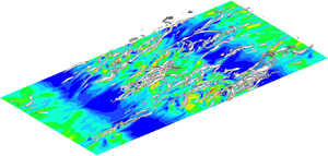
In figure 7 instantaneous vertical vorticity contours for the three stratified cases at different times ( $ft \approx {\rm \pi}$ in the left column and $ft \approx 4 {\rm \pi}$ in the right column) are shown on a horizontal plane close to the wall ( $z^+ \approx 16$) and near the crest of the bumps. These times correspond to points (a–f) on the TKE profiles shown in the left column of figure 5 and also to panels (a–f) in figure 7. Comparison of the points demarcated as b, d and f on the time histories in figure 5 show that, at $ft \approx 4{\rm \pi}$, the integrated TKE is the same for 2Bump and 4Bump cases and is slightly smaller in the flat case. However, on comparison of figures 7(b), 7(d) and 7(f), we find that the near-wall structures are substantially different, reinforcing the fact that an overall statistical measure of turbulence does not necessarily reveal the full picture of the flow state. In particular, with an increasing number of bumps, near-wall turbulence is less patchy and more continuous at $ft = 4 {\rm \pi}$, corresponding to a state of continuous turbulence without global intermittency (Nieuwstadt Reference Nieuwstadt1984). This is true even at the earlier time of $ft = {\rm \pi}$ during the initial adjustment of the boundary layer to buoyancy when the TKE drops.

Figure 7. Vertical vorticity (normalized with  ${u_*}_N/z$) contour at $z^+ \approx 16$ in the stratified cases: (a,b) flat, (c,d) 2Bump and (e,f) 4Bump. Left column at $ft \approx {\rm \pi}$ and right column at $ft \approx 4 {\rm \pi}$.
3.2. Boundary layer thickness
Previous studies have chosen different metrics to quantify the thickness of the stratified boundary layers, including but not limited to the height of the capping inversion layer (Melgarejo & Deardorff Reference Melgarejo and Deardorff1974; André & Mahrt Reference André and Mahrt1982), the height at which the low-level jet velocity is maximum (Blackadar Reference Blackadar1957; Shapiro & Fedorovich Reference Shapiro and Fedorovich2010; Van de Wiel et al. Reference Van de Wiel, Moene, Steeneveld, Baas, Bosveld and Holtslag2010), and the height at which turbulent stress reduces to some fraction of its surface value (Zilitinkevich Reference Zilitinkevich1972; Businger & Arya Reference Businger and Arya1975; André & Mahrt Reference André and Mahrt1982; Kosović & Curry Reference Kosović and Curry2000). Although each of these definitions has a suitable use, the one defined based on the location where turbulent stress vanishes is chosen here as an average measure of the interface between turbulent and non-turbulent layers. We define the height by locating the position (denoted by  $z_p$) where the horizontal Reynolds shear stress is reduced to 5 % of $u_*^2$, and then linearly extrapolating to the location at which it would vanish if the stress profile was linear. Thus, a time-evolving value of the stratified boundary-layer thickness is defined as
 \begin{equation} \delta_t = \frac{z_p}{0.95};\quad \textrm{at}\ z = z_p, \quad \sqrt{\langle u'w' \rangle^2 +\langle v'w' \rangle^2}/u_{*}^2=0.05. \end{equation}
Subsequently, a modified bulk Richardson number, based on the local (in time) boundary-layer thickness, is defined as
 \begin{equation} Ri_{b,t} =\beta g\delta_t\frac{\langle\Delta \theta_0 \rangle}{U_\infty^2}.\end{equation}
 Figure 8(a) shows the time evolution of  $\delta _t$ for the stratified cases. In the flat case, the EBL thickness decreases sharply during the initial collapse of turbulence. Although small relative to the initial neutral boundary-layer height, the reach of the roughness bumps becomes comparable to the reduced value of $\delta _t$ during turbulence collapse. Therefore, the roughness elements are able to sufficiently perturb the thin, collapsing boundary layer to partially arrest turbulence collapse. The modified bulk Richardson number ( $Ri_{b,t}$) is shown in figure 8(b). The previously shown $Ri_b$, based on the neutral boundary-layer scale ( $\delta _N$), is also shown for ease of comparison. For the 4Bump case, the non-steady values of $Ri_{b,t}$ are initially higher when the flow goes through turbulence collapse, however, the final values are similar. Thus, the overall strength of stratification as measured by $Ri_{b,t}$ does not change among cases. It is the wall-normal distribution of temperature and velocity which is affected by roughness. The invariance of $Ri_{b,t}$ among cases implies that $\delta _t \propto \langle \Delta \theta _0 \rangle ^{-1}$. Evidently, the introduction of surface bumps decreases the net amount of surface cooling (shown by the decrease of $Ri_b$) and, concurrently, increases the boundary-layer thickness to maintain $Ri_{b,t}$. It is worth noting that, in previous DNS of the stable flat-bottom case with constant temperature boundary condition that imposes $Ri_b$, the vertical extent of the Reynolds shear stress profiles also exhibits a similar trend of $\delta _t$ increasing with decreasing $Ri_b$. For example, it can be inferred from figure 13(c) of Shah & Bou-Zeid (Reference Shah and Bou-Zeid2014), which shows the Reynolds shear stress for various stability levels, that $\delta _t$ is approximately inversely proportional to $Ri_{b}$.

Figure 8. Time evolution of bulk quantities is contrasted among the different rough stratified cases: (a) local (in time) boundary-layer thickness and (b) bulk Richardson number ( $Ri_b$) for flat
  , 2Bump
  , and 4Bump
  , and modified bulk Richardson number ( $Ri_{b,t}$) for flat, 2Bump
 ![]() , and 4Bump
, and 4Bump ![]() . The roughness element height is also shown in (a).
. The roughness element height is also shown in (a).
3.3. Turbulent fluxes
Roughness enhances turbulent fluxes and, furthermore, the increase is substantially stronger in the stratified situation relative to its unstratified counterpart. Figure 9(a,b) shows profiles of the turbulent momentum flux ( $\sqrt {\langle u'w' \rangle ^2 +\langle v'w' \rangle ^2}/{{u^2_*}_N}$), which are obtained by horizontal $x$–
$x$– $y$ averaging and a time average over $ft \approx 2 {\rm \pi}$. In the neutral EBL (figure 9a) the increase with respect to the flat case is negligible for the 2Bump case and moderate for the 4Bump case. The increase is substantially more in the stratified cases (figure 9b), e.g. the peak value in the 4Bump case is twice that in the flat case. Surface cooling suppresses the turbulent momentum flux as revealed by comparison of figures 9(a) with 9(b). However, surface roughness is able to counteract the suppression over a significant portion of the initial neutral boundary layer. The flux profiles in the stratified rough cases have a larger vertical extent than the stratified flat case, consistent with the increase of the boundary-layer thickness ( $\delta _t$) induced by the bumps.

Figure 9. The effect of surface bumps on turbulent fluxes: (a,b) turbulent momentum flux ( $\sqrt {\langle u'w' \rangle ^2+\langle v'w' \rangle ^2}/{u^2_*}_N$) profiles and (c,d) buoyancy flux ( $\langle w'\theta '\rangle )/q_0$) profiles. Neutral situation shown in (a,c), and stratified counterpart in (b,d).
Buoyancy flux,  $\langle w'\theta '\rangle$, in the stratified cases (figure 9d) is considerably suppressed relative to the corresponding unstratified cases (figure 9c), regardless of the number of bumps. After its peak, the magnitude of $\langle w'\theta '\rangle$ drops sharply with increasing height relative to the unstratified cases. The drop is less sharp in the presence of roughness. Thus, between $z^-$ of 0.15 and 0.3 in figure 9(d), the value of $\langle w'\theta '\rangle$ is substantially larger in the 4Bump case (filled red diamonds) relative to the flat case (filled black squares).
Roughness preferentially enhances vertical fluctuations in the stratified EBL. Figure 10 depicts the effect of roughness on the amplitude of horizontal ( $u_{h,rms}=\sqrt {u_{rms}^2+v_{rms}^2}$) and vertical ( $w_{rms} = \sqrt {\langle w'w' \rangle }$) fluctuations. The presence of surface roughness leads to a mild increase of both $u_{h,rms}$ and $w_{rms}$ above the bumps in the neutral cases (left column). Under stratification, the surface roughness effect on $w_{rms}$ is dramatic. In the near-surface region ( $z^- < 0.15$) the 4Bump case has substantially larger $w_{rms}$ relative to the flat case, as seen in figure 10(d). This increase of vertical transport is key to the roughness-induced increase of TKE, as will be evident later in § 3.4 where the TKE budget is discussed. It is worth noting that the increase of near surface $w_{rms}$ in the 4Bump stratified case is also manifested in the finding, illustrated by figure 7(f), that the 4Bump case has continuous near-surface turbulence in contrast to the local intermittency (localized turbulence patches distributed in an almost-quiescent background) of the flat case in figure 7(b). The location of the EBL boundary ( $z = \delta _t$), based on the turbulent momentum flux, is shown on each profile in figure 10. The r.m.s. fluctuation profiles have significantly larger vertical spread than $\delta _t$ which is based on the Reynolds shear stress.

Figure 10. Profiles of velocity fluctuation statistics contrasted between neutral (a,c) and stratified (b,d) conditions: (a,b) horizontal velocity fluctuations ( $\sqrt {u_{rms}^2+v_{rms}^2}$) and (c,d) vertical velocity fluctuations ( $w_{rms}$). Open circle (right column) profile shows $z= \delta _t$.
Mahrt (Reference Mahrt1998), based on observational data, presents idealizations of the stratified boundary layer that we assess in figure 11 using the present simulation data. The very stable boundary layer (the right subfigure of figure 1 in Mahrt Reference Mahrt1998) is conceptualized by the author as follows: a  $w_{rms}$ profile that has weak near-surface values with the peak occurring at an elevated location, and a $\theta$ profile that exhibits a strong surface inversion layer. The flat case (figure 11b) shows a strong near-surface inversion and an elevated peak of $w_{rms}$ (associated with the shear of the LLJ), in good agreement with the idealization of a very stable boundary layer. On the other hand, the 4Bump stratified case (figure 11a) has a presentation that is more akin to the so-called weakly stable boundary layer (the left subfigure of figure 1 in Mahrt Reference Mahrt1998) that does not have an elevated peak of $w_{rms}$ and has a weak surface inversion layer.

Figure 11. Comparison of rough and smooth-bottom cases in the context of Mahrt (Reference Mahrt1998) classification of the stable ABL. Potential temperature ( $\theta$) and vertical r.m.s. ( $w_{rms}$) profiles: (a) 4Bump (
 ) case and (b) flat (
 ) case. Normalization with ${u_*}_N$ and $q_0$.
3.4. Turbulent kinetic energy budget
The TKE budget is analysed to better understand the mechanisms underlying turbulence collapse and rebirth. At statistical steady state, the Reynolds-averaged turbulent kinetic energy budget can be written as
 \begin{align} \frac{\partial{e}}{\partial{t}} &= -\langle u_j \rangle\frac{\partial e}{\partial x_j}-\frac{1}{2}\frac{\partial{\langle u'_i u'_i u'_j \rangle}}{\partial{x_j}}-\frac{\partial\langle u'_i p' \rangle}{\partial x_i} +\delta_{i3} \beta g \langle u'_i \theta' \rangle \nonumber\\ &\quad-\langle u'_i u'_j \rangle\frac{\partial\langle u_i \rangle}{\partial x_j} +\nu\frac{\partial^2 {e}}{\partial x_j^2}-\nu \bigg \langle\frac{\partial u'_i}{\partial x_j}\frac{\partial u'_i}{\partial x_j}\bigg\rangle, \end{align}
where turbulent kinetic energy  $e=\frac {1}{2}\langle u'_i u'_i\rangle$, pressure transport rate $P_T=-\partial \langle u'_i p' \rangle /\partial x_i$, turbulent transport $T_T=-\frac {1}{2}\partial \langle u'_i u'_i u'_j \rangle /\partial x_j$, shear production rate $P=-\langle u'_i u'_j \rangle \partial \langle u_i \rangle /\partial x_j$, buoyancy flux $B=\delta _{i3} \beta g \langle u'_i \theta ' \rangle$, viscous diffusion rate $\nu _D=\nu \partial ^2 e/\partial x_j^2$ and viscous dissipation rate $\epsilon =\nu \langle \partial u'_i /\partial x_j \,\partial u'_i /\partial x_j \rangle$. It is worth noting that the buoyancy flux ( $B$) is negligible in comparison to the other terms in the TKE balance. The smallness of $B$ in the stratified boundary-layer TKE budget is consistent with other studies of the EBL, e.g. Shah & Bou-Zeid (Reference Shah and Bou-Zeid2014) and Gohari & Sarkar (Reference Gohari and Sarkar2018) who found that $B$ is negligible in the TKE balance and that the direct impact of stability on the flow is not through TKE destruction by buoyancy, but rather through the inhibition of shear production. The balance, calculated as the sum of all the terms on the right-hand side of (3.9), has been obtained as a function of time. In the 4Bump case the sum is less than 1 % of the dominant term. In the flat and, to a lesser extent in the 2Bump case, the instantaneous sum is oscillatory owing to the inertial oscillations in TKE. The amplitude of these oscillations can be as large as 15 % but the time average over an inertial period is again less than 1 % of the dominant term.
Turbulent kinetic energy budget terms are shown in figure 12 for flat (a–c), 2Bump (d–f) and 4Bump (g–i) cases at  $ft =0$ (a,d,g), $ft \approx {\rm \pi}$ (b,e,h) during the initial turbulence collapse, and $ft \approx 3{\rm \pi}$ (c,f,i) after turbulence recovery. At $ft = 0$, which corresponds to the neutral EBL, the TKE budget terms are similar among the three cases. The peak of TKE production ( $P$) is in the buffer layer. After the imposition of constant-flux stability, there is a drop of $P$. For the flat case (figure 12b), $P$ becomes negligible at $ft \approx {\rm \pi}$. The restriction of TKE production in the surface layer by the imposed stable surface cooling flux leads to turbulence collapse (Ansorge & Mellado Reference Ansorge and Mellado2014; Shah & Bou-Zeid Reference Shah and Bou-Zeid2014). In the flat case, Gohari & Sarkar (Reference Gohari and Sarkar2017) showed that turbulence recovery is promoted by pressure transport ( $P_T$) that carries outer-layer fluctuation energy into the lower flank (with subcritical $Ri_g$) of the near-surface LLJ. The pressure transport is important during the recovery in the flat case (green line in figure 12c), but not so in the cases with roughness (figure 12f,i). For the 2Bump case in figure 12(e), the magnitude of the shear production is reduced, but nevertheless, roughness ensures that $|P| > 0$. The production of mechanical turbulence enhances the subsequent recovery of the EBL to a turbulent state. For the 4Bump case in figure 12(h), the reduction of shear production by buoyancy is even weaker than the 2Bump case. It is evident from figure 12 that the surface roughness aids TKE generation to keep the flow from turbulence collapse. For the same reason, near-surface turbulence is continuous in the 4Bump case after recovery rather than being locally intermittent as in the flat case. The reduction of $P$ by buoyancy is related to the significant damping of vertical turbulent motions which in turn reduces the momentum fluxes ( $\langle u' w' \rangle$ and $\langle v' w' \rangle$), especially in the flat case, as seen by comparing figure 9(b) with figure 9(a). This reduction is mitigated in the rough cases because the surface bumps promote vertical transport.

Figure 12. Turbulent kinetic energy budgets for flat (a–c), 2Bump (d–f) and 4Bump (g–i) cases at different times:  $ft = 0$ (a,d,g), $ft \approx {\rm \pi}$ (b,e,h) and $ft \approx 3{\rm \pi}$ (c,f,i). Normalization with $u^4_{*_N}/\nu$.
4. Flow structures
4.1. Coherent structures
The roughness elements introduce coherence into the flow vorticity and velocity. Figure 13 shows a  $\lambda _2$ isosurface superposed on the streamwise vorticity ( $\omega _x$) contour on a near-surface horizontal plane. The quantity, $\lambda _2$, is the intermediate eigenvalue of the symmetric tensor, $S_{ik}S_{kj} + \varOmega _ {ik}\varOmega _{kj}$, where $S_{ij}$ and $\varOmega _{ij}$ are the symmetric and antisymmetric components of the velocity gradient tensor, $\partial u_i/\partial x_j$. The unstratified flow (left column) exhibits coherent packets of hairpin vortices. The near-wall structures are inclined with a veering angle with respect to the outer geostrophic velocity which points in the $x$-direction. The signature of the bumps is seen in the coherent strips of $\omega _x$ on the displayed horizontal plane. The snapshots are shown at $ft \approx 6$ when the TKE in the stratified cases is approximately at its minimum. At this time, the coherent structures in the stratified EBL (right column of figure 13) are suppressed relative to neutral conditions. Nevertheless, the roughness elements are able to sustain some of the unsteady flow structures as can be seen by comparing the 4Bump case (figure 13f) with the flat case (figure 13b).

Figure 13. Coherent structures deduced by a  $\lambda _2$ isosurface are superposed on streamwise vorticity on a horizontal plane at $z^+ \approx 16$ (at the crest of the bumps) and contrasted between neutral (a,c,e) and stratified (b,d,f) cases; (a,c,e) are the neutral flat, 2Bump and 4Bump cases, respectively, while (b,d,f) are the corresponding stratified cases. The snapshots are taken at $ft \approx 6$ when the TKE is approximately at its minimum. Vorticity is normalized with ${u_*}_N/z$. Isosurface of $\lambda _2 = - 3.125 ({u_*}_N/z)^2$ is shown.
4.2. Dispersive effects of roughness
The roughness elements introduces a variability in the flow relative to the horizontal average. This variability leads to a so-called dispersive component of velocity which brings about fluxes of momentum and heat, and is extracted as follows. First, the field variables are decomposed into a time-averaged mean and a fluctuating component. Thus, the velocity on a given horizontal plane (fixed  $z$) is split into
 \begin{equation} u_i(x,y,t) = \bar{u}_i (x,y) + u_i^{\prime\prime} (x,y,t),\end{equation}
where  $\bar {u}_i$ is the time-averaged mean and $u_i^{\prime\prime}$ is the fluctuation about the time-averaged mean. The two-dimensional (2-D) periodic roughness in the present problem imposes a spatial organization on the time-averaged field that can be extracted by applying a further streamwise spatial average, denoted by $\langle \rangle _x$, to the time average ( $\bar {u}_i$). Thus, (4.1) becomes
 \begin{align} u_i(x,y,t) &= \langle \bar{u}_i \rangle_x (y) + \tilde{u}_i(x,y)+u_i^{\prime\prime}(x,y,t) \nonumber\\ &= \langle \bar{u}_i \rangle_x (y) + u_i^{\prime} (x,y,t). \end{align}
This decomposition identifies  $\tilde {u}_i(x,y)$ as the spatially coherent part of the time-averaged flow, e.g. Finnigan (Reference Finnigan2000), Sullivan et al. (Reference Sullivan, McWilliams and Moeng2000), Poggi et al. (Reference Poggi, Katul and Anderson2004), Li & Bou-Zeid (Reference Li and Bou-Zeid2019). Physically, $\tilde {u}_i(x,y)$ in the present problem is the time-mean velocity associated with the roughness bumps. Because of the streamwise periodicity and statistical steadiness, the composite ( $t$ and $x$) average, $\langle \bar {u}_i \rangle _x (y)$, is taken to be the Reynolds average and the fluctuation, $u_i^{\prime}$, is the Reynolds fluctuation. As elaborated in this section, the $u_i^{\prime}$ field contains a time-independent part ( $\tilde {u}_i(x,y)$) associated with the 2-D roughness elements which leads to a dispersive component of the Reynolds stress and an ‘incoherent’ part ( $u_i^{\prime\prime} (x,y,t)$). The triple decomposition (Reynolds & Hussain Reference Reynolds and Hussain1972) splits the velocity into a time-average, a time-coherent (often a wave-like field at a specific temporal frequency) component, and an incoherent turbulent component. The first line of (4.2) is analogous to their triple decomposition as it extracts the space-coherent component introduced by the periodic roughness.
For completeness, the mathematical definition of the averages and the fluctuations are given below for the velocity on a horizontal plane at constant  $z$:
$z$:
 \begin{gather} \bar{u}_i (x,y) = \frac{1}{T} \int_{t}^{t+T} u_i (x,y,t')\, \textrm{d} t' , \end{gather}
 \begin{gather}\langle u_i \rangle_x (y,t)= \frac{1}{L_x} \int_{0}^{L_x} u_i(x,y,t)\, \textrm{d} x , \end{gather}
 \begin{gather}\tilde{u}_i(x,y) = \bar{u}_i(x,y) - \langle \bar{u}_i \rangle_x (y) , \end{gather}
 \begin{gather}u_i^{\prime} (x,y,t) = u_i(x,y,t)- \langle \bar{u}_i \rangle_x (y) , \end{gather}
 \begin{gather}u_i^{\prime\prime} (x,y,t) = u_i(x,y,t)- \bar{u}_i(x,y) . \end{gather}
 Figure 14 shows the consequences of the decomposition of streamwise velocity ( $u$) in the neutral EBL. The neutral value ( $u{_*}_N$) of friction velocity is used to normalize velocity in figures 14–18. Upon comparison of figure 14(a,c), it is evident that the Reynolds fluctuations ( $u^{\prime}$) and the incoherent velocity fluctuations ( $u^{\prime\prime}$) are similar in the unstratified flat case and $\tilde {u}=0$. However, in the 4Bump case the $u^{\prime}$ field (figure 14b) is different from the incoherent $u^{\prime\prime}$ field (figure 14d). The $u^{\prime}$ field contains a spatially organized component, which is introduced by the bumps. This coherent component ( $\tilde {u}_i$), isolated by applying the triple decomposition, appears as four distinctive strips associated with the four surface bumps in figure 14(f). The region of positive $u$ which is forward of a surface bump combines with the rearward negative $u$ to form a strip associated with the roughness. The imprint of the 2-D bumps, extracted through $\tilde {u}$, is unequivocal.

Figure 14. A triple decomposition of the velocity in the neutral EBL, shown at  $z^+ \approx 16$, the crest of the roughness bumps: (a,b) Reynolds fluctuations ( $u'/{u_*}$), (c,d) incoherent velocity fluctuations ( $u''/{u_*}$) and (e,f) coherent components ( $\tilde {u}/{u_*}$). Left column (a,c,e) corresponds to flat and right column (b,d,f) to 4Bump. The neutral value ( $u{_*}_N$) of wall stress is used for normalization in this and subsequent figures with components from the triple decomposition.

Figure 15. Vertical-plane snapshot of instantaneous velocity in the 4Bump unstratified case after the flow has reached a quasi-steady state: (a)  $\tilde {u}/{u_*}$, (b) $u''/{u_*}$, (c) $\tilde {w}/{u_*}$ and (d) $w''/{u_*}$. Flow is shown in the vicinity of a single bump.

Figure 16. Decomposition of the turbulent momentum flux in the unstratified EBL: (a)  $M =\sqrt {\langle u'w' \rangle ^2 +\langle v'w'\rangle ^2}$, (b) $M_{inc}=\sqrt {\langle u''w'' \rangle ^2 +\langle v''w''\rangle ^2}$, (c) $M_{coh}=\sqrt {\langle \tilde {u}\tilde {w} \rangle ^2 +\langle \tilde {v}\tilde {w}\rangle ^2}$ and (d) $M_{cross}=\sqrt {\langle \tilde {u}w''+u''\tilde {w} \rangle ^2 + \langle \tilde {v}w''+v''\tilde {w} \rangle ^2}$.

Figure 17. Instantaneous Reynolds shear stress and its components in the stratified 4Bump case at  $ft \approx 3$ on horizontal plane at the crest of the bump ( $z^+ \approx 16$): (a) $u'w'/u_*^2$, (b) $u''w''/u_*^2$, (c) $\tilde {u}\tilde {w}/u_*^2$, (d) $(u'w'-u''w'')/u_*^2$. The required time averages ( $\bar {u}$ and $\bar {w}$) are computed using the evolution during $3 < ft <6$. The neutral value ( $u{_*}_N$) of wall stress is used for normalization.

Figure 18. Instantaneous Reynolds shear stress on the horizontal plane,  $z^+ \approx 16$, in the stratified flat case: (a) $ft \approx 3$ during the initial transient, and (b) $ft \approx 17$ at late time. The neutral value ( $u{_*}_N$) of wall stress is used for normalization.
The influence of the bumps extends upward from the roughness elements into the flow as illustrated by figure 15. The vertical coherent component ( $\tilde {w}$ in figure 15c) takes values of $O(u_*)$ up to $z^- = 0.1$, which is $\sim$3 times the roughness height. When the boundary-layer thickness ( $\delta _t$) decreases during the initial transient as the EBL adjusts to the imposed cooling flux, the vertical reach of the bump-induced flow is no longer small compared to $\delta _t$. For example, during the initial turbulence collapse in the flat case, the boundary layer thins to $\delta _t^- \approx 0.1$ (figure 8a). The vertical extent of the roughness-induced perturbation to the flow is sufficient to mitigate the turbulence collapse and $\delta _t^-$ does not become smaller than 0.2 in the 4Bump case.
The dispersive effect of the roughness is an important contributor to the Reynolds shear stress as is demonstrated by figure 16. Let  $M = \sqrt {\langle u'w' \rangle ^2 +\langle v'w' \rangle ^2}$ denote the turbulent momentum flux obtained after Reynolds averaging. Since the Reynolds fluctuation can be decomposed as $u'=\tilde {u}+u''$, it follows that
 \begin{equation} M = M_{coh} + M_{inc} + M_{cross} ,\end{equation}
where the coherent ( $M_{coh}$) and incoherent ( $M_{inc}$) components are given by
 \begin{equation} M_{coh} = \sqrt{\langle \tilde{u}\tilde{w} \rangle^2 +\langle \tilde{v}\tilde{w}\rangle^2}, \quad M_{inc} = \sqrt{\langle u''w'' \rangle^2 +\langle v''w''\rangle^2}, \end{equation}
and the cross-term is
 \begin{equation} M_{cross} = \sqrt{\langle \tilde{u}w''+u''\tilde{w} \rangle^2 + \langle \tilde{v}w''+v''\tilde{w} \rangle^2} . \end{equation}
In figure 16(a), 4Bump has a higher peak value of  $M$ relative to the flat case. The incoherent part (figure 16b) has similar values for the peak, independent of surface roughness. The difference in $M$ among cases arises from the coherent part (figure 16c) and also the cross-term (figure 16d). Both, coherent and cross-terms, are negligible in the flat case, and their values in the surface layer increase with an increasing number of bumps.
The preceding discussion shows that the presence of surface bumps substantially modifies the instantaneous velocity and the turbulent momentum fluxes by introducing a dispersive component. In the stratified cases the dispersive component remains substantial and, furthermore, its importance to the turbulence energetics is increased since the incoherent part is suppressed by buoyancy. The instantaneous Reynolds shear stress ( $u'w'$) carries contributions from $(\tilde {u},\tilde {w})$ alone, $(u'',w'')$ alone, and their cross-correlations, as illustrated for the 4Bump stratified case. The initial turbulence collapse ends when $ft \approx 3$ has elapsed after imposing the surface cooling flux. The instantaneous Reynolds shear stress ( $u'w'$ in figure 17a) at $ft \approx 3$ shows the presence of the 2-D coherent bumps which is comingled with the incoherent fluctuation ( $u''w''$ in figure 17b). The dispersive component ( $u'w' -u''w''$ in figure 17d) is substantial.
In the stratified cases roughness enhances the turbulent fluxes relative to the flat case by not only introducing coherent ( $\tilde u \tilde w$) and dispersive ( $u' w' - u''w''$) components into the shear stress but also by significantly changing the incoherent component ( $u'' w''$) relative to the flat case. Figure 18 shows the Reynolds shear stress (same as the incoherent component in the flat case) at early and late times in the flat, stratified case. Direct comparison of figure 17(b) with figure 18(a) shows that, at the early time of $ft \approx 3$, the 4Bump case has significant near-wall Reynolds shear stress in contrast to the negligible level in the flat case. Later in time, $u'w'$ recovers somewhat in the flat case (figure 18b) although it is spatially sparse relative to the rough case.
5. Summary and conclusions
The stratified Ekman boundary layer has served as a canonical problem that is amenable to high-resolution simulation and is relevant to the stratified ABL. However, roughness effects in the EBL have not been studied previously using DNS. This motivates the present investigation of an EBL on a surface with two-dimensional bumps. A DNS study is conducted where  $Re_*$ is fixed at approximately $700$, the cooling flux is fixed at a non-dimensional value of $L^+ \approx 700$ which is sufficient to induce turbulence collapse during the initial transient (Gohari & Sarkar Reference Gohari and Sarkar2018), the roughness amplitude is fixed at a small value in the transitionally rough regime, and the slope of the elements (equivalently, number of bumps per unit length) is varied. The focus is on the competition between flow stabilization by buoyancy and possible destabilization by the roughness.
We find that the flow evolution is substantially affected by roughness in the stratified EBL, especially so in the case with 4Bumps, the case with the highest number of bumps per unit length and also the highest geometrical slope. In the 4Bump case the minimum TKE reached during the initial turbulence collapse is significantly larger than in the flat case. Furthermore, later in time after turbulence recovery, the near-surface flow state is continuously turbulent in the 4Bump case in contrast to the local intermittency (turbulent patches interspersed within quiescent regions of near-laminar flow) in the flat and 2Bump cases. The MO stability functions show that, at locations where  $z$ is not small compared to the local Obukhov length, buoyancy affects the mean momentum and temperature profiles. Furthermore, this buoyancy effect is substantially weaker in the 4Bump case although the applied surface cooling flux is identical among cases. By increasing the number of bumps per unit length keeping bump height constant, the slope of the roughness element is systematically increased in the present DNS. It is the increase in slope that enhances the magnitude of the roughness-associated effect on turbulence from 2Bump to 4Bump cases.
Mahrt (Reference Mahrt1998) classifies the stable ABL into two regimes: (i) a very stable ABL that has a strong thermal inversion at the surface and vertical fluctuations which, although very small near the surface, have a peak at an elevated location; and (ii) a weakly stable ABL that has a weak thermal inversion and vertical fluctuations that, although somewhat reduced near the surface with respect to the neutral state, are substantial and do not display a peak at an elevated location. Examination of mean and turbulence profiles in the DNS results reveal that the flat case belongs to the very stable regime while the 4Bump case belongs to the weakly stable regime. Mahrt (Reference Mahrt1998) distinguishes between these two types of stable boundary layer based on environmental forcing: the weakly stable case is associated with windy night-time conditions, and the very stable case is associated with calm conditions and clear night-time sky. Here, we find that, for the same environmental forcing, roughness elements induce a qualitative change in the boundary layer, namely, from the strongly stable regime to the weakly stable regime. As the neutral BL thins and near-surface turbulence weakens during the initial response to the applied cooling flux, the reach of the roughness elements is sufficient to keep the local gradient Richardson number from becoming supercritical (exceeding  $1/4$) and concurrently maintain turbulence structures. The present result is obtained for a relatively low- $Re$ flow amenable to DNS, where the roughness elements correspond to a transitionally rough regime. It is possible that, at higher $Re$ and in a fully rough ABL, roughness elements can also lead to a qualitatively similar destabilization if their reach becomes sufficient compared to the buoyancy-induced thinning of the ABL.
The mechanism of turbulence collapse and rebirth is investigated in detail with the analysis of turbulent fluxes. The inhibition of surface-layer shear production, associated with the buoyancy-induced reduction of the turbulent momentum flux, is the reason for turbulence collapse as was found by Ansorge & Mellado (Reference Ansorge and Mellado2014); Shah & Bou-Zeid (Reference Shah and Bou-Zeid2014). The positive buoyancy flux in the TKE budget is not the reason. Collapse is followed by turbulence recovery in both flat and rough cases. Notably, the mechanism of turbulence recovery in the rough cases is different from that in the flat case. In the flat case a strong LLJ is formed at the end of turbulence collapse and, as found by Gohari & Sarkar (Reference Gohari and Sarkar2017), pressure transport of fluctuations from the outer layer into the sheared lower flank of the LLJ triggers locally intermittent turbulence as the fluctuations interact with the enhanced shear of the LLJ. In contrast, we find in the 4Bump stratified case that the enhanced vertical ( $w$) velocity in the near-surface roughness layer counteracts the buoyancy-induced reduction of turbulent momentum flux. Unlike the flat case, shear production of TKE does not decay to a negligible value in the rough cases during the initial collapse of turbulence.
The roughness elements introduce a spatial organization into the flow. A triple decomposition is employed to isolate the coherent component. The roughness-associated dispersive component (total minus the incoherent part) of the Reynolds stress is found to be substantial in both unstratified and stratified cases. Since the incoherent component is strongly suppressed by buoyancy, the dispersive component becomes more important to the turbulence dynamics in the stratified cases. Additionally, in the stratified cases, the incoherent component is enhanced with respect to the flat case.
The present small-amplitude bumps of  $h^+ = 15$ correspond to a transitionally rough regime, have a gentle slope which does not lead to flow separation, and have a small effect on the flow in the neutral EBL. However, since the layer of boundary-associated turbulence thins during the initial collapse, the bump height becomes sufficient for the influence of roughness to reach into an appreciable portion of the boundary layer so as to modify the shear and stratification in the boundary layer. In particular, the near-bottom region of subcritical $Ri_g$ becomes substantially thicker in the rough cases and, correspondingly, the buoyancy-induced suppression of turbulent fluxes in the surface layer is mitigated. Thus, roughness modifies the boundary layer from a very stable regime in the flat case to a stable regime. For a sufficiently large cooling flux, larger than the value considered here, it is possible that the rough boundary layer reverts back to a very stable regime. In future work we will systematically vary the cooling heat flux and roughness element height to further understand the role of roughness in counteracting the effect of stable stratification. It will also be desirable to extend simulations in future work to higher $Re$ and a fully rough regime. Another future direction is the consideration of more complex geometry, e.g. three-dimensional obstacles and multiscale roughness.
Declaration of interests
The authors report no conflict of interest.


 Open access