


1 Introduction
Motivated in part by its numerous applications in industry (such as, for example, in printing, nanofabrication, spray cooling and biochemical assays), the evaporation of sessile droplets has been extensively studied experimentally, numerically and analytically (Routh Reference Routh2013; Larson Reference Larson2014; Brutin & Starov Reference Brutin and Starov2018; Giorgiutti-Dauphiné & Pauchard Reference Giorgiutti-Dauphiné and Pauchard2018). In particular, in recent years considerable attention has been paid to aspects of evaporation such as the coffee-ring effect (Deegan et al. Reference Deegan, Bakajin, Dupont, Huber, Nagel and Witten1997) and droplet lifetimes (Stauber et al. Reference Stauber, Wilson, Duffy and Sefiane2014, Reference Stauber, Wilson, Duffy and Sefiane2015).
The vast majority of the previous work has concerned a single droplet, but in practice most droplets do not occur in isolation, and so interactions between droplets are of great practical and scientific interest. In the present contribution we investigate the competitive diffusion-limited evaporation of multiple thin sessile droplets. In this case the evaporative flux is determined by solving a challenging three-dimensional mixed boundary value problem for Laplace’s equation. The problem is also of interest as it has analogues in a wide range of other physical situations, including the dissolution of immersed nanobubbles and nanodroplets (Lohse & Zhang Reference Lohse and Zhang2015; Qian, Arends & Zhang Reference Qian, Arends and Zhang2019), the electrical contact resistance between elastic bodies (Argatov Reference Argatov2011), the electric field around electrodes at constant potential (Jackson Reference Jackson1999, § 3.13), the thermal field around plates held at constant temperature (Lee & Chien Reference Lee and Chien1994) and flow through a porous membrane (Fabrikant Reference Fabrikant1985).
As a result, there is significant interest in configurations in which this mixed boundary value problem can be solved exactly. Unfortunately, only a few exact solutions are known, notably those for a flat disk (Weber Reference Weber1873) and a spherical cap (Lebedev Reference Lebedev1965). For studies of more complicated geometries, such as droplets with elliptical or triangular contact lines, authors have had to resort to numerical methods (Sáenz et al. Reference Sáenz, Sefiane, Kim, Matar and Valluri2015, Reference Sáenz, Wray, Che, Matar, Valluri, Kim and Sefiane2017).
Previous studies of the evaporation of multiple sessile droplets have used a variety of experimental, numerical and analytical approaches (Lacasta et al. Reference Lacasta, Sokolov, Sancho and Sagués1998; Schäfle et al. Reference Schäfle, Bechinger, Rinn, David and Leiderer1999; Kokalj et al. Reference Kokalj, Cho, Jenko and Lee2010; Sokuler et al. Reference Sokuler, Auernhammer, Liu, Bonaccurso and Butt2010; Carrier et al. Reference Carrier, Shahidzadeh-Bonn, Zargar, Aytouna, Habibi, Eggers and Bonn2016; Castanet et al. Reference Castanet, Perrin, Caballina and Lemoine2016; Shaikeea et al. Reference Shaikeea, Basu, Hatte and Bansal2016; Shaikeea & Basu Reference Shaikeea and Basu2016a,Reference Shaikeea and Basub; Hatte et al. Reference Hatte, Pandey, Pandey, Chakraborty and Basu2019; Khilifi et al. Reference Khilifi, Foudhil, Fahem, Harmand and Ben Jabrallah2019; Schofield et al. Reference Schofield, Wray, Pritchard and Wilson2020). The critical difference in comparison with what is observed with a single droplet is the occurrence of ‘shielding’, in which the presence of other droplets causes a droplet to evaporate more slowly than it would in isolation. Physically this is because each droplet feels an increased vapour concentration in the surrounding atmosphere due to the presence of the other droplets, reducing its rate of evaporation. Also relevant here is the extensive body of recent work on the dissolution of immersed nanobubbles and nanodroplets (Lohse & Zhang Reference Lohse and Zhang2015; Qian et al. Reference Qian, Arends and Zhang2019), in particular, the work on the interactions between multiple nanobubbles or nanodroplets (Weijs, Seddon & Lohse Reference Weijs, Seddon and Lohse2012; Weijs & Lohse Reference Weijs and Lohse2013; Dollet & Lohse Reference Dollet and Lohse2016; Laghezza et al. Reference Laghezza, Dietrich, Yeomans, Ledesma-Aguilar, Kooij, Zandvliet and Lohse2016; Michelin, Guérin & Lauga Reference Michelin, Guérin and Lauga2018; Zhu et al. Reference Zhu, Verzicco, Zhang and Lohse2018; Xie & Harting Reference Xie and Harting2019) which also exhibit an analogous shielding effect due to an increased concentration of nanobubble gas or nanodroplet liquid in the immersing fluid.
Two of the relatively few analytical studies relevant to the present problem are those by Dollet & Lohse (Reference Dollet and Lohse2016) and Fabrikant (Reference Fabrikant1985). In their work on the dissolution of surface nanobubbles, Dollet & Lohse (Reference Dollet and Lohse2016), adopting an approach similar to that used by Argatov (Reference Argatov2011) in a different physical context, considered the dissolution of two well-separated nanobubbles which are treated as dissolving independently at leading order, with the shielding effect entering as a spatially uniform first-order correction to the local volume fluxes from the nanobubbles. On the other hand, in his work on potential flow through a porous membrane, Fabrikant (Reference Fabrikant1985) used a series of integral transformations to reduce the problem to a system of integral equations from which he obtained approximations to the integral volume fluxes through the pores. It is this latter approach that we shall follow in the present work. While it is restricted to thin droplets, this approach allows us to obtain explicit expressions for the spatially varying local fluxes from any given configuration of droplets. In § 2 we define precisely the mathematical problem that we are solving. In § 3 we put the approximate approach of Fabrikant on an asymptotic basis, before extending the procedure to obtain explicit expressions for the local fluxes from the droplets. In § 4 we calculate the evolutions, and hence the lifetimes, of multiple droplets in two particular configurations. In § 5 we explain qualitatively what effect the presence of another droplet has on the coffee-ring effect, while in § 6 we compare the theoretical predictions of the present asymptotic model with recent experimental results. Finally, we summarise our conclusions in § 7.
2 Problem formulation
Consider  $N$ droplets whose contact lines are circular with radii $a_{k}$ and centres $(x_{k},y_{k})$ for $k=1,2,\ldots ,N$ on the substrate $z=0$. We assume that the droplets are thin, so that to a leading-order approximation they appear to be flat (Dunn et al. Reference Dunn, Wilson, Duffy, David and Sefiane2008; Schofield et al. Reference Schofield, Wilson, Pritchard and Sefiane2018), and that the evaporation is in the diffusion-limited regime (Sultan, Boudaoud & Ben Amar Reference Sultan, Boudaoud and Ben Amar2005), so that the local mass flux from each of the droplets, $J_{k}$ for $k=1,2,\ldots ,N$, may be calculated from the vapour concentration $c$ (Popov Reference Popov2005). Far from the droplets $c$ approaches the constant far-field value $c_{\infty }$, while on the surfaces of the droplets, denoted by $S_{k}$ for $k=1,2,\ldots ,N$, it takes the constant saturation value $c_{sat}$. (Note that Dunn et al. (Reference Dunn, Wilson, Duffy, David and Sefiane2008), Dunn et al. (Reference Dunn, Wilson, Duffy, David and Sefiane2009) and Schofield et al. (Reference Schofield, Wilson, Pritchard and Sefiane2018) treated the case of an isolated droplet when $c_{sat}$ depends on temperature.) We non-dimensionalise the system using a characteristic radius of the droplets, $a_{ref}$, according to
 $$\begin{eqnarray}c=c_{\infty }+(c_{sat}-c_{\infty }){\hat{c}},\quad J_{k}=\frac{D(c_{sat}-c_{\infty })}{a_{ref}}\hat{J_{k}},\quad (x,y)=a_{ref}(\hat{x},{\hat{y}}),\quad z=a_{ref}\hat{z},\end{eqnarray}$$
 where  $D$ denotes the diffusion coefficient of vapour in the atmosphere and hats denote dimensionless quantities. Immediately dropping the hats, $c$ satisfies Laplace’s equation
 $$\begin{eqnarray}\unicode[STIX]{x1D6FB}^{2}c=0\quad \text{in }z>0,\end{eqnarray}$$
 subject to appropriate boundary conditions on  $z=0$, namely
 $$\begin{eqnarray}c=1\quad \text{on }S_{k}\quad \text{for }k=1,2,\ldots ,N\quad \text{and}\quad \frac{\unicode[STIX]{x2202}c}{\unicode[STIX]{x2202}z}=0\quad \text{elsewhere on }z=0,\end{eqnarray}$$
and the far-field condition
 $$\begin{eqnarray}c\rightarrow 0\quad \text{as }|\boldsymbol{x}|\rightarrow \infty .\end{eqnarray}$$
 Introducing local polar coordinates  $(\unicode[STIX]{x1D70C},\unicode[STIX]{x1D719})$ centred at $(x_{k},y_{k})$, the flux from $S_{k}$ is denoted by $J_{k}(\unicode[STIX]{x1D70C},\unicode[STIX]{x1D719})$ and is given by
 $$\begin{eqnarray}J_{k}=-\frac{\unicode[STIX]{x2202}c}{\unicode[STIX]{x2202}z}\quad \text{evaluated on }S_{k}.\end{eqnarray}$$
 Note that in order to determine the evolution of the droplets it is only the  $J_{k}$ that we require: for our present purpose the solution for $c$ is of secondary importance.
Using an ingenious series of integral transformations, Fabrikant (Reference Fabrikant1985) showed that for the problem (2.2)–(2.4),  $J_{k}$ (denoted by $-\unicode[STIX]{x1D70E}_{k}$ in his notation) satisfies
 $$\begin{eqnarray}J_{k}=J_{0}\left[1-\frac{1}{2\unicode[STIX]{x03C0}}\mathop{\sum }_{\substack{ n=1, \\ n\neq k}}^{N}\iint _{S_{n}}\frac{\sqrt{{\unicode[STIX]{x1D70C}^{\prime }}^{2}-a_{k}^{2}}\,J_{n}(\unicode[STIX]{x1D70C}^{\prime },\unicode[STIX]{x1D719}^{\prime })\,\unicode[STIX]{x1D70C}^{\prime }\text{d}\unicode[STIX]{x1D70C}^{\prime }\,\text{d}\unicode[STIX]{x1D719}^{\prime }}{\unicode[STIX]{x1D70C}^{2}+{\unicode[STIX]{x1D70C}^{\prime }}^{2}-2\unicode[STIX]{x1D70C}\unicode[STIX]{x1D70C}^{\prime }\cos (\unicode[STIX]{x1D719}-\unicode[STIX]{x1D719}^{\prime })}\right]\quad \text{for }k=1,2,\ldots ,N,\end{eqnarray}$$
 where  $J_{0}=J_{0}(\unicode[STIX]{x1D70C})$ given by
 $$\begin{eqnarray}J_{0}=\frac{2}{\unicode[STIX]{x03C0}\sqrt{a_{k}^{2}-\unicode[STIX]{x1D70C}^{2}}}\end{eqnarray}$$
 is the flux from the  $k$th droplet in isolation. Fabrikant then related the integral of the flux over $S_{k}$, denoted by $F_{k}$ (also denoted by $F_{k}$ in his notation) and given by
 $$\begin{eqnarray}F_{k}=\iint _{S_{k}}J_{k}(\unicode[STIX]{x1D70C},\unicode[STIX]{x1D719})\,\unicode[STIX]{x1D70C}\,\text{d}\unicode[STIX]{x1D70C}\,\text{d}\unicode[STIX]{x1D719},\end{eqnarray}$$
 to the fluxes  $J_{n}$ for $n=1,\ldots ,N$, $n\neq k$ by integrating (2.6) over $S_{k}$ to obtain
 $$\begin{eqnarray}F_{k}=4a_{k}-\frac{2}{\unicode[STIX]{x03C0}}\mathop{\sum }_{\substack{ n=1, \\ n\neq k}}^{N}\iint _{S_{n}}J_{n}(\unicode[STIX]{x1D70C}^{\prime },\unicode[STIX]{x1D719}^{\prime })\arcsin \left(\frac{a_{k}}{\unicode[STIX]{x1D70C}^{\prime }}\right)\,\unicode[STIX]{x1D70C}^{\prime }\,\text{d}\unicode[STIX]{x1D70C}^{\prime }\text{d}\unicode[STIX]{x1D719}^{\prime }\quad \text{for }k=1,2,\ldots ,N.\end{eqnarray}$$
Note that, up to this point, Fabrikant’s results are exact.
3 Explicit asymptotic expressions for the fluxes  $J_{k}$

Our aim is to derive explicit expressions for the fluxes  $J_{k}$ given by (2.6) in the asymptotic limit of well-separated droplets. Our strategy is as follows: Fabrikant (Reference Fabrikant1985) demonstrated a way of using (2.9) to obtain approximations to the integral fluxes $F_{k}$. We put this approach on an asymptotic basis, before using (2.6) to derive explicit expressions for the fluxes $J_{k}$. These expressions are, in general, spatially varying, and will be shown to be in excellent agreement with the exact solution of the problem for a pair of identical droplets.
Let  $r_{k,n}=\sqrt{(x_{n}-x_{k})^{2}+(y_{n}-y_{k})^{2}}$ denote the distance between the centres of the $k$th and $n$th droplets (which must, by definition, satisfy $r_{k,n}\geqslant a_{k}+a_{n}$), and let $\unicode[STIX]{x1D713}_{k,n}$ defined by $\tan \unicode[STIX]{x1D713}_{k,n}=(y_{n}-y_{k})/(x_{n}-x_{k})$ denote the angle that the line joining the centres makes with the $\unicode[STIX]{x1D703}=0$ direction, as shown in figure 1. We assume that the radius of each droplet $a_{k}$ is small relative to the distance between the centre of that droplet and any other, i.e.
 $$\begin{eqnarray}\unicode[STIX]{x1D716}=\max _{k,n=1,2,\ldots ,N,n\neq k}\left(\frac{a_{k}}{r_{k,n}}\right)\ll 1.\end{eqnarray}$$
 In the integrands of (2.6) and (2.9) we write  $\unicode[STIX]{x1D70C}^{\prime }=r_{k,n}+R_{n}^{\prime }$, where $|R_{n}^{\prime }|\leqslant a_{n}\ll r_{k,n}$, and $\unicode[STIX]{x1D719}^{\prime }=\unicode[STIX]{x1D713}_{k,n}+\unicode[STIX]{x1D6F9}_{n}^{\prime }$. Note that $1\gg a_{n}/r_{k,n}\gtrsim \sin \unicode[STIX]{x1D6F9}_{n}^{\prime }\sim \unicode[STIX]{x1D6F9}_{n}^{\prime }$, so that both $R_{n}^{\prime }/r_{k,n}$ and $\unicode[STIX]{x1D6F9}_{n}^{\prime }$ are small across the range of integration.

Figure 1. Geometry of the  $k$th and $n$th droplets on the substrate $z=0$.
3.1 Equations for the integral fluxes $F_{k}$

At leading order in  $\unicode[STIX]{x1D716}$, equation (2.9) becomes
 $$\begin{eqnarray}F_{k}=4a_{k}-\frac{2}{\unicode[STIX]{x03C0}}\mathop{\sum }_{\substack{ n=1, \\ n\neq k}}^{N}F_{n}\arcsin \left(\frac{a_{k}}{r_{k,n}}\right)\quad \text{for }k=1,2,\ldots ,N.\end{eqnarray}$$
 This is exactly the asymptotically rigorous derivation of Fabrikant’s equation (15) with his ‘central estimate’ (denoted by  $b_{k,n}=r_{k,n}$ in his notation). Equation (3.2) constitutes a set of $N$ linear algebraic equations for the integral fluxes $F_{k}$ which may, in principle, be solved exactly for any given configuration of droplets.
3.2 Explicit expressions for the fluxes $J_{k}(\unicode[STIX]{x1D70C},\unicode[STIX]{x1D719})$

At leading order in  $\unicode[STIX]{x1D716}$, equation (2.6) becomes
 $$\begin{eqnarray}J_{k}=J_{0}\left[1-\frac{1}{2\unicode[STIX]{x03C0}}\mathop{\sum }_{\substack{ n=1, \\ n\neq k}}^{N}\frac{F_{n}\sqrt{r_{k,n}^{2}-a_{k}^{2}}}{\unicode[STIX]{x1D70C}^{2}+r_{k,n}^{2}-2\unicode[STIX]{x1D70C}r_{k,n}\cos (\unicode[STIX]{x1D719}-\unicode[STIX]{x1D713}_{k,n})}\right]\quad \text{for }k=1,2,\ldots ,N.\end{eqnarray}$$
 With the integral fluxes  $F_{k}$ obtained from (3.2), equation (3.3) gives the fluxes $J_{k}$ explicitly. We now analyse two particular configurations, namely for a pair of identical droplets in § 3.3, and for a polygonal array of $N$ identical droplets in § 3.4.
3.3 Solution for a pair of identical droplets
Consider a pair of identical droplets with the same radii  $a_{1}=a_{2}=a$ and centres a distance $b\,({\geqslant}2a)$ apart located at $(-b/2,0)$ and $(b/2,0)$. From (3.2) the two droplets have the same integral flux $F_{1}=F_{2}=F$ given by
 $$\begin{eqnarray}F=\frac{4a}{1+(2/\unicode[STIX]{x03C0})\arcsin (a/b)}.\end{eqnarray}$$
 Hence (3.3) gives the flux from the droplet centred at  $(-b/2,0)$, denoted by $J_{1}(\unicode[STIX]{x1D70C},\unicode[STIX]{x1D719})$, to be
 $$\begin{eqnarray}J_{1}=J_{0}\left[1-\frac{F\sqrt{b^{2}-a^{2}}}{2\unicode[STIX]{x03C0}\left(\unicode[STIX]{x1D70C}^{2}+b^{2}-2\unicode[STIX]{x1D70C}b\cos \unicode[STIX]{x1D719}\right)}\right].\end{eqnarray}$$
 The corresponding expression for the flux from the droplet centred at  $(+b/2,0)$, denoted by $J_{2}(\unicode[STIX]{x1D70C},\unicode[STIX]{x1D719})$, is obtained by replacing $\unicode[STIX]{x1D719}$ with $\unicode[STIX]{x1D719}+\unicode[STIX]{x03C0}$ in (3.5). Note that the term $\unicode[STIX]{x1D70C}^{2}+b^{2}-2\unicode[STIX]{x1D70C}b\cos \unicode[STIX]{x1D719}$ appearing in (3.5) is the square of the distance from $(\unicode[STIX]{x1D70C},\unicode[STIX]{x1D719})$ to the centre of the other droplet, which is always strictly positive. The second term in the square brackets in (3.5) represents the shielding effect of the other droplet and is inversely proportional to the distance between the centres of the droplets in the limit of well-separated droplets, i.e. it is $O(1/b)$ in the limit $b\rightarrow \infty$. However, note that this term is always finite, and thus the fluxes $J_{1}$ and $J_{2}$ have the same square-root singularity as $J_{0}$ (i.e. the same singularity as an isolated droplet) at the contact lines of the droplets.
3.4 Solution for a polygonal array of $N$ identical droplets

Consider  $N$ identical droplets with the same radii $a_{k}=a$ and centres $(x_{k},y_{k})$ for $k=1,2,\ldots ,N$ located at the vertices of a regular $N$-gon. The circumradius (i.e. the distance between the centre of the polygon and the centres of the droplets) is denoted by $b/2$, and so the distance between the centres of the $k$th and $n$th droplets is
 $$\begin{eqnarray}r_{k,n}=b\sin \left(\frac{\unicode[STIX]{x03C0}|k-n|}{N}\right)\,({\geqslant}2a).\end{eqnarray}$$
 From (3.2) all of the droplets have the same integral flux  $F_{k}=F$ given by
 $$\begin{eqnarray}F=\frac{4a}{1+(2/\unicode[STIX]{x03C0})\mathop{\sum }_{n=1}^{N-1}\arcsin (a/b_{n})},\end{eqnarray}$$
where
 $$\begin{eqnarray}b_{n}=r_{N,n}=b\sin \left(\frac{\unicode[STIX]{x03C0}n}{N}\right).\end{eqnarray}$$
 Note that setting either  $n=1$ or $n=N-1$ in (3.8) and recalling that $r_{N,n}\geqslant 2a$ shows that
 $$\begin{eqnarray}b\geqslant \frac{2a}{\sin (\unicode[STIX]{x03C0}/N)}.\end{eqnarray}$$
 Numbering the droplets anticlockwise with the  $N$th one at $(-b/2,0)$, we find
 $$\begin{eqnarray}\unicode[STIX]{x1D713}_{N,n}=\frac{2n-N}{2N}\unicode[STIX]{x03C0}\quad \text{for }n=1,2,\ldots ,N-1,\end{eqnarray}$$
 and (3.3) gives the flux from the  $N$th droplet, $J_{N}=J_{N}(\unicode[STIX]{x1D70C},\unicode[STIX]{x1D719})$, to be
 $$\begin{eqnarray}J_{N}=J_{0}\left[1-\frac{F}{2\unicode[STIX]{x03C0}}\mathop{\sum }_{n=1}^{N-1}\frac{\sqrt{b_{n}^{2}-a^{2}}}{\unicode[STIX]{x1D70C}^{2}+b_{n}^{2}-2\unicode[STIX]{x1D70C}b_{n}\cos (\unicode[STIX]{x1D719}-\unicode[STIX]{x1D713}_{N,n})}\right].\end{eqnarray}$$
 Once again, the second term in the square brackets represents the shielding effect of all the other droplets on the  $N$th droplet, and the flux $J_{N}$ has the same square-root singularity as $J_{0}$ at the contact line of the $N$th droplet.
3.5 Model validation
As a check on the validity of the present asymptotic model, we consider the pair of identical droplets with radius  $a$ a distance $b$ apart described in § 3.3 when $a=1$.

Figure 2. Plots of (a) the exact solution for the integral flux  $F_{K}$ (solid line) and the (almost indistinguishable) asymptotic approximation $F$ given by (3.4) (dashed line), and (b) the associated relative error $e_{rel}$ defined by (3.12) as functions of $b$ for a pair of identical droplets a distance $b\,({\geqslant}2)$ apart when $a=1$.
First we compare the leading-order asymptotic approximations for the integral flux  $F$ given by (3.4) and the spatially varying local fluxes $J_{1}$ given by (3.5) and $J_{2}$ with the corresponding exact solutions, which we denote by $F_{K}$, $J_{1K}$ and $J_{2K}$, respectively. We computed the exact solutions using the formulation due to Kobayashi (Reference Kobayashi1939) (see also Sneddon (Reference Sneddon1966, pp. 259–264); note a small but significant typographical error in this reference: the first Bessel function appearing in equation (8.4.9) should be of order $h\pm m$, not $h+m$), increasing the number of modes in the truncated series expansion until convergence to at least five decimal places was achieved, and thereby recovering the impressively accurate numerical values of $F_{K}$ obtained by Kobayashi (Reference Kobayashi1939, table 1) himself 80 years ago. Figure 2(a) shows the exact solution $F_{K}$ (solid line) and the asymptotic approximation $F$ given by (3.4) (dashed line) as functions of $b$. In particular, figure 2(a) shows that, as a consequence of the shielding effect, $F_{K}$ increases monotonically with $b$ from the value $F_{K}\simeq 3.011$ when $b=2$ to $F_{K}\rightarrow 4^{-}$ in the limit $b\rightarrow \infty$. For all values of $b$ the asymptotic solution $F$ is in excellent agreement with the exact solution $F_{K}$, indeed so good that the two are almost indistinguishable in figure 2(a); therefore in figure 2(b) we plot the associated relative error $e_{rel}=e_{rel}(b)$ defined by
 $$\begin{eqnarray}e_{rel}=\frac{F-F_{K}}{F_{K}}\end{eqnarray}$$
 also as a function of  $b$. This error has a local maximum value of approximately $0.068\,\%$, at $b\simeq 3.302$; the largest error occurs in the limit of touching droplets ( $b=2$) and has a magnitude of approximately $0.367\,\%$, in agreement with the corresponding results of Fabrikant (Reference Fabrikant1985, table 2). As figure 2 shows, despite the asymptotic model being formally valid only for well-separated droplets, the agreement with the exact solution is excellent up to and including the limit of touching droplets.

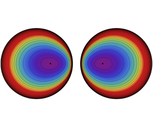
Figure 3. Comparison of (a) the contours of the exact solutions for the fluxes  $J_{1K}$ and $J_{2K}$ with (b) the corresponding contours of the asymptotic solutions for $J_{1}$ and $J_{2}$, and (c) comparisons of $J_{1K}$ and $J_{2K}$ (solid lines) with $J_{1}$ and $J_{2}$ (dashed lines) along the cross-sections $x=\pm 1.1$ ( $-1\leqslant y\leqslant 1$) and $y=0$ ( $-2.1\leqslant x\leqslant -0.1$ and $0.1\leqslant x\leqslant 2.1$) through the centres of the droplets for a pair of identical droplets when $a=1$ and $b=2.2$.
Secondly, for the particular case  $b=2.2$, corresponding to two relatively closely spaced droplets, figure 3 shows a comparison of the contours of the exact solutions for the fluxes $J_{1K}$ and $J_{2K}$ (figure 3a) with the corresponding contours of the asymptotic solutions for $J_{1}$ and $J_{2}$ (figure 3b), and comparisons of $J_{1K}$ and $J_{2K}$ (solid lines) with $J_{1}$ and $J_{2}$ (dashed lines) along the cross-sections $x=\pm 1.1$ ( $-1\leqslant y\leqslant 1$) and $y=0$ ( $-2.1\leqslant x\leqslant -0.1$ and $0.1\leqslant x\leqslant 2.1$) through the centres of the droplets (figure 3c). As figure 3 shows, the asymptotic model accurately captures the shielding effect: evaporation is depressed on the side of the droplet that is closer to the other droplet, resulting in asymmetric profiles of $J_{1}$ and $J_{2}$ along the line $y=0$ (but symmetric profiles along the lines $x=\pm b/2=\pm 1.1$). Again, despite the asymptotic model being formally valid only for well-separated droplets, the agreement with the exact solution in this case of two relatively closely spaced droplets is excellent. In particular, in this case the prediction for the minimum value of the flux is in error by only $1.65\,\%$.
Finally, we note that for further validation we also developed a finite-difference-based code to solve the original governing equations (2.2)–(2.4) numerically. However, despite using  $O(10^{5})$ points we found that convergence to the desired number of decimal places could not be attained, due to the singularities at the contact lines. Indeed, in the present case of two identical droplets we found that the asymptotic model is generally accurate to more decimal places than the solution obtained via our finite-difference-based code.
4 Evolutions and lifetimes of droplets
Encouraged by the excellent agreement between the predictions of the asymptotic model and exact solution for a pair of identical droplets described in § 3.5, we now use the solutions of (3.2) for the integral fluxes  $F_{k}$ for $k=1,\ldots ,N$ to determine the evolutions, and hence the lifetimes, of any configuration of droplets.
Denoting the (small) contact angle of the  $k$th droplet by $\unicode[STIX]{x1D703}_{k}$, its free surface profile by $z=h_{k}$, and its volume by $V_{k}$, we scale $\unicode[STIX]{x1D703}_{k}$, $h_{k}$, $V_{k}$ and time $t$ according to
 $$\begin{eqnarray}\unicode[STIX]{x1D703}_{k}=\unicode[STIX]{x1D703}_{ref}\hat{\unicode[STIX]{x1D703}}_{k},\quad h_{k}=a_{ref}\unicode[STIX]{x1D703}_{ref}{\hat{h}}_{k},\quad V_{k}=a_{ref}^{3}\unicode[STIX]{x1D703}_{ref}\hat{V}_{k},\quad t=\frac{\unicode[STIX]{x1D70C}_{fluid}a_{ref}^{2}\unicode[STIX]{x1D703}_{ref}}{D(c_{sat}-c_{\infty })}\hat{t},\end{eqnarray}$$
 where  $\unicode[STIX]{x1D703}_{ref}$ is a characteristic contact angle, $\unicode[STIX]{x1D70C}_{fluid}$ is the constant density of the fluid and the hats are again immediately dropped. For droplets small enough that surface-tension effects dominate gravitational effects, we have
 $$\begin{eqnarray}h_{k}=\frac{a_{k}\unicode[STIX]{x1D703}_{k}}{2}\left(1-\frac{\unicode[STIX]{x1D70C}^{2}}{a_{k}^{2}}\right),\quad V_{k}=2\unicode[STIX]{x03C0}\int _{0}^{a_{k}}h_{k}\,\unicode[STIX]{x1D70C}\,\text{d}\unicode[STIX]{x1D70C}=\frac{\unicode[STIX]{x03C0}a_{k}^{3}\unicode[STIX]{x1D703}_{k}}{4},\end{eqnarray}$$
 where we now allow both their radii  $a_{k}=a_{k}(t)$ and their contact angles $\unicode[STIX]{x1D703}_{k}=\unicode[STIX]{x1D703}_{k}(t)$, and hence their free surface profiles $h_{k}=h_{k}(\unicode[STIX]{x1D70C},t)$ and their volumes $V_{k}=V_{k}(t)$, to be functions of time. For simplicity, we assume that the distances between the centres of the droplets remain fixed, but other regimes are, in principle, treatable within the same framework. The rate of decrease of the volume of the $k$th droplet is given by the integral flux $F_{k}$, i.e. $-\text{d}V_{k}/\text{d}t=F_{k}$, and hence
 $$\begin{eqnarray}\frac{\text{d}}{\text{d}t}(a_{k}^{3}\unicode[STIX]{x1D703}_{k})=-\frac{4F_{k}}{\unicode[STIX]{x03C0}}.\end{eqnarray}$$
4.1 Evolution and lifetime of a pair of identical droplets
For the pair of identical droplets each with radius  $a=a(t)$, contact angle $\unicode[STIX]{x1D703}=\unicode[STIX]{x1D703}(t)$ and volume $V=V(t)$ a distance $b$ apart analysed in § 3.3, substituting the solution for $F$ given by (3.4) into (4.3) gives
 $$\begin{eqnarray}\frac{\text{d}}{\text{d}t}(a^{3}\unicode[STIX]{x1D703})=-\frac{16a}{\unicode[STIX]{x03C0}[1+(2/\unicode[STIX]{x03C0})\arcsin (a/b)]}.\end{eqnarray}$$
 We consider three modes of evaporation (Picknett & Bexon Reference Picknett and Bexon1977; Stauber et al. Reference Stauber, Wilson, Duffy and Sefiane2014, Reference Stauber, Wilson, Duffy and Sefiane2015), namely the extreme constant radius (CR) mode for which  $a\equiv \bar{a}$ and $\unicode[STIX]{x1D703}=\unicode[STIX]{x1D703}(t)$ subject to the initial condition $\unicode[STIX]{x1D703}(0)=\bar{\unicode[STIX]{x1D703}}$, the extreme constant angle (CA) mode for which $\unicode[STIX]{x1D703}\equiv \bar{\unicode[STIX]{x1D703}}$ and $a=a(t)$ subject to the initial condition $a(0)=\bar{a}$ and the intermediate stick–slide (SS) mode for which $a\equiv \bar{a}$ and $\unicode[STIX]{x1D703}=\unicode[STIX]{x1D703}(t)$ until $\unicode[STIX]{x1D703}$ reaches its critical (receding) value $\unicode[STIX]{x1D703}=\unicode[STIX]{x1D703}^{\star }$ ( $0\leqslant \unicode[STIX]{x1D703}^{\star }\leqslant \bar{\unicode[STIX]{x1D703}}$) at the de-pinning time $t=t^{\star }$, and thereafter $\unicode[STIX]{x1D703}\equiv \unicode[STIX]{x1D703}^{\star }$ and $a=a(t)$ subject to the initial condition $\unicode[STIX]{x1D703}(0)=\bar{\unicode[STIX]{x1D703}}$, where $\bar{a}$ and $\bar{\unicode[STIX]{x1D703}}$ are constants (both of which may, without loss of generality, be set equal to unity, but are retained in what follows for clarity). Note that the SS mode reduces to the CR mode in the limiting case $\unicode[STIX]{x1D703}^{\star }=0$ and to the CA mode in the limiting case $\unicode[STIX]{x1D703}^{\star }=\bar{\unicode[STIX]{x1D703}}$.
(a) Constant radius mode
Setting  $a\equiv \bar{a}$ in (4.4) gives
 $$\begin{eqnarray}\frac{\text{d}\unicode[STIX]{x1D703}}{\text{d}t}=-\frac{16}{\unicode[STIX]{x03C0}\bar{a}^{2}[1+(2/\unicode[STIX]{x03C0})\arcsin (\bar{a}/b)]},\end{eqnarray}$$
 which readily yields the exact solutions for the evolutions of  $\unicode[STIX]{x1D703}$ and $V$, namely
 $$\begin{eqnarray}\unicode[STIX]{x1D703}=\bar{\unicode[STIX]{x1D703}}-\frac{16t}{\unicode[STIX]{x03C0}\bar{a}^{2}\left[1+(2/\unicode[STIX]{x03C0})\arcsin (\bar{a}/b)\right]},\quad V=\frac{\unicode[STIX]{x03C0}\bar{a}^{3}\bar{\unicode[STIX]{x1D703}}}{4}-\frac{4\bar{a}t}{1+(2/\unicode[STIX]{x03C0})\arcsin (\bar{a}/b)}.\end{eqnarray}$$
 In particular, the lifetime of the droplets in the CR mode, denoted by  $t_{CR}$, is determined by setting $V=0$ in (4.6) to obtain
 $$\begin{eqnarray}t_{CR}=\left(1+\frac{2}{\unicode[STIX]{x03C0}}\arcsin \frac{\bar{a}}{b}\right){t_{CR}}_{\infty },\end{eqnarray}$$
 where  ${t_{CR}}_{\infty }=\unicode[STIX]{x03C0}\bar{a}^{2}\bar{\unicode[STIX]{x1D703}}/16$ is the lifetime of the same droplets evaporating in isolation, which is recovered when the distance between the droplets becomes large, i.e. $t_{CR}\rightarrow {t_{CR}}_{\infty }^{+}$ as $b\rightarrow \infty$. Note that in the opposite limit of touching droplets, $b\rightarrow 2\bar{a}^{+}$, then $t_{CR}\rightarrow (4/3)\,{t_{CR}}_{\infty }^{-}$.
(b) Constant angle mode
Setting  $\unicode[STIX]{x1D703}\equiv \bar{\unicode[STIX]{x1D703}}$ in (4.4) gives
 $$\begin{eqnarray}\frac{\text{d}a}{\text{d}t}=-\frac{16}{3\unicode[STIX]{x03C0}a\bar{\unicode[STIX]{x1D703}}[1+(2/\unicode[STIX]{x03C0})\arcsin (a/b)]},\end{eqnarray}$$
 which yields the implicit solutions for the evolution of  $a$ and hence of $V=\unicode[STIX]{x03C0}a^{3}\bar{\unicode[STIX]{x1D703}}/4$, namely
 $$\begin{eqnarray}t=\frac{3\unicode[STIX]{x03C0}\bar{\unicode[STIX]{x1D703}}}{16}[I(\bar{a})-I(a)],\end{eqnarray}$$
 where the function  $I=I(a)$ is defined by
 $$\begin{eqnarray}I=\int _{0}^{a}\hat{a}\left[1+\frac{2}{\unicode[STIX]{x03C0}}\arcsin \frac{\hat{a}}{b}\right]\,\text{d}\hat{a},\end{eqnarray}$$
and hence is given by
 $$\begin{eqnarray}I=\frac{1}{2\unicode[STIX]{x03C0}}\left[\unicode[STIX]{x03C0}a^{2}+a\sqrt{b^{2}-a^{2}}-(b^{2}-2a^{2})\arcsin \frac{a}{b}\right].\end{eqnarray}$$
 In particular, the lifetime of the droplets in the CA mode, denoted by  $t_{CA}$, is given by
 $$\begin{eqnarray}t_{CA}=\frac{3\unicode[STIX]{x03C0}\bar{\unicode[STIX]{x1D703}}I(\bar{a})}{16}=\frac{2I(\bar{a})}{\bar{a}^{2}}{t_{CA}}_{\infty },\end{eqnarray}$$
i.e.
 $$\begin{eqnarray}t_{CA}=\left[1+\frac{1}{\unicode[STIX]{x03C0}\bar{a}^{2}}\left\{\bar{a}\sqrt{b^{2}-\bar{a}^{2}}-\left(b^{2}-2\bar{a}^{2}\right)\arcsin \frac{\bar{a}}{b}\right\}\right]{t_{CA}}_{\infty },\end{eqnarray}$$
 where  ${t_{CA}}_{\infty }=3\unicode[STIX]{x03C0}\bar{a}^{2}\bar{\unicode[STIX]{x1D703}}/32$ is the lifetime of the same droplets evaporating in isolation, i.e. $t_{CA}\rightarrow {t_{CA}}_{\infty }^{+}$ as $b\rightarrow \infty$. Note that in the opposite limit of initially touching droplets, $b\rightarrow 2\bar{a}^{+}$, then $t_{CA}\rightarrow (2\unicode[STIX]{x03C0}+3\sqrt{3})/(3\unicode[STIX]{x03C0})\,{t_{CA}}_{\infty }^{-}\simeq 1.218\,{t_{CA}}_{\infty }^{-}$.
(c) Stick–slide mode
In the SS mode, the droplets initially evaporate in a CR phase satisfying (4.5) according to (4.6) until  $\unicode[STIX]{x1D703}=\unicode[STIX]{x1D703}^{\star }$, which occurs at $t=t^{\star }$, where $t^{\star }$ is given by
 $$\begin{eqnarray}t^{\star }=\frac{\unicode[STIX]{x03C0}\bar{a}^{2}}{16}\left(1+\frac{2}{\unicode[STIX]{x03C0}}\arcsin \frac{\bar{a}}{b}\right)(\bar{\unicode[STIX]{x1D703}}-\unicode[STIX]{x1D703}^{\star }).\end{eqnarray}$$
 Thereafter, the droplets evaporate in a CA phase satisfying (4.8) with  $\bar{\unicode[STIX]{x1D703}}$ replaced by $\unicode[STIX]{x1D703}^{\star }$ according to
 $$\begin{eqnarray}t-t^{\star }=\frac{3\unicode[STIX]{x03C0}\unicode[STIX]{x1D703}^{\star }}{16}[I(\bar{a})-I(a)],\end{eqnarray}$$
 where the function  $I=I(a)$ is again given by (4.11). In particular, the lifetime of the droplets in the SS mode, denoted by $t_{SS}$, is given by
 $$\begin{eqnarray}t_{SS}=t^{\star }+\frac{3\unicode[STIX]{x03C0}\unicode[STIX]{x1D703}^{\star }I(\bar{a})}{16}=\frac{2\left[\bar{a}^{2}(1+(2/\unicode[STIX]{x03C0})\arcsin (\bar{a}/b))(\bar{\unicode[STIX]{x1D703}}-\unicode[STIX]{x1D703}^{\star })+3\unicode[STIX]{x1D703}^{\star }I(\bar{a})\right]}{\bar{a}^{2}(2\bar{\unicode[STIX]{x1D703}}+\unicode[STIX]{x1D703}^{\star })}{t_{SS}}_{\infty },\end{eqnarray}$$
i.e.
 $$\begin{eqnarray}t_{SS}=\left[1+\frac{(2\bar{a}^{2}(2\bar{\unicode[STIX]{x1D703}}+\unicode[STIX]{x1D703}^{\star })-3b^{2}\unicode[STIX]{x1D703}^{\star })\arcsin (\bar{a}/b)+3\bar{a}\unicode[STIX]{x1D703}^{\star }\sqrt{b^{2}-\bar{a}^{2}}}{\unicode[STIX]{x03C0}\bar{a}^{2}(2\bar{\unicode[STIX]{x1D703}}+\unicode[STIX]{x1D703}^{\star })}\right]{t_{SS}}_{\infty },\end{eqnarray}$$
 where  ${t_{SS}}_{\infty }=\unicode[STIX]{x03C0}\bar{a}^{2}(2\bar{\unicode[STIX]{x1D703}}+\unicode[STIX]{x1D703}^{\ast })/32$ is the lifetime of the same droplets evaporating in isolation, i.e. $t_{SS}\rightarrow {t_{SS}}_{\infty }^{+}$ as $b\rightarrow \infty$. Note that in the opposite limit of initially touching droplets, $b\rightarrow 2\bar{a}^{+}$, then
 $$\begin{eqnarray}t_{SS}\rightarrow \frac{8\unicode[STIX]{x03C0}\bar{\unicode[STIX]{x1D703}}+(9\sqrt{3}-2\unicode[STIX]{x03C0})\unicode[STIX]{x1D703}^{\star }}{3\unicode[STIX]{x03C0}(2\bar{\unicode[STIX]{x1D703}}+\unicode[STIX]{x1D703}^{\star })}{t_{SS}}_{\infty }^{-}.\end{eqnarray}$$
Figure 4. The lifetimes of (a) a pair of identical droplets and (b) a polygonal array of  $N=5$ identical droplets evaporating in the CR ( $\unicode[STIX]{x1D703}^{\star }=0$), CA ( $\unicode[STIX]{x1D703}^{\star }=1$) and SS ( $\unicode[STIX]{x1D703}^{\star }=1/5$, $2/5,3/5$ and $4/5$) modes of evaporation plotted as functions of $b$ when $\bar{a}=1$ and $\bar{\unicode[STIX]{x1D703}}=1$. The dots denote the limiting values in the limit $b\rightarrow 2^{+}$ in (a) and in the limit $b\rightarrow 2/\sin (\unicode[STIX]{x03C0}/5)^{+}\simeq 3.403^{+}$ in (b), and the horizontal dashed lines denote the limiting values in the limit $b\rightarrow \infty$.
Figure 4(a) shows  $t_{CR}$, $t_{CA}$ and $t_{SS}$ given by (4.7), (4.13) and (4.17), respectively, plotted as functions of $b\,({\geqslant}2)$ when $\bar{a}=1$ and $\bar{\unicode[STIX]{x1D703}}=1$. In particular, figure 4(a) shows that, due to the shielding effect, $t_{CR}$, $t_{CA}$ and $t_{SS}$ are all monotonically decreasing functions of $b$ for fixed $\unicode[STIX]{x1D703}^{\star }$ (i.e. the lifetime of a pair of droplets is always longer than that of the same droplets in isolation), but monotonically increasing functions of $\unicode[STIX]{x1D703}^{\star }$ for fixed $b$ (i.e. the lifetime of the droplets in the SS mode always lies between that of the same droplets in the extreme modes, $t_{CR}\leqslant t_{SS}\leqslant t_{CA}$). Furthermore, as figure 4(a) also shows, while the relative impact of the shielding effect on the lifetime of the droplets decreases slightly with $\unicode[STIX]{x1D703}^{\star }$, even touching droplets evaporating in the CR mode (i.e. $t_{CR}\rightarrow \unicode[STIX]{x03C0}\bar{a}^{2}\bar{\unicode[STIX]{x1D703}}/12^{-}$ in the limit $b\rightarrow 2\bar{a}^{+}$) still have a shorter lifetime than isolated droplets evaporating in the CA mode (i.e. $t_{CA}\rightarrow 3\unicode[STIX]{x03C0}\bar{a}^{2}\bar{\unicode[STIX]{x1D703}}/32^{+}$ in the limit $b\rightarrow \infty$).
4.2 Evolution and lifetime of a polygonal array of $N$ identical droplets

Following the same approach as in § 4.1, we can obtain the corresponding expressions for the evolution and lifetimes of the polygonal array of  $N$ identical droplets analysed in § 3.4 governed by
 $$\begin{eqnarray}\frac{\text{d}}{\text{d}t}(a^{3}\unicode[STIX]{x1D703})=-\frac{16a}{\unicode[STIX]{x03C0}\left[1+(2/\unicode[STIX]{x03C0})\mathop{\sum }_{n=1}^{N-1}\arcsin (a/b_{n})\right]},\end{eqnarray}$$
 simply by replacing  $\arcsin (a/b)$ with $\sum _{n=1}^{N-1}\arcsin (a/b_{n})$, where $b_{n}$ is given by (3.8), and the function $I(a)$ with $I_{N}(a)$ defined by
 $$\begin{eqnarray}I_{N}=\int _{0}^{a}\hat{a}\left[1+\frac{2}{\unicode[STIX]{x03C0}}\mathop{\sum }_{n=1}^{N-1}\arcsin \frac{\hat{a}}{b_{n}}\right]\,\text{d}\hat{a},\end{eqnarray}$$
and hence given by
 $$\begin{eqnarray}I_{N}=\frac{1}{2\unicode[STIX]{x03C0}}\left[\unicode[STIX]{x03C0}a^{2}+\mathop{\sum }_{n=1}^{N-1}\left\{a\sqrt{b_{n}^{2}-a^{2}}-(b_{n}^{2}-2a^{2})\arcsin \frac{a}{b_{n}}\right\}\right],\end{eqnarray}$$
in the appropriate places. In particular, the lifetime of the droplets in the SS mode (from which the lifetime of the droplets in the extreme modes can readily be deduced) is given by
 $$\begin{eqnarray}t_{SS}\,=\,\left[\!1+\frac{1}{\unicode[STIX]{x03C0}\bar{a}^{2}(2\bar{\unicode[STIX]{x1D703}}+\unicode[STIX]{x1D703}^{\star })}\mathop{\sum }_{n=1}^{N-1}\left\{\!(2\bar{a}^{2}(2\bar{\unicode[STIX]{x1D703}}+\unicode[STIX]{x1D703}^{\star })-3\unicode[STIX]{x1D703}^{\star }b_{n}^{2})\arcsin \frac{\bar{a}}{b_{n}}+3\bar{a}\unicode[STIX]{x1D703}^{\star }\sqrt{b_{n}^{2}-\bar{a}^{2}}\right\}\!\right]{t_{SS}}_{\infty }.\end{eqnarray}$$
 Figure 4(b) shows  $t_{CR}$, $t_{CA}$ and $t_{SS}$ for a polygonal array of $N=5$ droplets plotted as functions of $b\,({\geqslant}2/\sin (\unicode[STIX]{x03C0}/5)\simeq 3.403)$ when $\bar{a}=1$ and $\bar{\unicode[STIX]{x1D703}}=1$. In particular, figure 4(b), which is typical of the corresponding results for all values of $N\geqslant 3$, shows that the behaviour of a polygonal array of $N$ identical droplets is qualitatively similar to that of a pair of identical droplets (i.e. to that in the special case $N=2$ shown in figure 4a). However, as figure 4(b) illustrates, touching droplets evaporating in the CR mode having a shorter lifetime than isolated droplets evaporating in the CA mode is peculiar to the special case $N=2$.
5 Radially integrated evaporative flux $R_{k}$

We now examine how the radially integrated evaporative flux from the  $k$th droplet, denoted by $R_{k}=R_{k}(\unicode[STIX]{x1D719})$ and given by
 $$\begin{eqnarray}R_{k}=\int _{0}^{a_{k}}J_{k}(\unicode[STIX]{x1D70C},\unicode[STIX]{x1D719})\,\unicode[STIX]{x1D70C}\,\text{d}\unicode[STIX]{x1D70C},\end{eqnarray}$$
 varies with the local polar angle  $\unicode[STIX]{x1D719}$. As discussed below, this quantity is of particular interest because of its connection to the coffee-ring effect.
For the pair of identical droplets analysed in § 3.3, substituting the solution for  $J_{1}$ given by (3.5) into (5.1) gives the radially integrated flux in the droplet centred at $(-b/2,0)$, denoted by $R_{1}(\unicode[STIX]{x1D719})$, to be
 $$\begin{eqnarray}R_{1}=R_{0}\left[1-\frac{F\sqrt{1-k^{2}}}{2\unicode[STIX]{x03C0}a\sin \unicode[STIX]{x1D719}}\text{Im}\left\{\frac{\log \left[-\left(k\text{e}^{-\text{i}\unicode[STIX]{x1D719}}+\sqrt{k^{2}\text{e}^{-2\text{i}\unicode[STIX]{x1D719}}-1}\right)\right]}{\sqrt{k^{2}\text{e}^{-2\text{i}\unicode[STIX]{x1D719}}-1}}\right\}\right],\end{eqnarray}$$
 where  $k=a/b$, $R_{0}=2a/\unicode[STIX]{x03C0}$ is the radially integrated flux from an isolated droplet, and $F$ is given by (3.4). The corresponding expression for the radially integrated flux in the other droplet centred at $(b/2,0)$, denoted by $R_{2}(\unicode[STIX]{x1D719})$, is obtained by replacing $\unicode[STIX]{x1D719}$ with $\unicode[STIX]{x1D719}+\unicode[STIX]{x03C0}$ in (5.2). In particular, in the limit $k=a/b\rightarrow 0$ we have
 $$\begin{eqnarray}R_{1}=R_{0}\left[1-\frac{2}{\unicode[STIX]{x03C0}}\frac{a}{b}+\left(\frac{4}{\unicode[STIX]{x03C0}^{2}}-\cos \unicode[STIX]{x1D719}\right)\left(\frac{a}{b}\right)^{2}+O\left(\frac{a}{b}\right)^{3}\right].\end{eqnarray}$$
Figure 5. Comparison between the exact solution (solid lines), the asymptotic solution given by (5.2) (dashed lines) and the expansion of the asymptotic solution given by (5.3) (dotted lines, indistinguishable from the solid line for  $b=10$) for the radially integrated evaporative flux $R_{1}$ from the droplet centred at $(-b/2,0)$ for the pair of identical droplets analysed in § 3.3 plotted as functions of the scaled local polar angle $\unicode[STIX]{x1D719}/\unicode[STIX]{x03C0}$ when $a=1$ for $b=2$, 6 and 10. The direction of the arrow corresponds to increasing values of $b$. The horizontal line $R_{1}=R_{0}=2a/\unicode[STIX]{x03C0}\simeq 0.637$ corresponds to the limiting value of $R_{1}$ in the limit $b\rightarrow \infty$.
In order to assess the accuracy of the expressions (5.2) and (5.3), figure 5 shows a comparison of them with the exact solution for the radially integrated flux  $R_{1}$ computed using the formulation due to Kobayashi (Reference Kobayashi1939) as described in § 3.5 for three different values of $b$. In particular, figure 5 shows that the asymptotic solution (5.2) is quite accurate even for relatively large values of $a/b$, but, as expected, the expansion of the asymptotic solution (5.3) is a useful approximation only for sufficiently small values of $a/b$.
Sáenz et al. (Reference Sáenz, Wray, Che, Matar, Valluri, Kim and Sefiane2017) demonstrated that, for a droplet containing nanoparticles evaporating in the CR mode, the distribution of the final residue is strongly related to the radially integrated fluid flux within the droplet, which is in turn closely related to the radially integrated evaporative flux  $R_{k}$. In particular, the radial directions with the greatest values of $R_{k}$ have the greatest fluid flux within the droplet, giving the greatest concentration of residue at the contact line in that direction. Of course, because of other effects, such as particle diffusion and azimuthal flow, $R_{k}$ does not give a perfect characterisation of the final residue distribution. However, Sáenz et al. (Reference Sáenz, Wray, Che, Matar, Valluri, Kim and Sefiane2017) observed that even in the highly asymmetric case of a triangular droplet the flow is predominantly radial, and in many situations $R_{k}$ will indeed provide a good indication of what final residue will occur. The solutions for $R_{1}$ for a pair of identical droplets shown in figure 5 reveal that, as expected, the azimuthal variation of $R_{1}$ is most pronounced when the droplets are closest together (i.e. when the shielding effect is most significant), and so we would anticipate that this situation would give rise to the most non-homogeneous coffee rings, with least residue accumulating where the contact lines are closest together and most residue accumulating where they are furthest apart.
6 Comparison with the experimental results of Khilifi et al. (Reference Khilifi, Foudhil, Fahem, Harmand and Ben Jabrallah2019)
The ultimate test for the value of the present asymptotic model is, of course, how well its theoretical predictions compare with experimental results. To this end, we compare the theoretical predictions of the present model with the recent experimental results of Khilifi et al. (Reference Khilifi, Foudhil, Fahem, Harmand and Ben Jabrallah2019) for seven relatively closely spaced droplets.
Khilifi et al. (Reference Khilifi, Foudhil, Fahem, Harmand and Ben Jabrallah2019) studied the evaporation of sessile droplets of water at an initial temperature of  $20\,^{\circ }\text{C}$ on a sapphire substrate into an enclosed chamber with 50 % humidity at an ambient temperature of $21\,^{\circ }\text{C}$. Initial experiments using an isolated droplet revealed that the droplets evaporate in an SS mode with an initial contact angle of $\bar{\unicode[STIX]{x1D703}}\simeq 80^{\circ }$ and a receding contact angle of $\unicode[STIX]{x1D703}^{\star }\simeq 36^{\circ }$. To investigate the interactions between the droplets, they then studied a (slightly imperfect) ‘I’-shaped configuration of seven nearly identical droplets with approximate radius $7.5\times 10^{-4}~\text{m}$ and volume $7\times 10^{-10}~\text{m}^{3}$ a distance $2\times 10^{-4}~\text{m}$ apart (their ‘Configuration (b)’).

Figure 6. Comparison between the theoretical predictions of the present model (dashed lines) and the corresponding experimental results of Khilifi et al. (Reference Khilifi, Foudhil, Fahem, Harmand and Ben Jabrallah2019) (solid lines) for the planform of seven droplets in an ‘I’-shaped configuration at six different dimensional times (in seconds). The initial planforms are shown with grey lines.
Figure 6 shows the comparison between the theoretical predictions of the present model (dashed lines) and the corresponding experimental results of Khilifi et al. (Reference Khilifi, Foudhil, Fahem, Harmand and Ben Jabrallah2019) (solid lines) for the planform of the droplets at six different dimensional times. The theoretical results were calculated by solving the seven evolution equations (4.3) for  $k=1,2,\ldots ,7$ with the $F_{k}$ obtained from (3.2) numerically using a fourth-order Runge–Kutta method using the parameter values $\unicode[STIX]{x1D70C}=997.79~\text{kg}~\text{m}^{-3}$, $D=2.43\times 10^{-5}~\text{m}^{2}~\text{s}^{-1}$ and $c_{sat}=1.83\times 10^{-2}~\text{kg}~\text{m}^{-3}$, the former value being calculated from Raznjevic (Reference Raznjevic1995, table 33-11) and the latter two values being calculated from Monteith & Unsworth (Reference Monteith and Unsworth2013, tables A.3 and A.4) using a temperature of $21\,^{\circ }\text{C}$. The experimental results of Khilifi et al. (Reference Khilifi, Foudhil, Fahem, Harmand and Ben Jabrallah2019) were extracted from their figure 6(b) using an edge-detection algorithm. As both the theoretical and experimental results show, the four droplets at the corners of the ‘I’ experience the weakest shielding effect and so evaporate the fastest, while the central droplet experiences the strongest shielding effect and so evaporates the slowest. The only significant discrepancy apparent in figure 6 is at dimensional time $t=1700~\text{s}$, at which time the two droplets at the top and the bottom of the ‘I’ have completely evaporated in the experiment but have not yet completely evaporated according to the model. However, at this late stage in their evolution the radii of these droplets are shrinking rapidly, and so the disagreement is a relatively minor one (in fact, the model predicts that complete evaporation of these droplets occurs at dimensional times $t=1724~\text{s}$ and $t=1755~\text{s}$, respectively, with complete evaporation of the central droplet occurring at a dimensional time of $t=1869~\text{s}$.

Figure 7. Comparison between the theoretical predictions (dashed lines) of the present model and the corresponding experimental results of Khilifi et al. (Reference Khilifi, Foudhil, Fahem, Harmand and Ben Jabrallah2019) (solid lines) for the average evolutions of (a) the dimensional diameters  $d=2a$ (in mm) and (b) the contact angles $\unicode[STIX]{x1D703}$ of the three different families of droplets (namely, in increasing order of their lifetimes, the four droplets at the corners of the ‘I’, the two droplets at the top and the bottom of the ‘I’ and the central droplet) plotted as functions of dimensional time $t$ (in seconds).
A further comparison is given in figure 7, which shows the average evolutions of the dimensional diameters  $d=2a$ (figure 7a) and the contact angles $\unicode[STIX]{x1D703}$ (figure 7b) of the three different families of droplets (namely, in increasing order of their lifetimes, the four droplets at the corners of the ‘I’, the two droplets at the top and the bottom of the ‘I’ and the central droplet) plotted as functions of dimensional time $t$.
$t$.
Given the approximations involved in the mathematical model, the inevitable experimental errors and uncertainties in the exact values of the parameters, as well as the relatively large value of the initial contact angle, the agreement between theory and experiment shown in figures 6 and 7 is surprisingly good, and suggests that the present asymptotic model could be a useful tool for studying a wide range of other droplet configurations.
7 Conclusions
In the present work we put the approximate approach of Fabrikant (Reference Fabrikant1985) on an asymptotic basis, before extending the procedure to obtain explicit expressions for the local fluxes from multiple evaporating sessile droplets. The power of the present asymptotic model was then illustrated by obtaining explicit solutions for a pair of and for a polygonal array of identical droplets. In order to verify the accuracy of the model, comparisons were made with the exact solution of the problem for a pair of identical droplets; in particular, the model was found to perform well even outside its formal range of validity, up to and including the limit of touching droplets. The model was used to investigate the shielding effect on droplet evolutions and lifetimes in both configurations, as well as on the coffee-ring effect for a pair of droplets. The theoretical predictions of the model were found to be in good agreement with the recent experimental results of Khilifi et al. (Reference Khilifi, Foudhil, Fahem, Harmand and Ben Jabrallah2019), suggesting that the model could be a useful tool for studying a wide range of other droplet configurations.
Acknowledgements
The authors are grateful to Dr D. Pritchard and Mr F. G. H. Schofield (University of Strathclyde) and Professor K. Sefiane (University of Edinburgh) for insightful discussions about various aspects of droplet evaporation, and, in particular, to Professor Sefiane for encouraging them to investigate the evaporation of multiple droplets. The authors also wish to thank the three anonymous referees of the original version of this work, whose comments and suggestions significantly improved the final version. The authors received no specific funding for this work, and have no conflict of interest with regard to it.


 Open access