


1. Introduction
Steady separation, in two dimensions and from a stationary surface, was classified by Prandtl (Reference Prandtl1904) to occur when the skin friction approaches zero, whilst the separation point remains fixed. This definition, however, is no longer applicable for unsteady separation, where a movement of the separation point may occur, together with a significant time-varying force history which exceeds the steady-state equivalent (Farren Reference Farren1935; Bennett Reference Bennett1970; Sane & Dickinson Reference Sane and Dickinson2001). In an attempt to improve the classification of the unsteady separation point, Moore (Reference Moore1958), Rott (Reference Rott1956) and Sears & Telionis (Reference Sears and Telionis1975) proposed the requirement that the shear stress vanishes within the flow, whilst simultaneously the tangential velocity matches the speed of the separating structure, of which varying success is reported (Ludwig Reference Ludwig1964; Labraga et al. Reference Labraga, Kahissim, Keirsbulck and Beaubert2007).
Unsteady separation occurs during rapidly changing body motion as well as on wings immersed in gusty and turbulent environments (Eldredge & Jones Reference Eldredge and Jones2019), which is a commonly occurring feature of the unsteady atmospheric boundary layer (Watkins et al. Reference Watkins, Milbank, Loxton and Melbourne2006, Reference Watkins, Thompson, Loxton and Abdulrahim2010). Efforts have therefore been undertaken to categorize the unsteady effects, such as the build up of bound circulation on wings (Pitt Ford & Babinsky Reference Pitt Ford and Babinsky2013) or the unsteady shedding of vortices from the leading and trailing edge (Eldredge & Jones Reference Eldredge and Jones2019).
The significant force spike associated with these transient phenomena is of considerable practical interest when computing the unsteady loading in an attempt to inform its mitigation. Micro aerial vehicles (MAV) can suffer from the detrimental effects of highly gusty and turbulent conditions, where even urban canyons can create such chaotic environments (White et al. Reference White, Lim, Watkins, Mohamed and Thompson2012), causing delivery drones or future passenger aircraft to combat unpredictable aerodynamic scenarios. Furthermore, flapping wing MAVs such as the NanoHummmingbird (Keennon, Klingebiel & Won Reference Keennon, Klingebiel and Won2012) or rotary drones or helicopters need to mitigate externally arising turbulent conditions or those created through their own kinematic motions (Hodara et al. Reference Hodara, Lind, Jones and Smith2016). Similar problems are experienced by water turbines (Sequeira & Miller Reference Sequeira and Miller2014), where varying loads caused by waves, tides and gusts can lead to fatigue and failure.
Lengthy numerical computations are not an option to inform real time gust mitigation due to their substantial time requirements, instead, rapid real-time, yet accurate, simulations are essential. Low order models (LOMs), which distil the flow physics into simpler, more tractable problems, appear as promising candidates for such endeavours. However, substantial difficulties arise when the unsteady shedding process is to be integrated into the simulations. Modelling the development of shed vorticity is unfortunately a prerequisite, yet difficult for LOMs, as they only have access to basic flow properties.
One boundary layer property, however, that is easily obtainable, even for LOMs, is the boundary layer vorticity. It develops as the flow field evolves and feeds any vortices that are shed (Xia & Mohseni Reference Xia and Mohseni2017). In simple analytical or numerical models of a flow, the boundary layer is often represented by an infinitely thin vortex sheet located on the body surface. Its strength is related to the vorticity contained in the physical boundary layer and thereby equivalent to an infinitely thin distribution of this vorticity. The vortex sheet arises from the necessity to enforce the non-penetration condition using potential theory, which in turn leads to a slip velocity that can be interpreted as an infinitely thin boundary layer (Saffman Reference Saffman1992). Importantly, this property can be inferred from experimental data (Corkery, Babinsky & Graham Reference Corkery, Babinsky and Graham2019) or calculated through potential flow theory and panel method codes in simulations (Gehlert & Babinsky Reference Gehlert and Babinsky2021). The vortex sheet is in turn the source of shed vorticity that regularly develops in unsteady flow fields, with early attempts of modelling such flows around a cylinder using a vortex sheet- and point vortex-like approach described by Chorin (Reference Chorin1973). Ramesh et al. (Reference Ramesh, Gopalarathnam, Granlund, Ol and Edwards2014) introduced the leading edge suction parameter (LESP) to predict unsteady separation. They propose that whenever the LESP exceeds a predetermined critical value at the leading edge, unsteady separation is initiated. Even though the LESP is often calculated directly from the leading edge pressure, it is intrinsically linked to the boundary layer vorticity and can be calculated from this (Eldredge Reference Eldredge2019). Ramesh (Reference Ramesh2020) further shows that the LESP can be related to the leading edge velocity by expanding the singularity using asymptotic matching of an outer solution, based on thin linear airfoil theory, and an inner solution, formed by evaluating flow past a parabola. Whilst the LESP has been shown to be successful at predicting flow detachment, trailing edge separation (Ramesh et al. Reference Ramesh, Granlund, Ol, Gopalarathnam and Edwards2018) and increased airfoil pitch rates (Deparday & Mulleners Reference Deparday and Mulleners2019) can modify the critical value at which unsteady separation occurs. Furthermore, changing LESP strength has been documented by Deparday & Mulleners (Reference Deparday and Mulleners2019) during vortex shedding as well as by He & Williams (Reference He and Williams2020), the latter investigating the progression of the LESP during attached and separated turbulent surging flow states past an airfoil, further suggesting a variability in the critical LESP strength.
Investigating a pitching wing, Melius, Mulleners & Cal (Reference Melius, Mulleners and Cal2018) note a repeating peak boundary layer vorticity strength at the unsteady separation point. Moreover, a constant strength of shed vorticity is observed for a wing undergoing variable kinematic motions by Deparday & Mulleners (Reference Deparday and Mulleners2019). These observations suggest that there may be a link between the local boundary layer vortex sheet strength and the unsteady separation location.
The aim of this paper is therefore to explore the unsteady development of the boundary layer vorticity in a transient flow with separation. The main focus is to understand what affects the strength of the boundary layer vorticity, and whether any patterns can be observed at the unsteady separation point. This provides an understanding of the fundamental building blocks contributing to the boundary layer vorticity and informs any methods that rely on boundary layer vorticity to predict unsteady separation. To this end, we restrict ourselves to two-dimensional flow for simplicity and focus on the boundary layer development on a circular cylinder. By subjecting the cylinder to translation as well as rotation, it is possible to model lifting bodies and multiple dynamically changing flow fields using a single geometry.
2. Measuring the unsteady cylinder boundary layer development
To investigate the development of the cylinder boundary layer, experiments are performed in the University of Cambridge Towing Tank facility. A circular cylinder with a diameter,  $D$, of 0.06 m is accelerated, or alternatively, a surging and rotation motion is applied to a smaller cylinder, $D = 0.04\ \textrm {mm}$, whilst planar particle image velocimetry (PIV) data are collected to assess the flow field.
2.1. Cylinder kinematics
Three different kinematic cases are explored:
Case 1: the larger circular cylinder,  $D = 0.06\ \textrm {m}$, accelerates linearly from a stationary start until it has travelled a distance, $s$, of three diameters, $s/D =3$. Thereafter, it continues at a constant velocity of $0.43\ \textrm {m}\,\textrm {s}^{-1}$, leading to a Reynolds number, $Re$, of 20 000.
Case 2a: the smaller cylinder,  $D = 0.04\ \textrm {m}$, simultaneously begins to translate and rotate from a stationary start. It accelerates for two diameters after which it continues to translate at a constant velocity of $0.32\ \textrm {m}\,\textrm {s}^{-1}$, giving a Reynolds number of 10 000. It rotates at 153 revolutions per minute, which results in a rotation ratio, $\alpha = ({\varOmega _\infty a})/{U}$ of 0.5. U represents the instantaneous velocity, $\varOmega _\infty$ is the final angular velocity and $a$ is the cylinder radius. A constant angular velocity is reached within $s/D = 0.25$.
Case 2b: the smaller cylinder again follows the same translation and rotation profile as outlined for Case 2a but with  $\alpha$ increased to 2.5. $\varOmega _\infty$ is reached within $s/D = 0.23$.
2.2. Towing tank and cylinder
The towing tank used throughout this investigation is 9 m long, 1 m wide and is filled with water up to 0.8 m. The walls and the floor are made out of glass and a carriage moves the length of the tank, to which the cylinder is vertically mounted, as shown in figure 1(a).

Figure 1. (a) Schematic illustration of the experimental set-up. (b) Sketch of the cylinder assembly.
The cylinder is made from a hollow carbon fibre tube that sits on two bearings. These are attached to a hollow, load bearing, aluminium tube which is clamped to the carriage. A drive shaft is housed inside the tube and connects to the EC synchronous motor via a rotary coupling. The drive shaft further attaches to a 3D printed plug at the far end of the cylinder, which in turn is connected to the carbon fibre cylinder and transmits the rotary motion. The cylinder span is 0.48 m and a skim plate at the top acts as a mirror plane. The effective aspect ratio of the cylinders is therefore extended to 16 and 24 respectively. A schematic illustration of the cylinder design is shown in figure 1(b).
The servo motor driven carriage moves along the length of the tank, in the  $x$-direction, and its position is measured using an electro-optical sensor with a resolution of 1 mm. The velocity is determined through numerical differentiation of the position data and the acceleration is measured using a 3-component micro-electromechanical accelerometer, ADXL335, mounted to the carriage. The rotation speed of the cylinder is acquired using an encoder located on the motor. The cylinder surface velocity can therefore be recorded at each instance and all measurements are sampled at 3000 Hz.
2.3. Particle image velocimetry
Two components of flow velocity are measured using planar PIV in a horizontal plane located at the midspan of the cylinder. A Nd:YLF 527 nm laser is used to illuminate titanium dioxide particles dispersed in the water. The laser optics are offset in the  $x$-direction as to produce two opposing light sheets which are shone into the test section to eliminate any shadow regions as shown in figure 2(a). Two high-speed Phantom M310 cameras are positioned in a dual camera arrangement below the water tank to enable optical access to all regions of the flow field. The sampling frequency is adjusted between 800 and 1100 Hz and 6 repeats are conducted per kinematic test case from which an ensemble average is obtained. The commercial LaVision Flowmaster 2D system is used for the cross-correlation process which is applied to both camera images independently. Thereafter, the two resulting vector fields are stitched together to yield a complete representation of the flow field without any shadow regions. The adaptive interrogation window has a size of $16 \times 16$ pixels during its final pass with an overlap of 50 %, leading to an approximate vector spacing of 1.4 mm.
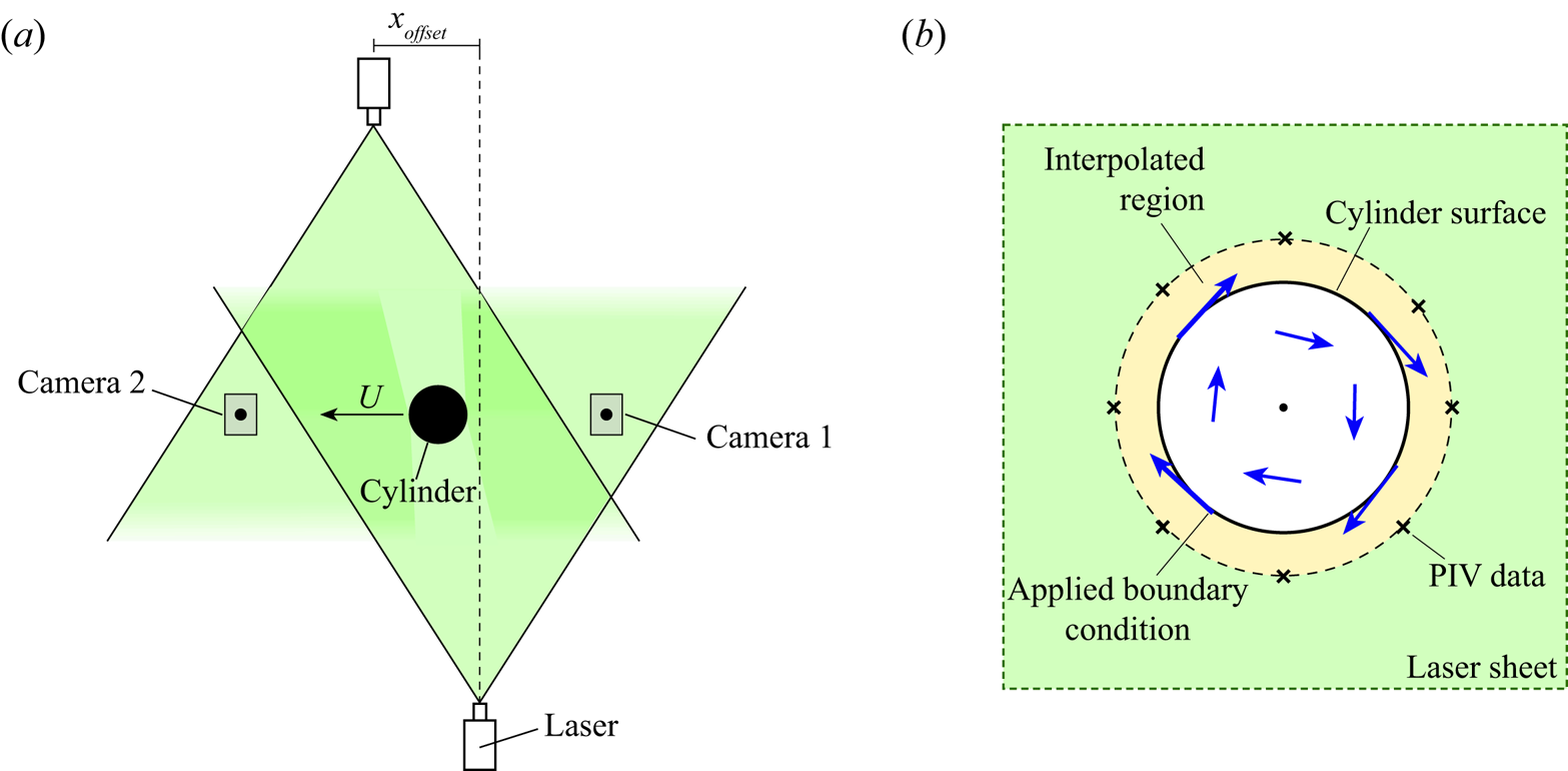
Figure 2. (a) Top view of the experimental set-up. (b) Schematic illustration of the interpolation process used to recover missing velocity vectors directly around the cylinder.
Laser reflections from the matte black painted cylinder cause some missing velocity data close to the cylinder surface. However, by interpolating between the measured velocity field and the known cylinder surface velocity, obtained by tracking the cylinder kinematics, boundary layer vorticity data can be recovered as schematically illustrated in figure 2(b) and discussed in § 2.4. This study focuses on assessing the boundary layer vorticity magnitude, rather than on details of the vorticity distribution within the boundary layer. Therefore problems due to reflections extending approximately 0.02  $D$ into the flow field do not adversely influence the results.
The image of the titanium particles seen by the cameras is adjusted so that the particle diameter is smeared over more than 2 pixels. This ensures that peak-locking effects do not dominate the root square velocity error estimation (Westerweel Reference Westerweel1997). The particle displacement in the experiments is between 3 and 4 pixels, which leads to a conservative error estimate of 0.6 %, according to Raffel et al. (Reference Raffel, Willert, Wereley and Kompenhans1998). To further categorize the error in the PIV measurements, the shift in the correlation peak when mapping an interrogation window back to its original position according to the calculated displacement vector (Wieneke Reference Wieneke2015) is used. An uncertainty of 6 % relative to  $U_\infty$ is subsequently calculated in regions of interest for an individual run. In order to reduce the associated error, each kinematic case is repeated six times and the post-processed flow field is averaged. The error consequently reduces to 3 % as the uncertainty scales with $1/\sqrt {N}$, where $N$ is the number of repeated runs (Adrian & Westerweel Reference Adrian and Westerweel2011). The total uncertainty of the velocity measurements obtained through PIV is therefore below 4 %.
2.4. Measuring the boundary layer vorticity
The aim of the experiments is to determine the strength of the boundary layer vortex sheet which derives from the boundary layer vorticity. Despite the fact that the boundary layer velocity distribution is not fully resolved, it is possible to determine the boundary vorticity magnitude as long as the tangential boundary layer edge velocity as well as cylinder surface motion is known.
To robustly compute the vortex sheet strength experimentally, the cylinder surface and the surrounding flow field are split up into  $n$ wedges, as schematically illustrated in figure 3. The circulation contained within each wedge is now computed by integrating the velocity, $u$, aligned with the contour of each wedge ${\rm d}l$,
 \begin{equation} \delta \varGamma_n = \oint u \, \textrm{d}l. \end{equation}
The velocity along the cylinder is set to the true surface velocity, and linear interpolation is used to obtain the flow velocity along the integration path, as it cannot be guaranteed that PIV velocity vectors lie exactly on the specified contour of each wedge. The vortex sheet strength is ultimately obtained by dividing  $\delta \varGamma _n$ by the segment length $\delta s_n$,
 \begin{equation} \gamma_n = \frac{\delta \varGamma_n}{\delta s_n}. \end{equation}
In the current paper 70 elements are used to compute the boundary layer vortex sheet. Increasing the number of elements further results in the same distribution albeit with slightly more noise.

Figure 3. Discretization of the cylinder and surrounding flow field to obtain  $\gamma ^b$ from experimental data.
3. Evolution of the cylinder boundary layer
3.1. Surge only
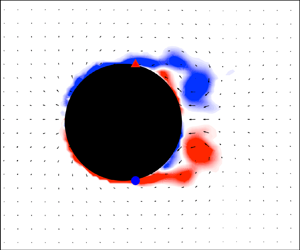
The first flow field to be explored is that created by a translating cylinder, Case 1, as shown by several ‘vorticity’ snapshots in figure 4. The cylinder begins to translate from right to left and linearly accelerates until  $s/D = 3$ after which it moves at a constant speed.

Figure 4. Normalized vorticity contours as the cylinder translates, Case 1; (a)  $s/D = 0.3$, (b) $s/D = 0.7$, (c) $s/D = 1.5$, (d) $s/D = 2.0$, (e) $s/D = 3.0$, ( f) $s/D = 4.5$.
Throughout the time period under investigation, the flow is more or less symmetrical about the  $x$-axis running through the cylinder centre and initially remains attached. An inspection of the time-resolved PIV data suggests that separation becomes clearly visible at approximately $s/D = 0.9$. The unsteady separation points are located on the downstream side of the cylinder, where they slowly move upstream along the cylinder surface as the flow develops and more vorticity is shed. The separating shear layers roll up into two vortices which remain close to the surface throughout the captured motion, whilst at the same time growing in size as the translation distance increases.
Before separation is observed,  $s/D < 0.9$, the experimental flow field closely resembles potential flow around a circular cylinder. This is demonstrated in figure 5(a) where the streamlines, recovered from the PIV measurements, are reminiscent of those calculated using potential theory.

Figure 5. (a) Vorticity contours and streamlines reminiscent of those observed in potential cylinder flow, when the cylinder has just started moving. (b) Theoretical and measured boundary layer vortex sheet at selected time intervals.
The boundary layer vortex sheet,  $\gamma ^b$, determined at these early instances is plotted in figure 5(b) together with its theoretical equivalent. Whilst the experimental vortex sheet is obtained using the methodology outlined in § 2.4, the theoretical distribution, $\gamma ^{tr}$, is computed from the slip velocity between the cylinder surface and the surrounding potential flow. Using this approach, the theoretical vortex sheet distribution is equal to
 \begin{equation} \gamma^{tr} ={-}2U\sin \theta, \end{equation}
where  $U$ is the instantaneous velocity and $\theta$ is the surface definition as indicated in figure 5(a). As the cylinder accelerates, the amplitude of the sinusoidal distributions of both the experimental and theoretical vortex sheets grow, and a close match between the two is observed. This therefore suggests, that before any vorticity is shed, the boundary layer vortex sheet, and hence the boundary layer vorticity, is only a function of the cylinder geometry and the kinematic motion.
As the cylinder continues to accelerate, the flow separates and vorticity sheds from its surface, as seen in figure 4(c–f). This has a significant effect on the boundary layer vortex sheet, as shown in figure 6. The development of the vortex sheet is similar to that computed by Bar-lev & Yang (Reference Bar-lev and Yang1975), who modelled the flow about an impulsively started cylinder using a matched asymptotic expansion and arrived at a comparable distribution of boundary layer vorticity. Further similarities appear when observing the boundary layer vorticity distribution provided by Koumoutsakos & Leonard (Reference Koumoutsakos and Leonard1995), where the flow is modelled using a viscous vortex model.

Figure 6. Evolution of  $\gamma ^b$, Case 1. Line colour changes from red to blue as $s/D$ increases. Circles and triangles mark the unsteady separation point on the lower and upper cylinder surfaces.
Once unsteady separation occurs,  $\gamma ^b$ no longer follows the sinusoidal distribution and instead a sudden departure from the theoretical distribution $\gamma ^{tr}$ appears. This departure is marked with a triangle on the upper and a circle on the lower cylinder surface. Relating these positions to the flow field images seen in figure 4, where the same locations are marked, shows that the vortex sheet departure from theory coincides with the unsteady separation points. We note that more complete methods exist to approximate the unsteady separation points such as those described by, for example, Haller (Reference Haller2004) and Weldon et al. (Reference Weldon, Peacock, Jacobs, Helu and Haller2008). However, due to the inherent error in the PIV measurements and in the computation of $\gamma ^b$ as well as those arising from the PIV vector spacing, the simpler method presented here, relying on effectively the direction of the flow along the cylinder surface to identify the unsteady separation point, is thought to be sufficient.
The difference between the observed surface vortex sheet  $\gamma ^b$ and the sinusoidal potential flow distribution $\gamma ^{tr}$ suggests that there is an additional contribution to the vortex sheet that arises once the flow separates. At a boundary layer separation, vorticity is shed and carried into the outer flow via the shear layer. In a real viscous flow, any shed vorticity must have an equal and opposite mirror image located in the boundary layer, in order to conserve circulation (Kelvin Reference Kelvin1869). Since we choose to model the flow field using potential flow theory, external vorticity, which is labelled as such when it does not constitute the boundary layer and was not used to compute $\gamma ^b$ but instead is distributed in the external flow field, can be represented by an element of vorticity or a point vortex. Following the workings outlined by Milne-Thomson (Reference Milne-Thomson1996), if we were to use a singularity approach to represent the cylinder flow field, each element of this external vorticity would have a mirror image located inside the cylinder at
 \begin{equation} z_{mir} = \frac{a^2}{d}\textrm{e}^{\textrm{i}\phi}, \end{equation}
where  $a$ is the cylinder radius, $d$ is the distance to the element of external vorticity from the cylinder centre and $\phi$ is the angle from the horizontal to this element, as shown in figure 7. Placing a vortex inside the cylinder conserves the circulation of the flow field and at the same time enforces the no-penetration condition due to the corresponding external element of vorticity by forming a closed streamline at the location of the cylinder surface (Graham, Pitt Ford & Babinsky Reference Graham, Pitt Ford and Babinsky2017).

Figure 7. Calculating the vortex sheet due to external vorticity. (a) External vortex elements and their mirror images. (b) Induced velocity along the cylinder surface due an external and mirror vortex pair.
Alternatively, a vortex sheet approach can be used to enforce the no-penetration condition on the cylinder surface. Here, we note that this vortex sheet,  $\gamma ^{shed}$, is linked to the potential tangential flow velocity along the surface induced by all external elements of vorticity and their mirror images. (The superscript $.^{shed}$ is chosen as the flow field only consists of cylinder-shed vorticity but the vortex sheet distribution is of course valid regardless of how the external element of vorticity is created and is not limited to only cylinder-shed vorticity.)
Therefore to compute the respective vortex sheet distribution, the singularity approach is first used to position the mirror vortices within the cylinder. Thereafter, the tangential velocity induced by the external and mirror vortices, as schematically illustrated in figure 7(b), is obtained which in turn gives the respective vortex sheet contribution.
Mathematically, the tangential velocity on the surface may be calculated by first forming the complex potential due to the external vortices and their mirror images located within the cylinder,
 \begin{equation} F(z) = \sum^{n}_{j=1} - \frac{\textrm{i} \varGamma_j}{2 {\rm \pi}} \left[ \underbrace{\ln \left( z- d_j\textrm{e}^{\textrm{i}\phi_j} \right)\vphantom{\frac{a^2}{d_j}}}_{\text{external vorticity}} - \underbrace{\ln \left( z- \frac{a^2}{d_j} \textrm{e}^{\textrm{i}\phi_j} \right)}_\text{mirror image}\right], \end{equation}
where  $n$ is the total number of external vortices. The complex potential is now differentiated with respect to $z$ to obtain the $u$ and $v$ velocity components,
 \begin{equation} \frac{\text{d}F}{\text{d} z} = u -\textrm{i}v = \sum^n_{j = 1} - \frac{\textrm{i}\varGamma_j}{2 {\rm \pi}} \left( \frac{1}{z - d_j\textrm{e}^{\textrm{i}\phi_j}} - \frac{1}{z - \frac{a^2}{d_j} \textrm{e}^{\textrm{i} \phi_j}} \right). \end{equation}
 Once separation occurs we therefore represent the viscous boundary layer around a surging cylinder through the superposition of the potential flow vortex sheet,  $\gamma ^{tr}$, and that created by external vorticity, $\gamma ^{shed}$,
 \begin{equation} \gamma^b = \gamma^{tr} + \gamma^{shed}. \end{equation}
 Equation (3.5) can be used to recover  $\gamma ^{tr}$ experimentally, even when the flow field is populated with external vorticity. By calculating the vortex sheet contribution due to shed vorticity, $\gamma ^{shed}$, using the tangential velocity induced by the external and respective mirror vortices and subtracting this from the total boundary layer vortex sheet $\gamma ^{b}$, measured, as described in § 2.4, $\gamma ^{tr}_{exp}$ can be isolated,
 \begin{equation} \gamma^{tr}_{exp} = \gamma^{b} - \gamma^{shed}. \end{equation}
 Figure 8 shows the measured instantaneous  $\gamma ^{tr}_{exp}$ distributions scaled by the relevant free-stream velocity at each time step for translation distances $0 < s/D < 5$ as well as the resulting average. It can be seen that the experimental distribution collapses well onto the theoretical vortex sheet and therefore demonstrates that the motion of the cylinder creates a tangible contribution to the boundary layer vortex sheet, which can be identified experimentally even in the presence of external vorticity. This vortex sheet is sometimes also referred to as the added mass vortex sheet (Graham et al. Reference Graham, Pitt Ford and Babinsky2017; Corkery et al. Reference Corkery, Babinsky and Graham2019; Gehlert & Babinsky Reference Gehlert and Babinsky2019) because its rate of change can be linked to the added mass force created when the cylinder accelerates.

Figure 8. Distribution of  $\gamma ^{tr}$ recovered experimentally and compared to the theoretical distribution.
3.1.1. Vortex sheet strength at the separation point
Having identified the individual vortex sheet contributions to the boundary layer, we now evaluate the behaviour of the boundary layer vorticity at the unsteady separation point. The absolute strength of the boundary layer vortex sheet at the separation point,  $\gamma ^b_{sep}$, on either side of the cylinder is extracted for each time step and the result normalized by the final translation velocity (hollow circles) and plotted in figure 9. As expected, $\gamma ^b_{sep}$ is similar on either side of the cylinder and once acceleration ceases at $s/D > 3$, $\gamma ^b_{sep}$ remains almost unchanged even as more vorticity is shed and the flow field develops further. It can also clearly be seen in figure 9 that, whilst the cylinder accelerates, $\gamma ^b_{sep}$ continues to increase. Given that the potential flow vortex sheet strength $\gamma ^{tr}$ scales with instantaneous velocity, it appears sensible to also scale $\gamma ^b_{sep}$ by $U$ and the result is further included in figure 9. When the changing instantaneous velocity is accounted for, the strength of the vortex sheet at the separation point remains almost constant throughout the entire translation distance. This occurs even though the unsteady flow field evolves significantly and the unsteady separation point moves almost $40^{\circ }$ along the cylinder surface.

Figure 9. Evolution of  $\gamma ^b$ at the separation point.
The almost invariant strength of  $\gamma ^b/U$ at the unsteady separation point appears to suggest that there may be a ‘critical’ value of boundary layer vorticity that causes separation. The existence of such a parameter could potentially be useful for the development of low-order models. However, a simple thought experiment demonstrates that this cannot be the case. Imagine a stationary cylinder that begins to rotate in quiescent fluid, as shown in figure 10. Here, a ‘rotational’ vortex sheet $\gamma ^r$ develops due to the slip velocity between the moving cylinder surface and the stationary external fluid. In theory, the cylinder can be spun at any speed which in turn leads to any strength of $\gamma ^b$, without separation ever occurring. Of course, with time, the vorticity diffuses away from the cylinder surface and creates a region of fluid that moves according to solid body motion.
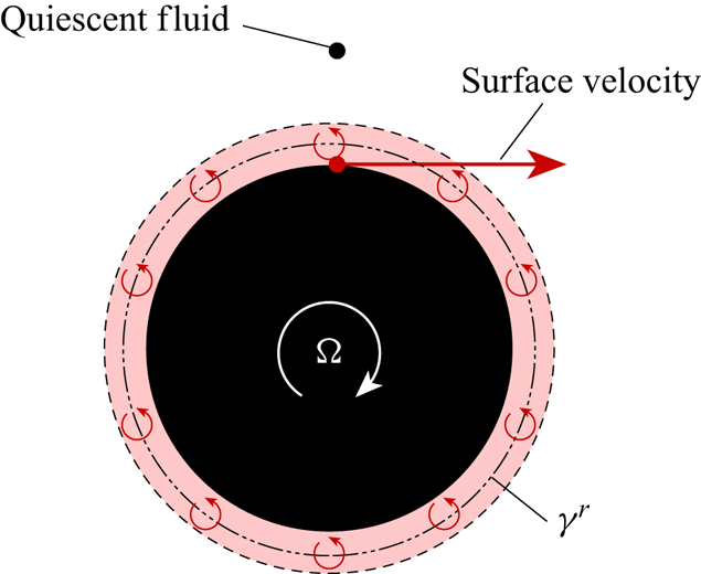
Figure 10. Vortex sheet  $\gamma ^r$ created through cylinder rotation.
To investigate the variation and development of  $\gamma ^b_{sep}$ further, we consider a translating as well as rotating cylinder next.
3.2. Translation and rotation,  $\alpha = 2.5$

The rotation ratio  $\alpha$ is set to 2.5 and the boundary layer vorticity is analysed in the same way as for $\alpha = 0$. The cylinder begins to translate and rotate simultaneously from a stationary start and accelerates until $s/D = 2$. Initially, attached positive vorticity is observed within the entire boundary layer created by the rotary motion. As the cylinder translates further, vorticity detaches all along the downstream surface of the cylinder, with a clear unsteady separation point appearing around $s/D = 1$. The shed vorticity subsequently rolls up into a single vortex which drifts away from the cylinder, as shown in figure 11.

Figure 11. Vorticity contours as the cylinder translates from right to left; (a)  $s/D = 1.0$, (b) $s/D = 2.0$.
Once again the boundary layer vortex sheet is extracted and shown at selected intervals in figure 12, where the line colour shifts from red to blue with increasing translation distance. The separation point is indicated with an equivalently colour coded circle. We observe that  $\gamma ^b$ features a distinctive sinusoidal distribution on the upper cylinder surface and upstream of the separation point. This shape is attributed to the vortex sheet contribution due to motion, $\gamma ^{tr}$, and is similar to that observed earlier for the purely translating cylinder.

Figure 12. Development of  $\gamma ^b$. Circles mark the separation point. Line colour transitions from red to blue with increasing $s/D$.
With increasing  $s/D$ the entire boundary layer vortex sheet distribution ${0 < \theta < 250}$, apart from the region downstream of the separation point, appears to shift downwards almost uniformly. The same is observed for the vortex sheet strength at the separation point, which further demonstrates that the strength of $\gamma ^b$ alone cannot be used to predict the unsteady separation.
3.2.1. Influence of $\gamma ^{shed}$

A change in the boundary layer vortex sheet can only be caused by one of its constituent parts. Since a constant rotation is reached almost instantaneously and the cylinder only accelerates until  $s/D = 2$, the vortex sheet contributions due to translation, $\gamma ^{tr}$, and rotation, $\gamma ^r$, cannot be responsible for the continuing downward drift of $\gamma ^b$. Instead, we propose that this is linked to the behaviour of shed vorticity.
Imagine an external vortex located in close proximity to the cylinder. To calculate its contribution to  $\gamma ^{shed}$, we follow the approach outlined in § 3.1. A mirror image of the external vortex is placed inside the cylinder and the induced velocity from the external and the mirror vortex is found all along the cylinder surface. Assuming that the external vortex is close to the cylinder, we observe that the mirror image vortex is well away from the cylinder centre and relatively close to the surface. This has an important effect on the mirror vortex sheet distribution. Close to the external vortex the induced velocities from either vortex add up, while on the opposite side they tend to roughly cancel; as long as the distance between the surface and the external vortex is small compared to the cylinder diameter. The resulting vortex sheet is therefore confined to the vicinity of the external vortex whilst almost vanishing elsewhere along the cylinder surface, as shown schematically at the top of figure 13. If the external vortex is instead located infinitely far way, a very different effect is observed. Now the mirror vortex is located at the cylinder centre. The induced velocity from the external vortex approaches zero because of the large distance, whilst the mirror image at the cylinder centre induces an equal velocity all along the surface giving a vortex sheet of uniform strength, as shown at the bottom of figure 13. For convenience, we will refer to the vortex sheet contribution due to vorticity in close proximity to the cylinder as $\gamma ^{shed}_{local}$ and to the component from vorticity far away as $\gamma ^{shed}_{far\text {-}field}$.

Figure 13. Effect of local and far-field vorticity.
Effectively, any external vortex contributes to both  $\gamma ^{shed}_{local}$ and $\gamma ^{shed}_{far\text {-}field}$ and the distance from the cylinder simply determines the relative balance between the two components; such that
 \begin{equation} \gamma^{shed} = \gamma^{shed}_{local} + \gamma^{shed}_{far\text{-}field}. \end{equation}
For example, whilst a vortex is close to the cylinder, its local contribution dominates. However, as it drifts away,  $\gamma ^{shed}_{local}$ diminishes and the vortex instead begins to contribute more to the far-field component, as shown in figure 14.
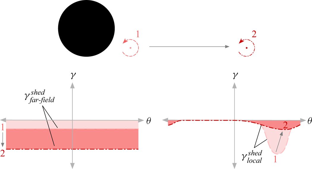
Figure 14. Variation of  $\gamma ^{shed}_{far\text {-}field}$ and $\gamma ^{shed}_{local}$ as a vortex moves away from the cylinder.
The question arises as to how to distinguish between the local and far-field contributions, as the correct attribution is somewhat arbitrary. For instance, setting a cutoff distance after which vorticity is counted as far field rather than as local, to determine its respective contribution to  $\gamma ^{shed}$, introduces an additional unknown in the form of the cutoff distance. Instead, we propose a simple yet more systematic method to estimate the respective distributions. The far-field contribution to the vortex sheet is found by calculating the velocity induced by the external vortex and its mirror image on the opposite side of the cylinder, as schematically illustrated in figure 15. As described earlier, the velocity induced by vorticity in close proximity to the surface will approximately cancel with its mirror image here, whereas this will not occur if vorticity is far away. It follows that $\gamma ^{shed}_{local}$ is the remainder when the far-field contribution, $\gamma ^{shed}_{far\text {-}field}$ is removed from the total vortex sheet due to shed vorticity, $\gamma ^{shed}$,
 \begin{equation} \gamma^{shed}_{local} = \gamma^{shed} - \gamma^{shed}_{far\text{-}field}. \end{equation}
Figure 15. Schematic illustrating the calculation of  $\gamma ^{shed}_{far\text {-}field}$.
The methodology outlined above to estimate  $\gamma ^{shed}_{far\text {-}field}$ is applicable to any shape that can be mapped to a cylinder. For irregular objects, where this is not possible, a panel method approach could be used, where the vortex sheet at position $p_n$ on the cylinder surface created by the $n$th vortex element in the flow field, is matched by the vortex sheet created through a vortex located at infinity.
The total vortex sheet due to vorticity in the flow field,  $\gamma ^{shed}$, normalized by the instantaneous translation velocity, is shown in figure 16(a). Compared to the distribution of the total boundary layer vortex sheet $\gamma ^b$ shown in figure 12, the contribution arising from cylinder translation and rotation $\gamma^{tr + r}$ is removed. Similar to the development of $\gamma ^b$ seen in figure 12, $\gamma ^{shed}$ also displays a downwards drift with increasing translation distance.
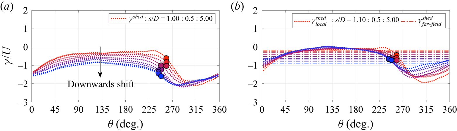
Figure 16. Evolution of (a)  $\gamma ^{shed}$ as well as (b) $\gamma ^{shed}_{local}$ and $\gamma ^{shed}_{far\text {-}field}$. Line colour transitions from red to blue with increasing $s/D$. Circle marks the separation location.
To better understand what is causing this drift,  $\gamma ^{shed}$ is decomposed into its local and far-field contribution in figure 16(b). From this, it becomes apparent that $\gamma ^{shed}_{far\text {-}field}$ is responsible for the observed downwards drift of $\gamma ^{shed}$ and $\gamma ^b$. This makes sense as, with time, shed vorticity moves away from the cylinder and accumulates in the far field, thereby increasing the contribution from $\gamma ^{shed}_{far\text {-}field}$. Interestingly, $\gamma ^{shed}_{local}$ instead remains remarkably invariant as the cylinder translates and in particular its strength at the separation point shows little change.
3.2.2. Scaling the boundary layer vortex sheet strength
In light of the findings regarding the influence of far-field vorticity on the boundary layer vortex sheet, the evolution of  $\gamma ^b$ as well as the development of its strength at the separation point, $\gamma ^b_{sep}$, are revisited. To do so, a new parameter is formed, removing the influence of far-field vorticity and scaling the result with the instantaneous velocity,
 \begin{equation} \bar{\gamma}^b = \frac{\gamma^b - \gamma^r - \gamma^{shed}_{far\text{-}field}}{U}. \end{equation}
Here,  $\gamma ^r$ is also removed, as this is entirely independent of $U$. In other words, $\bar {\gamma }^b$ describes a vortex sheet due to translation $\gamma ^{tr}$ and the effect of vorticity close to the cylinder $\gamma ^{shed}_{local}$,
 \begin{equation} \bar{\gamma}^b = \frac{\gamma^{tr} + \gamma^{shed}_{local}}{U}. \end{equation}
 Figure 17(a) shows that this new vortex sheet strength parameter almost completely collapses the boundary layer vorticity distribution as the cylinder translates. Furthermore, the strength at the separation point also remains much more constant. This is seen more clearly in figure 17(b) where  $\bar {\gamma }^b_{sep}$ is extracted for every time step once separation has been identified. The value of $\bar {\gamma }^b_{sep}$ is compared to $\bar {\gamma }^{b-r}_{sep}$, the equivalent case where $\gamma ^{shed}_{far\text {-}field}$ is retained,
 \begin{equation} \bar{\gamma}^{b-r}_{sep}=\frac{\gamma^b - \gamma^r }{U}. \end{equation}
Whilst  $\bar {\gamma }^{b-r}_{sep}$ shows a clear downwards trend, $\bar {\gamma }^{b}_{sep}$ remains almost invariant.
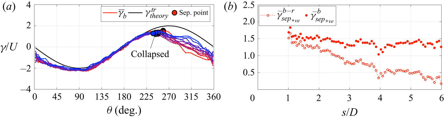
Figure 17. Evolution of (a)  $\bar {\gamma }^b$ between $1 < s/D < 5$ in steps of 0.5, where the line colour changes from red to blue with increasing $s/D$, and (b) the development of $\bar {\gamma }^{b-r}_{sep}$ and $\bar {\gamma }^b_{sep}$. Case 2a.
It may now appear surprising that we did not observe this downwards trend of  $\gamma ^b_{sep}$ for the surging cylinder in figure 9, since vorticity is equally shed. The difference from the rotating case, however, is that vorticity of equal magnitude is shed from either side of the cylinder, creating an approximately symmetric flow field about the $x$-axis running through the cylinder. Since the vorticity released on either side of the cylinder is of opposite sign, the far-field contribution created by the positive and negative vorticity cancels, thus leading to the more constant progression of $\gamma ^b_{sep}$ even before it has been scaled according to (3.9).
Furthermore, the results may offer a possibility to explain the downwards trend observed in the LESP criterion during vortex shedding as reported by Deparday & Mulleners (Reference Deparday and Mulleners2019) and He & Williams (Reference He and Williams2020). The expansion of the velocity singularity around the leading edge by Ramesh (Reference Ramesh2020) links the LESP criterion directly to the leading edge velocity. In potential flow, the boundary layer edge velocity can in turn be straightforwardly linked to the vortex sheet strength used in the present study. Therefore, it may be possible to extrapolate from the results presented in this paper to explain the decline in the LESP strength observed during vortex shedding. This could lead to the tentative conclusion that the reduction in the LESP is caused by more far-field vorticity populating the flow field. This would change the  $A_0$ Fourier coefficient, representative of the LESP, since it has a specific term dedicated to the effect of flow field vorticity. However, a more in-depth study is suggested to confirm this hypothesis.
3.3. Translation and rotation, $\alpha = 1$

In the previous example a single vortex sheds and drifts away, with no further vortex being created during the investigated time period. To test the proposed ideas in a more complex situation, the final example consists of a surging and rotating cylinder at a rotation ratio of 1, where alternate vortices are shed from either side of the cylinder.
The clockwise rotating cylinder initially sheds a single starting vortex from its lower surface which slowly moves away, as seen in figure 18(a,b). Thereafter, a second vortex begins to develop along the upper surface of the cylinder and eventually also advects downstream; this is observed in figure 18(c,d). As the second vortex advects away, a significant change to the vorticity on the lower side of the cylinder is observed. It no longer forms a shear layer which ‘connects’ the starting vortex to the cylinder surface but instead rolls up into a new vortex and thus establishes the commonly observed alternate shedding pattern.

Figure 18. Normalized vorticity contours as the cylinder begins to translate and rotate; (a)  $s/D = 1.0$, (b) $s/D = 2.0$, (c) $s/D = 4.0$, (d) $s/D = 6.5$. Case 2b.
To make the analysis of this unsteady flow field easier, we chose to group the flow into two stages. The ‘development’ period describes the time when the starting vortex is shed from the lower cylinder surface and drifts away, whilst simultaneously a vortex forms along the upper surface, figure 18(a–c). The ‘periodic shedding’ stage describes the flow field when the vortex created along the top surface advects away and at the same time a further vortex forms on the bottom side of the cylinder, figure 18(d).
During the development period,  $\bar {\gamma }^{b-r}$ gradually shifts downwards, as seen in figure 19(a). This coincides with positive vorticity accumulating in the far field, which creates a negative vortex sheet contribution. During the periodic shedding phase, the opposite is observed, as shown in figure 19(c), and $\bar {\gamma }^{b-r}$ moves back upwards. At this point, negative vorticity from the second vortex negates the contribution created by the positive vorticity residing within the starting vortex and thus the overall far-field contribution reduces.

Figure 19. Distribution of  $\gamma ^{b-r}_{sep}$ (a) during the developmental phase $1 < s/D < 4.5$, and (c) during periodic shedding $4.5 < s/D < 7$. Distribution of $\bar {\gamma }^b$ (b,d) at the same time steps. Circles and triangles indicate the separation point; $s/D$ increases in steps of 0.5 as the line colour changes from red to blue, Case 2b.
The ‘corrected’ distribution,  $\bar {\gamma }^{b}$, is shown in figures 19(b) and 19(d). Accounting for the effect of far-field vorticity, and excluding its contribution to the boundary layer vortex sheet, removes the overall drift of $\bar {\gamma }^{b}$ and causes it to collapse throughout the two time periods.
3.4. Comparison of vortex sheet strength at separation
To visualize and highlight the effect that different kinematic motions and external far-field vorticity have on the boundary layer vortex sheet strength at the separation point, we compare the raw value  $\gamma ^b_{sep}$ to its corrected counterpart $\bar {\gamma }^b_{sep}$ for all three cases.
From figure 20(a) it is immediately obvious that the uncorrected vorticity at the separation point is not always the same, that in some cases it varies considerably with  $s/D$, and that there is no critical value that could predict unsteady flow separation. However, when the effects of rotation rate, far-field vorticity and instantaneous velocity are accounted for, the resulting boundary layer vortex sheet parameter $\bar {\gamma }^b_{sep}$ collapses very well to an almost constant level, as shown in figure 20(b). Only $\bar {\gamma }^b_{sep}$ along the bottom surface of Case 2 (upright red triangles in figure 20b) slightly deviates from this trend at around $s/D = 5$, which coincides with the emergence of a second vortex shedding from the lower cylinder surface.

Figure 20. Development of (a) the raw boundary layer vortex sheet strength at the separation point  $\gamma ^{b}_{sep}$ and (b) the new boundary layer vortex sheet parameter $\bar {\gamma }^b_{sep}$, for all cases.
4. Conclusion
The development of the boundary layer vorticity during unsteady flow, containing body acceleration as well as large scale separation, is explored experimentally by translating and rotating a circular cylinder in a quiescent fluid. By combining time-resolved velocity data with a potential flow analysis, the boundary layer can be represented by a vortex sheet distribution which contains a number of contributions that can be attributed to different physical effects, namely translation, rotation, near-field and far-field vorticity.
Translation creates a boundary layer vortex sheet component that can be calculated from the potential flow solution and can be experimentally recovered for bodies of volume in real viscous flow featuring substantial external vorticity. Rotation leads to a further contribution resulting from the slip velocity between the cylinder surface and the surrounding quiescent flow. External vorticity also contributes to the boundary layer vortex sheet by creating a mirror image that is equal and opposite in magnitude and is distributed over the cylinder surface. It is proposed that the vortex sheet component from external vorticity can be decomposed into a ‘local’ and ‘far-field’ contribution. Vorticity close to the cylinder creates a vortex sheet component that acts only on a small, local portion of the cylinder surface, whilst the far-field component provides a uniform contribution everywhere.
The evolution of the cylinder boundary layer vortex sheet can therefore be explained by the development of these respective vortex sheet components. The growth, decline or shift of the boundary layer vortex sheet can be deconstructed and traced back to a number of simple phenomena, thereby no longer appearing arbitrary. As such, acceleration will cause the vortex sheet to grow, whereas accumulation of vorticity far away from the cylinder will create an oppositely signed vortex sheet contribution all along the cylinder surface. By accounting for these mechanisms, the resulting vortex sheet remains largely invariant throughout the cylinder motion and for a variety of kinematic cases.
Evaluating the behaviour of the boundary layer vortex sheet strength at the unsteady separation point can further explain why others have found boundary layer vorticity, evaluated directly or indirectly, a useful tool when analysing unsteady separation but also why it has been difficult to find a universally valid threshold in terms of vorticity to predict separation. Removing the vortex sheet contributions due to rotation, far-field vorticity and accounting for instantaneous velocity, yields a dimensionless vortex sheet strength at the separation point that appears to be independent of kinematics and time. This persists for as long as no repeated vortex shedding occurs from the same side of the cylinder. The result may explicitly or implicitly enable the prediction of the unsteady separation point. In contrast, the raw strength of the boundary layer vortex sheet cannot be used to indicate unsteady separation, as significant variations of its strength at the unsteady separation point are observed.
Funding
The authors would like to acknowledge the Engineering and Physical Science Research Council (EPSRC) for providing financial support, EP/M508007/1 and EP/N509620/1.
Declaration of interests
The authors report no conflict of interest.


 Open access