


1. Introduction
The flow past a circular cylinder is a classical configuration which has been widely adopted in the fluid dynamics community as a canonical model to investigate vortex shedding behind bluff bodies. In the case of a fixed cylinder, i.e. without rotation, the dynamics and the corresponding bifurcations are well known (Williamson Reference Williamson1996). The case of a rotating cylinder, which has implications for flow control using wall motion (Modi Reference Modi1997; el Hak Reference el Hak2000), has recently received attention. A number of numerical studies in a two-dimensional framework have been conducted (Kang, Choi & Lee Reference Kang, Choi and Lee1999; Stojković, Breuer & Durst Reference Stojković, Breuer and Durst2002, Reference Stojković, Breuer and Durst2003; Mittal Reference Mittal2004) and have revealed the existence of several steady and unsteady regimes. Linear stability approaches (Pralits, Brandt & Giannetti Reference Pralits, Brandt and Giannetti2010; Pralits, Giannetti & Brandt Reference Pralits, Giannetti and Brandt2013) have shown the existence of two separated regions of instability in the  $(Re,\alpha )$ plane, where $\alpha$ is the dimensionless rotation rate and $Re$ is the Reynolds number. The so called Mode I becomes unstable via a supercritical Hopf
bifurcation and it is present for  $0 \leq \alpha \leq 2$. This mode is the one associated with the classical Bénard–von-Kármán vortex street, and characterised by the alternate shedding of vortices of opposite sign. At higher rotation rates, around $4.5 \leq \alpha < 6$ another unsteady mode exists, denoted as Mode II. The physical mechanism driving this mode is rather different, as it corresponds to a slow-frequency shedding of vortices with the same vorticity sign. Its onset is less well characterised than Mode I from the point of view of bifurcation theory: the fact that the frequency is very low suggests a more complex bifurcation scenario and its supercritical or subcritical nature is still unclear. The full characterisation of Mode II is complicated by the fact that, in approximately the same range of $(Re,\alpha )$ parameter space, a region where three steady-state solutions coexist has been evidenced (Pralits et al. Reference Pralits, Brandt and Giannetti2010; Rao et al. Reference Rao, Leontini, Thompson and Hourigan2013a). A more thorough characterisation of this phenomenon has been carried out by Thompson et al. (Reference Thompson, Rao, Leontini and Hourigan2014) who observed that the region of existence of multiple steady-state solutions grows with the Reynolds number. Note also that the picture is further complicated by the existence of three-dimensional (3-D) instabilities in this range. This point is outside of the range of the present paper which restricts to 2-D dynamics, but a brief review on 3-D stability properties of this flow can be found in appendix E.
To explain the existence of multiple steady states, Rao et al. (Reference Rao, Leontini, Thompson and Hourigan2013a) conjectured that they emerge from a cusp bifurcation point. Indeed, a cusp correctly explains the change in the number of steady states from one to three. However, a cusp is not generally associated with the existence of a Hopf bifurcation in the same range of parameters, so it cannot explain, alone, all the features discussed above. The fact that the frequency of Mode II is very small is an indicator of a second kind of codimension-two bifurcation, namely a  $0^2$ or Takens–Bogdanov bifurcation (Kuznetsov Reference Kuznetsov2013, chapter 8, p. 314) This bifurcation typically occurs when the frequency of a limit cycle vanishes. However, in the vicinity of a standard Takens–Bogdanov bifurcation, only two steady states generally exist, not three. This combination of features suggests that the picture could hide a codimension-three bifurcation point, also known as a generalised Hopf bifurcation. The unfolding of this generalised Takens–Bogdanov bifurcation has been studied by Dumortier et al. (Reference Dumortier, Roussarie, Sotomayor and Zoladek2006) and Kuznetsov (Reference Kuznetsov2005) from a mathematical point of view, but to our knowledge such a feature has not yet been evidenced in a fluid dynamics system such as the one considered here.
The main purpose of the present work is to review the classification of the possible 2-D states in the  $(Re,\alpha ) \in [0 , 200] \times [0,10]$ parameter plane with the point of view of dynamical system theory. Firstly, we will characterise the nature of the codimension-one bifurcation curves (Hopf or saddle nodes). We give a cartography of the regions where multiple steady states exist and give a detailed description of these multiple states as well as their stability properties. We further identify three codimension-two points, namely a Takens–Bogdanov (TB) bifurcation, a cusp and a generalised Hopf (GH) bifurcation. We show that the two first are effectively located very close to each other and that the whole dynamics in this range of parameters is effectively described by the unfolding of a codimension-three bifurcation point.
The article is organised as follows: in § 2 the formulation of the problem is discussed together with the methodology adopted in the present analysis. Section 3 begins with a characterisation of the multiple steady states. A complete bifurcation diagram covering the range  $(Re,\alpha ) \in [ 0,200 ]\times [0,10]$ is then presented. The next subsections aim at clarifying the picture in the vicinity of the identified codimension-two points.
2. Problem formulation and investigation methods
2.1. Geometrical configuration and general equations
The two-dimensional flow past a rotating circular cylinder is controlled by two parameters: the Reynolds number  $Re= {U_\infty D}/{\nu }$ and the rotation rate $\alpha = {\varOmega D}/{2 U_\infty }$. Here, $\varOmega$ is the dimensional cylinder angular velocity, $U_{\infty }$ is the free stream velocity, $D$ the diameter of the cylinder and $\nu$ the dynamic viscosity of the fluid. The fluid motion inside the domain is governed by the two-dimensional incompressible Navier–Stokes equations,
 \begin{gather} \frac{\partial \boldsymbol{U}}{\partial t} + \boldsymbol{U} \boldsymbol{\cdot} \boldsymbol{\nabla}\boldsymbol{U} = -\boldsymbol{\nabla} P + \boldsymbol{\nabla} \boldsymbol{\cdot} \tau(\boldsymbol{U} ), \end{gather}
 \begin{gather}\boldsymbol{\nabla} \boldsymbol{\cdot} \boldsymbol{U} = 0, \end{gather}
where  $\boldsymbol {U}$ is the velocity vector whose components are $(U,V)$, $P$ is the reduced pressure and the viscous stress tensor $\tau (\boldsymbol {U})$ can be expressed as $\nu (\boldsymbol {\nabla } \boldsymbol {U} + \boldsymbol {\nabla } \boldsymbol {U}^\textrm {T})$. The incompressible Navier–Stokes equations (2.1) are complemented with the following boundary conditions: on the cylinder surface, no-slip boundary conditions are set by $\boldsymbol {U} \boldsymbol {\cdot } \boldsymbol {t} = \varOmega D/2$ and $\boldsymbol {U} \boldsymbol {\cdot } {\boldsymbol {n}} = 0$, where $(\boldsymbol {t}, \boldsymbol {n})$ are the director vectors of the surface in the plane ( $x,y$); in the far field, uniform boundary conditions are set $U \rightarrow (U_\infty , 0)$ when $r \rightarrow \infty$, where $r$ is the distance to the cylinder centre (see figure 1). In the discussion we consider clockwise rotation of the cylinder surface ( $\alpha >0)$.
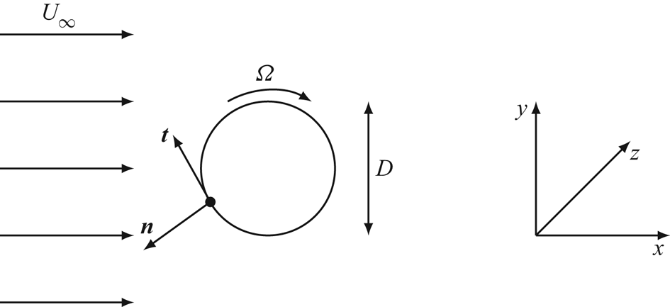
Figure 1. Sketch of a rotating cylinder immersed in a uniform flow.
In the following, Navier–Stokes equations (2.1) and the associated boundary conditions will be written symbolically under the form  ${\mathcal {B}} ({\partial \boldsymbol {Q}}/{\partial t}) = {\mathcal {N}S}(\boldsymbol {Q})$, where $\boldsymbol {Q} = (\boldsymbol {U},{P})$ is the state vector and ${\mathcal {B}}$ is a linear projection operator, meaning that the time derivatives apply only on the velocity components.
2.2. Linear stability analysis
Under the framework of linear stability analysis, we first need to identify base-flow solutions defined as the steady solutions  $\boldsymbol {Q}_b$ of the (two-dimensional) Navier–Stokes equations, namely the solutions of ${\mathcal {NS}}(Q_b) = 0$. We then characterise the dynamics of small-amplitude perturbations around this base flow by expanding them over the basis of linear eigenmodes, i.e.
 \begin{equation} \boldsymbol{Q}(x,y,t) = \boldsymbol{Q}_b(x,y) + \epsilon \sum_j \hat{\boldsymbol{q}}_j(x,y) \exp(\lambda_j t). \end{equation}
Here,  $\epsilon$ is a small parameter, $\lambda _j$ the eigenvalues and $\hat {\boldsymbol {q}}_j$ the eigenmodes. The eigenpairs $[\lambda _j, \hat {\boldsymbol {q}}_j]$ have to be determined as the solutions of the following eigenvalue problem:
 \begin{gather} \lambda \hat{\boldsymbol{u}} + \boldsymbol{u}_b\boldsymbol{\cdot} \boldsymbol{\nabla} \hat{\boldsymbol{u}} + \hat{\boldsymbol{u}}\boldsymbol{\cdot}\boldsymbol{\nabla} \boldsymbol{u}_b = - \boldsymbol{\nabla} \hat{p} + \boldsymbol{\nabla} \boldsymbol{\cdot} \tau({\hat{\boldsymbol{u}}}) \end{gather}
 \begin{gather}\boldsymbol{\nabla} \boldsymbol{\cdot} {\hat{\boldsymbol{u}}}= 0. \end{gather}
Which will be written in the following under the symbolic form  $\lambda _j {\mathcal {B}} \hat {\boldsymbol {q}}_j + {\mathcal {LNS}} \hat {\boldsymbol {q}}_j = 0$. In the following we consider that eigenmodes ${\hat {\boldsymbol {q}}}(x,y)$ have been normalised, see appendix C for further details. Note that in (2.2), to fully represent the dynamics, the summation over eigenmodes may involve a continuous sum over the spectrum, i.e. the discrete and the continuous or essential spectra of the operator (see Kapitula & Promislow (Reference Kapitula and Promislow2013) for a rigorous discussion). However, to determine global stability we only need to consider a limited number of eigenmodes, so we keep the summation as a discrete sum indexed by $j$.
$j$.
Owing to the eigenvalues, two cases can be distinguished:
(i) If all eigenvalues $\lambda _j$ have negative real part the considered base flow is a stable solution.
(ii) If
$n$ eigenvalues have positive real part, the considered base flow will be referred to as a $n$-unstable solution. Note that 1-unstable solutions are commonly referred to as saddle points because a projection of their dynamics in a 2-D plane (phase portrait) has an attractive direction and another repulsing one, while 2-unstable solutions are either unstable nodes or unstable foci depending if the leading eigenvalues are both real or complex conjugates.


The transition from stable to unstable (or from  $n$-unstable to $n+1$-unstable) is called a local bifurcation. The simplest bifurcations (such as saddle nodes and Hopf) are said to be codimension-one and occur along given curves in the parameter plane ( $Re,\alpha$). The intersection of two such curves tangentially is called a codimension-two bifurcation and generally leads to a rich dynamics in the vicinity of the intersection point.
2.3. Notions of bifurcation theory
From the viewpoint of dynamical system theory, the expression (2.2) can be generalised as a decomposition of the perturbations over the leading modes of the system
 \begin{equation} \boldsymbol{Q}(x,y,t) = \boldsymbol{Q}_b(x,y) + \sum_j A_j(t) \hat{\boldsymbol{q}}_j(x,y). \end{equation}
Then, the problem can be reduced to a low-dimensional system governing the amplitudes  $A_j(t)$
 \begin{equation} \frac{\textrm{d}}{\textrm{d}t} A_j = \lambda_j A_j + (NL), \end{equation}
where  $(NL)$ represent the nonlinear interactions between modes. Investigation of these nonlinear terms allows us to predict the dynamics in the vicinity of bifurcation points. Systematic methods exist to compute these nonlinear terms (such as weakly nonlinear expansions, centre manifold reduction or Lyapunov–Schmidt reduction). However, restricting ourselves to a qualitative point of view (up to a continuous change of coordinates with continuous inverse), it is also possible to predict a number of features by examining the generic normal form of the bifurcation, namely, a standard form to which the dynamical system can be reduced by a series of elementary manipulations (see Wiggins (Reference Wiggins2003) for details). Particular forms of codimension-two bifurcations encountered in the rotating cylinder are discussed in §§ 3.5 and 3.6.
2.4. Numerical methodology
In the present manuscript, we adopt the same numerical methodology used in Fabre et al. (Reference Fabre, Longobardi, Citro and Luchini2020) and described in Fabre et al. (Reference Fabre, Citro, Sabino, Ferreira, Sierra, Giannetti and Pigou2019). The computation of the steady-state solutions, the resolution of the linear problems and the time stepping techniques are implemented using the open-source finite element software FreeFem++. Parametric studies and generation of figures are performed using Octave/Matlab thanks to the generic drivers of the StabFem project (see a presentation of these functionalities in Fabre et al. Reference Fabre, Citro, Sabino, Ferreira, Sierra, Giannetti and Pigou2019). According to the philosophy of this project, codes reproducing parts of the results of the present paper are available from the StabFem website (https://gitlab.com/stabfem/StabFem). On a standard laptop, all the computations discussed below can be obtained in a few hours, except time stepping simulations which take longer. Results presented in § 3 are obtained with a computational domain  $L_x = 120$ and $L_y = 80$ in the streamwise and cross-stream directions, respectively. The cylinder centre is located $40$ diameters downstream of the inlet, symmetrically between the top and bottom boundaries. Numerical convergence issues are discussed in appendix D by a meticulous comparison between results obtained with different meshes, where domain dimension and grid density were varied.
Steady nonlinear Navier–Stokes equations are solved by a Newton method. In the degenerated cases, pseudo-arc length continuation is performed to be able to compute multiple steady-state solutions, as described in appendix A. The generalised eigenvalue problem (2.3) is solved by the Arnoldi method or by a simple inverse iteration algorithm. Finally, nonlinear unsteady Navier–Stokes equations are integrated forward in time with a second-order time scheme (Jallas, Marquet & Fabre Reference Jallas, Marquet and Fabre2017).
3. Results
3.1. Characterisation of multiple steady-state solutions
To introduce the existence of multiple steady states, we first characterise them by plotting in figure 2 the associated lift as function of the rotation rate  $\alpha$, for four different values of $\alpha$. In these plots, stable solutions are indicated by continuous lines and unstable ones by dashed lines, following the usual convention in dynamical systems theory.
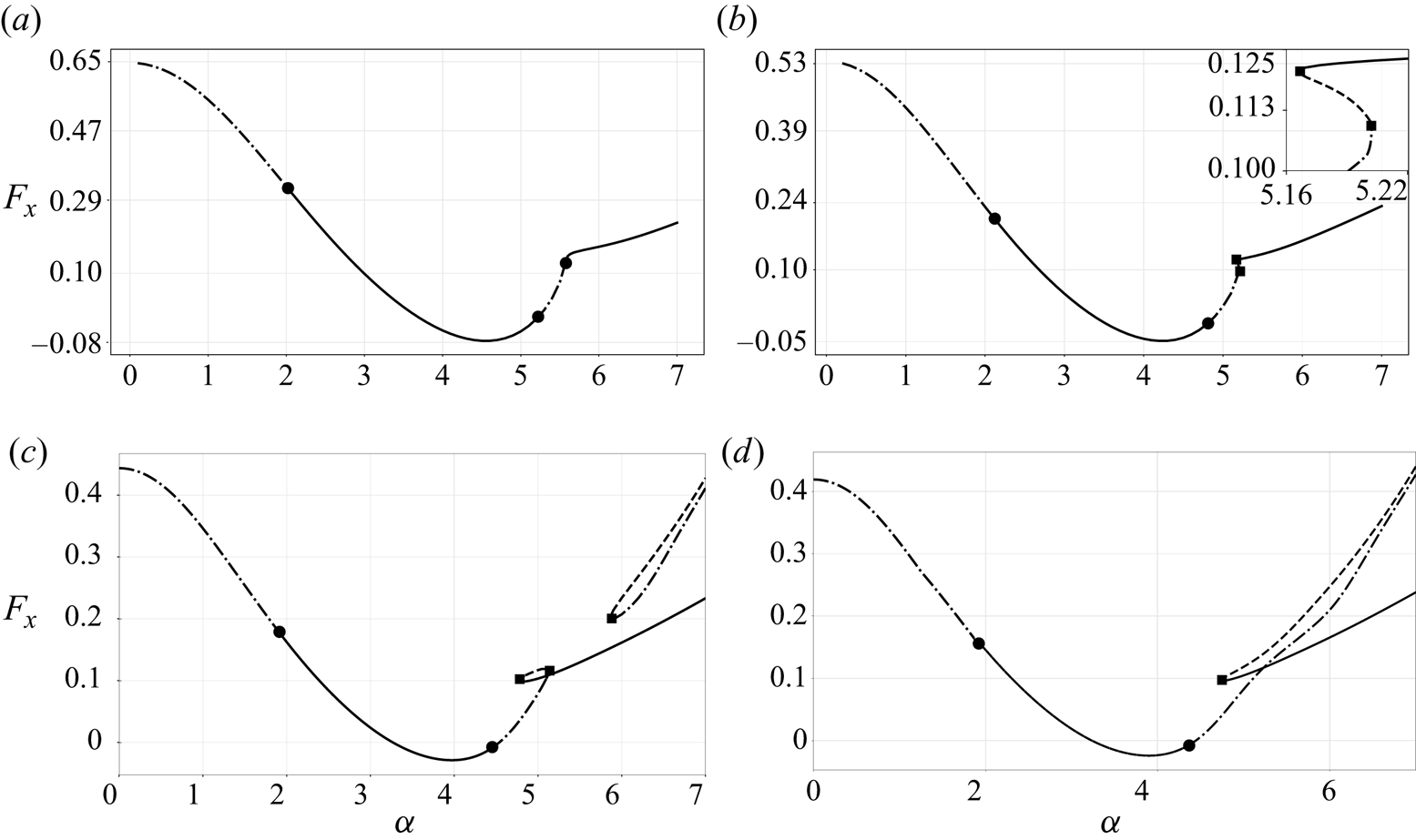
Figure 2. Evolution of the horizontal force  $F_x$ as a function of the rotation rate $\alpha$ for four Reynolds numbers, (a) $Re=60$, (b) $Re=100$, (c) $Re=170$ and (d) $Re=200$. Solid lines
 ![]() denote stable steady states, dashed-dotted lines
denote stable steady states, dashed-dotted lines ![]() denote unstable steady states of focus type or nodes, dashed lines
denote unstable steady states of focus type or nodes, dashed lines ![]() are used for steady states of saddle type. Solid circles
are used for steady states of saddle type. Solid circles  denote Hopf bifurcations and solid squares
  denote saddle-node bifurcations.
For  $Re =60$, as illustrated in figure 2(a), only one steady state exists for all values of $\alpha$, for $Re = 60$. This state is stable except in the ranges $\alpha \lesssim 2$ (corresponding to the existence of Mode I), and $5.2 \lesssim \alpha \lesssim 5.5$ (corresponding to the existence of Mode II).
For higher Reynolds numbers, a small region of multiple solutions arises in a small-scale interval around  $\alpha \approx 5$. This phenomenon is illustrated in figure 2(b) for $Re = 100$ and is associated with an ‘s’ shape of the curve, featuring two successive folds. Note that, before the first fold, the steady solution is 2-unstable (focus type); at the first fold it turns into 1-unstable (saddle type) and at the second fold it turns into stable. To detect these folds, pseudo-arc length continuation is carried out with $\alpha$ as a parameter and the horizontal force exerted on the cylinder surface $F_x$ as a monitor to track and distinguish multiple steady states (see appendix A for a more detailed discussion).
For larger values of the Reynolds number, as illustrated in figure 2(c) for  $Re = 170$, the interval of existence of multiple states for $\alpha \approx 5$ expands to $\alpha \in [4.75,5.12]$. In addition, we observe a second range displaying multiple states for $\alpha > 5.87$. This second interval is associated with a fold bifurcation at $\alpha =5.87$, giving rise to two additional and disconnected steady solutions. Note that both these solutions are unstable, respectively of node and saddle types.
Finally, for  $Re=200$, as illustrated in figure 2(d), we observe that the two ranges of multiple steady states are merged into a single one. In this case there is a single saddle-node bifurcation around $\alpha =4.75$ leading to two branches of steady states which are disconnected from the branch existing for lower values of $\alpha$. Here, one of these branches is stable and the second is unstable (saddle type).
3.2. Topological description of steady-state solutions
We now illustrate the spatial structure of some steady-state solutions, with emphasis on the topological structure of the corresponding flows. We restrict ourselves to the case  $Re = 200$, as previously considered in figure 2(d).
Figure 3(a) corresponds to  $\alpha = 1.8$, the value at which Mode I is re-stabilised. The corresponding flow is characterised by a stagnation point located beneath the cylinder axis, on the left side of the $y$-cylinder axis. Compared to the steady flow in the non-rotating case, which is characterised by a symmetrical recirculation region, the upper recirculating bubble is reduced whereas the lower one is moved downwards.
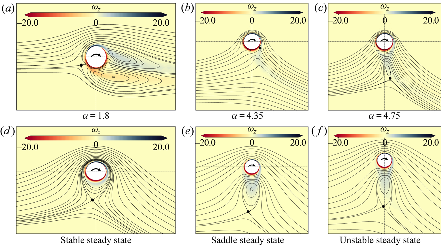
Figure 3. Steady flow around a rotating cylinder (vorticity levels and streamlines) for selected parameters. (a)  $\alpha =1.8,Re= 200$ (at the supercritical Hopf bifurcation threshold); (b) $\alpha =4.35,Re = 200$ (at the Hopf bifurcation); (c) $\alpha =4.75, Re=200$ (at the fold bifurcation). (d–f) Correspond to three base-flow solutions existing in the range of multiple solutions, namely for $\alpha =5.25$ and $Re=200$. The circled dot shows the position of the hyperbolic stagnation point.
Further increasing the rotation speed, both recirculation bubbles shrink and eventually vanish. At  $\alpha = 4.35$ (figure 3b) corresponding to the lower threshold for the existence of Mode II, recirculating bubbles have already disappeared and the vorticity wraps the cylinder. Stagnation point is located on the opposite side but downstream the cylinder vertical axis.
Figure 3(c) corresponds to the steady-state flow at the fold bifurcation observed for  $\alpha = 4.75$ and giving rise to the disconnected states observed in figure 2(d). Compared to the previous state, the flow is topologically different as no stagnation point is observed along the wall of the cylinder. On the other hand, two stagnation points are observed within the flow. One of them is elliptic and located at the centre of the detached recirculation bubble. The other is hyperbolic and located along the streamline bounding the recirculation bubble.
Figure 3(d–f) displays the three coexisting steady states at  $\alpha = 5.25$ and $Re=200$. The topology of the streamlines of unstable and stable steady states differs. In the stable case (panel $d$) there is a single recirculation region encircling the cylinder and bounded by a hyperbolic stagnation point, as in the classical potential solution existing in this range of rotation rates. On the other hand, for both unstable states, the topology is similar to the case of figure 3(c). The recirculation region is detached from the cylinder and contains an elliptic stagnation point located approximately in the midpoint between the hyperbolic point and the bottom point of the cylinder surface. In the unstable steady state, the recirculating region is more stretched, as it can be seen in figure 3(d–f).
We highlight that even though topological changes in the streamlines of the steady states and bifurcations of the velocity field are in general independent events (see Brøns Reference Brøns2007), in some cases these two events occur in a small neighbourhood of the space of parameters (see Heil et al. Reference Heil, Rosso, Hazel and Brøns2017). In the current situation it has been confirmed that there is not a one-to-one relation between both phenomena. For instance, the transition between detached recirculation bubble (as in panel  $c$) and recirculation bubble encircling the cylinder (as in panel $d$) along the stable branch occurs at some value of $\alpha$ in the range $[4.75\text {--}5.25]$ where no dynamical bifurcation occurs. Yet, for larger Reynolds numbers, i.e. $Re \gtrapprox 190$, successive creation and destruction of vortices seems to be relevant in the preservation of the disconnected branch of steady states.
3.3. Analysis of the spatial structure of direct and adjoint eigenmodes
To explain why the steady state displayed in figure 3(f) is unstable, the two corresponding unstable modes (both associated with real eigenvalues) are displayed in figure 4 for  $Re = 200$ and $\alpha = 5.25$. Direct modes are characterised by two recirculating regions of opposite vorticity. Vorticity is stronger and more localised in Mode IIa while Mode IIb displays a larger region with non-zero vorticity. Adjoint eigenvectors $\hat {{\boldsymbol {q}}}^\dagger$ for Mode IIa and Mode IIb are also displayed in figure 4. Adjoint fields (Luchini & Bottaro Reference Luchini and Bottaro2014) can be interpreted as a kind of Green's function for the receptivity of the global mode. Scalar product of the adjoint field with a forcing function or an initial condition provides the amplitude of the instability mode (see Giannetti & Luchini Reference Giannetti and Luchini2007). Therefore, Mode IIa is highly receptive in the upper right side of the near wake of the cylinder. The region of maximum receptivity extends from the close upper right region of the cylinder to a larger region at the bottom right of the cylinder and it is weaker than Mode IIa. Both modes present weak sensitivity to forcing upstream of the cylinder.
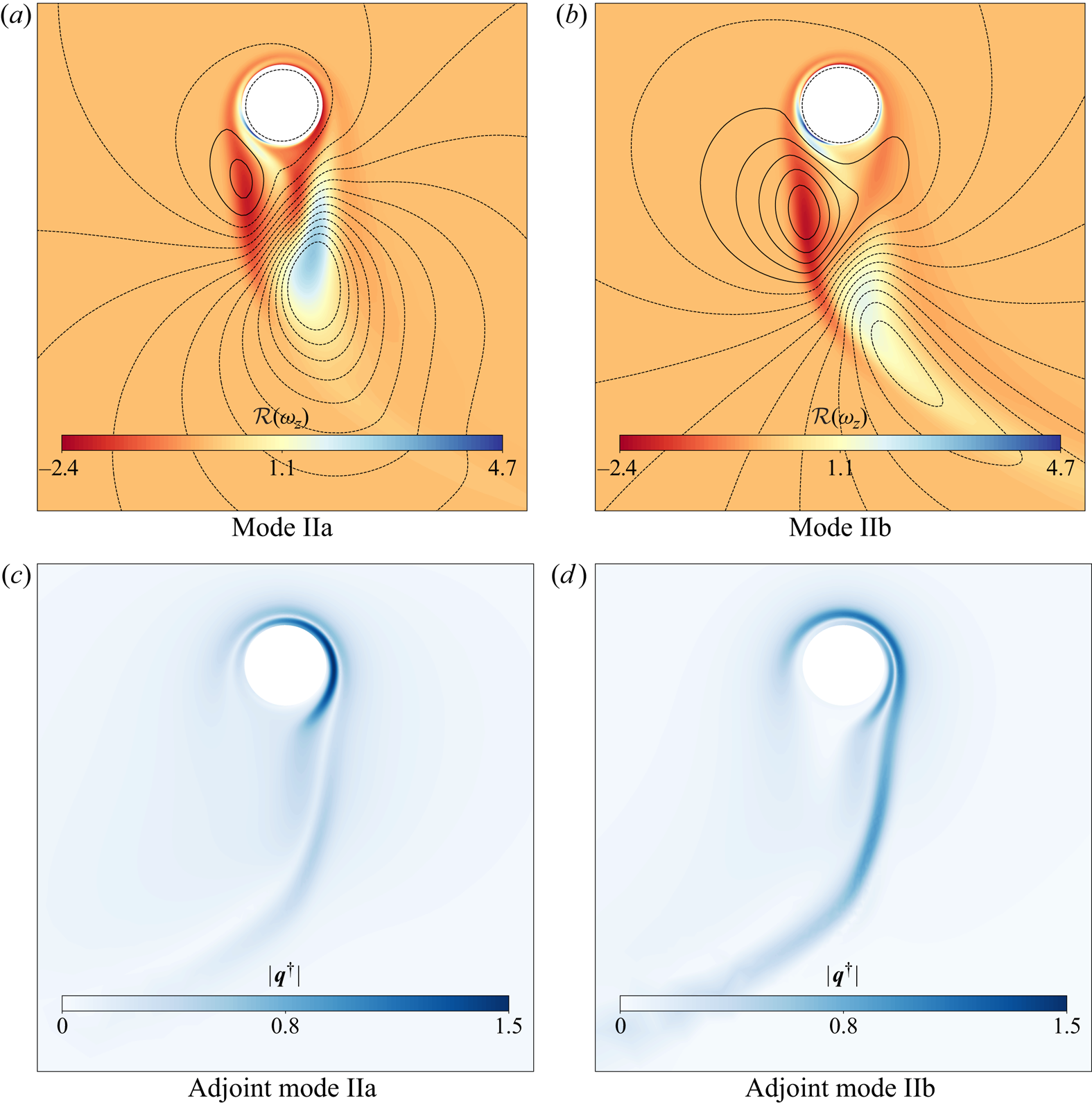
Figure 4. Contour plot of vorticity  $\omega _z$ of Mode IIa and Mode IIb at $\alpha =5.25$ and $Re=200$ of the unstable steady state (a,b). The magnitude of adjoint modes (c,d).
3.4. Bifurcation diagram in the parameter plane $(Re,\alpha$)

The bifurcation curves detected in the  $\alpha <10 ,Re < 200$ range by linear stability analysis of all steady-state solutions are depicted in figure 5.
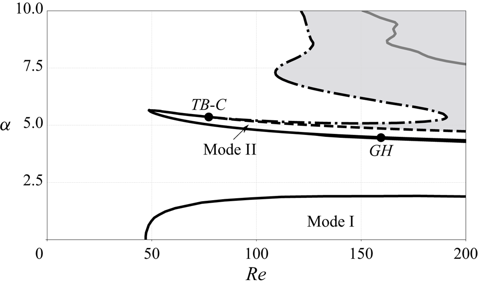
Figure 5. Bifurcation curves in the range  $Re \in [0,200]$ and $\alpha \in {[ 0,10 ]}$. Black and grey lines are used to denote local bifurcations. Solid lines
 ![]() indicate the presence of a Hopf bifurcation, dashed line
indicate the presence of a Hopf bifurcation, dashed line ![]() designates the first fold bifurcation curve,
designates the first fold bifurcation curve,  $F_-$, and dashed dotted line
 ![]() denotes the second fold bifurcation,
denotes the second fold bifurcation,  $F_+$. Grey region indicates the coexistence of three steady states. Solid grey line inside the grey region denotes a secondary Hopf bifurcation occurring on one of the unstable steady states.
Three Hopf bifurcation curves are detected and plotted with full lines. The first one encircles the range of existence of unsteady Mode I. The second one delimits the range of existence of unsteady Mode II in its lower and left parts, but not on its upper part. The third one (in grey) occurs along a steady state which is already unstable, and hence is not likely to be related to a bifurcation observable in DNS or experiments.
In addition, we have identified two bifurcation curves associated with saddle nodes or ‘folds’, here denoted  $F_{+}$ and $F_{-}$. These curves delimit the range of existence of multiple two-dimensional steady states, displayed as a grey region in figure 5. Note that the extension of this region explains the difference between the cases $Re = 170$ and $Re = 200$ discussed in the previous paragraph; according to the figure a single interval of $\alpha$ is found for $Re \gtrsim 190$.
In figure 5, the two fold curves seem to merge with the Hopf curve existing for lower  $Re$ at a point with coordinates $Re \approx 75$, $\alpha \approx 5.4$. Inspection shows that there are actually both a $0^2$ or TB bifurcation and a cusp (C) bifurcation in very close vicinity in this range of parameters. This region will be studied in § 3.5. Additionally, in another range of parameters located at the lower threshold of existence of the Mode II, we have identified the existence of a Bautin or GH bifurcation which splits the Hopf curve into supercritical ( $Re < Re_{GH}$) and subcritical ( $Re > Re_{GH}$). This region will be studied in § 3.6.
3.5. Cusp–Takens–Bogdanov region
3.5.1. Qualitative study of the normal form
The transition occurring for  $Re \approx 75$ and $\alpha \approx 5.4$ is characterised by the end of the Hopf curve ( $H_{-}$) at a fold curve $(F_{+})$ (characteristic of a Takens–Bogdanov bifurcation), and a transition between one and three steady states (characteristic of a cusp). This suggests that the present situation is actually very close to a codimension-three bifurcation. The dynamical behaviour of the system can thus be expected to be well predicted using the normal form describing the universal unfolding of the codimension-three planar bifurcation, also called a generalised TB bifurcation. This normal form has been studied by both Dumortier et al. (Reference Dumortier, Roussarie, Sotomayor and Zoladek2006) and Kuznetsov (Reference Kuznetsov2013, chapter 8.3). The normal form can be written as follows:
 \begin{gather} \frac{\textrm{d} y_1}{\textrm{d} t} = y_2, \end{gather}
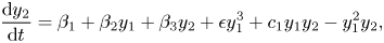 \begin{gather}\frac{\textrm{d} y_2}{\textrm{d} t} = \beta_1 + \beta_2 y_1 + \beta_3 y_2 + \epsilon y_1^3 + c_1 y_1 y_2 - y_1^2y_2, \end{gather}
where  $\beta _1, \beta _2$ and $\beta _3$ are unfolding parameters (mapped from the physical parameters ( $Re,\alpha$)), $c_1$, $\epsilon$ (which can be rescaled to ${\pm }1$) are fixed coefficients which depend on the nonlinear terms of the underlying system. Note that this normal form generalises both the normal form of the standard TB bifurcation (which is recovered for ${\beta _1(Re,\alpha ) = 0}$) and the one of the fold bifurcations (which is recovered for $\beta _3(Re,\alpha ) = 0$). The occurrence of both these codimension-two conditions for very close values of the parameters is characteristic of an imperfect codimension-three bifurcation and justifies the relevance of the associated normal form.
The dynamics of the normal form (3.1) has been explored by Dumortier et al. (Reference Dumortier, Roussarie, Sotomayor and Zoladek2006) who classified the possible phase portraits and the associated bifurcation diagrams as functions of the unfolding parameters  $(\beta _1,\beta _2,\beta _3)$ along a spherical surface. They showed that all possible bifurcation diagrams fall into three possible categories, called focus, saddle and node according to the values of the coefficients $c_1$ and $\epsilon$. The situation $0 < c_1 < 2\sqrt {2}$ and $\epsilon = -1$ corresponds to the stable focus case and is found to lead to a bifurcation diagram consistent with the present situation, so we concentrate on this case.
Figure 6 illustrates all the possible behaviours of the dynamical system, sketched by sample phase portraits, along with their range of existence in the  $(\beta _1,\beta _2)$ plane. This figure corresponds to a subset of the complete diagram displayed in Dumortier et al. (Reference Dumortier, Roussarie, Sotomayor and Zoladek2006, chapter 1, pp. 6–8), restricted to a range of parameters which is sufficient to explain all the dynamical features of the present problem. The bifurcation diagram displays two codimension-two points, a cusp C and a TB. These codimension-two points result from the tangential intersection of two codimension-one curves: the cusp point C occurs when the two fold curves $F_+$ and $F_{-}$ collide, while the TB point arises from the intersection of the supercritical $H_{-}$ Hopf curve and the $F_{+}$ fold. In addition, the bifurcation diagram predicts a homoclinic global bifurcation along a curve $H_{\infty }$ originating from the TB point and terminating along the $F_{-}$ fold on a point denoted SNL (for saddle-node loop). Left from this point, the $F_{-}$ curve corresponds to a local saddle node while right from this point it corresponds to a homoclinic saddle-node bifurcation (appearance of two fixed points along a previously existing cycle). Note that the SNL point and the intersection of $H_{-}$ and $F_{-}$ are formally not codimension-two points (see Dumortier et al. Reference Dumortier, Roussarie, Sotomayor and Zoladek2006).
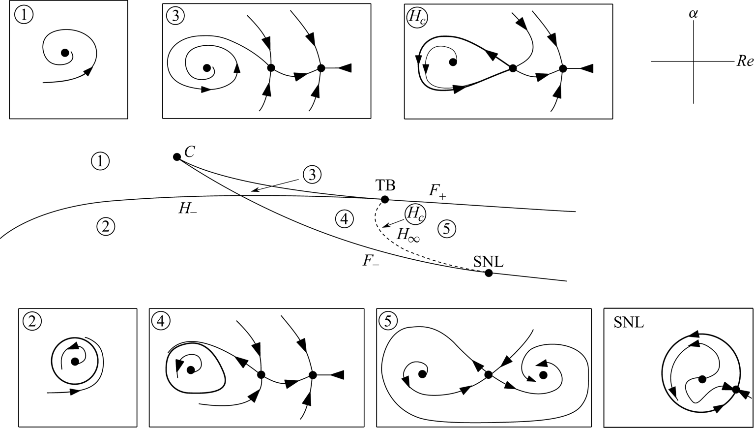
Figure 6. Bifurcation diagram predicted using the normal form 3.1 in the stable focus case (adapted from Dumortier et al. Reference Dumortier, Roussarie, Sotomayor and Zoladek2006), and qualitative phase portrait in regions (1), (2), (3), (4), (5) and along curve  $H_\infty$. Note that in the qualitative phase portraits, focus and node points are not distinguished.
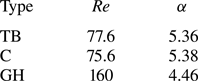
Table 1. Position of codimension-two bifurcation points.
Phase portraits obtained in the various regions delimited by bifurcation boundaries are displayed in the panels of figure 6. One of the most interesting predictions is the existence of two regions characterised by the existence of two stable states, a bistability phenomenon. The first region (3), in the vicinity of the cusp, is characterised by two stable steady states. The third region (4) is characterised by both a stable steady state and a stable cycle. In all other regions, there is a single stable solution which is either a steady state (in regions 1 and 5) or a cycle (in region 2).
Note that in these phase portraits nodes and foci are not distinguished. Distinguishing between these cases (Dumortier et al. Reference Dumortier, Roussarie, Sotomayor and Zoladek2006) leads to consideration of a larger number of subcases (for instance region 1 could be split in two subregions corresponding to a stable node and a stable focus …) but the transitions between these subcases are not associated with bifurcations.
3.5.2. Numerical results in the C–TB region
In order to check the predictions of the normal form approach, we have conducted an accurate exploration of the range of parameters corresponding to the C–TB region. The exploration allowed us to confirm the existence of both a cusp and a Takens–Bogdanov point. The locations in the  $(\alpha ,Re)$ plane are given in table 1.
Figure 7 displays ‘zooms’ of the full bifurcation diagram (figure 5) in two narrow ranges centred on the C and TB codimension-two points. The bifurcation curves and the regions are numbered with the same convention as in figure 6. Although it is not possible to present all results in a single figure because the curves are very steep and close to each other, the numerical results fully confirm the predictions of the normal form. In particular, the numerical results allow us to confirm the coexistence of two stable states (in regions 3) and of a stable cycle and a stable state (in region 4). However, a precise mapping of the curve  $H_\infty$ bounding the region 4 could not be achieved, but the occurrence of a global homoclinic bifurcation was confirmed (see § 3.5.3).
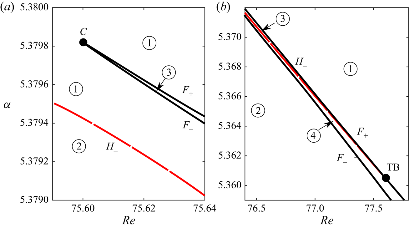
Figure 7. Zooms of figure 5 in the vicinity of the C and TB codimension-two points. Black solid lines denote fold bifurcations  $F_\pm$, long dashed (red) line is used for the Hopf bifurcation line $H_{-}$ and short dashed (red) curve denotes the local change from stable focus to stable node. Numbers correspond to each phase portrait of figure 6(a). (a) Zoom in the region of cusp bifurcation. (b) Zoom in the region of Takens–Bogdanov bifurcation.
3.5.3. Homoclinic bifurcation
As explained in § 3.5, the normal form predicts a homoclinic curve  $H_\infty$ and a homoclinic saddle-node bifurcation along the $F_-$ curve, right from the SNL point, corresponding to the appearance of two steady solutions along a previously existing cycle.
A generic feature of the imminent presence of a homoclinic saddle-node bifurcation is the divergence of the period of the limit cycle on which the saddle node appears. More precisely, the period is expected to scale as  $\propto {1}/{\sqrt {\alpha _{SN}-\alpha }}$ as $\alpha \rightarrow \alpha _{SN}$ (see Gasull, Mañosa & Villadelprat Reference Gasull, Mañosa and Villadelprat2005). To check this prediction, time stepping simulations were conducted for $Re = 170$ and values of $\alpha$ just below the $F_-$ curve. As shown in figure 8 the period of the limit cycle effectively diverges as one approaches the bifurcation following the theoretical behaviour.
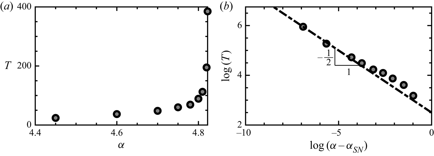
Figure 8. Evolution of the period of the limit cycle as it approaches the homoclinic connection. (a) Linear plot of the period  $T$ as a function of the rotation rate $\alpha$ where $\alpha _{SN}$ is the rotation rate at the saddle node. (b) Logarithm of the period and the distance to the bifurcation point.
Dynamics near the threshold can be perfectly understood in a two-dimensional manifold. Phase portraits of the bifurcation are displayed in figure 9. These phase portraits were computed with an initial guess generated by a small linear perturbation to a steady state in the direction of its corresponding eigenmode. The initial guess is then integrated in time until it reaches its limit set, i.e. a periodic, homoclinic orbit or another steady state. Below the bifurcation threshold (figure 9a) a stable limit cycle exists, represented by a thick solid line. At the bifurcation threshold, a saddle node arises along this cycle, which ceases to exist, giving rise to a homoclinic connection (an approximation of this orbit is delineated by a thick solid line in figure 9b). Beyond the saddle-node bifurcation, the saddle node splits into two fixed points. Hence, three steady states exist, including a stable one (see figure 9c). There exist four stable heteroclinic connections, two between unstable–stable steady states represented by a dashed line in figure 9(c) and other two between saddle–stable steady states denoted by a solid line. This sequence of events is fully consistent to the sequence connecting phase portraits (2), (SNL) and (4) in figure 6.
Figure 9. Phase portrait of the dynamics of the rotating cylinder at  $Re=170$ for three values of the rotation rate $\alpha$. Vertical (horizontal) axis is the lift force $F_y$ (drag force $F_x$) on the cylinder surface, empty dots denote steady-state solutions. (a,b) Limit sets (respectively transients) are depicted by a thick solid line (respectively thin dashed). (c) Heteroclinic connections between unstable–stable (respectively saddle–stable) are depicted by thin solid lines (respectively dashed dotted).
3.6. Generalised Hopf
3.6.1. Normal form analysis
Bautin bifurcation or GH is a codimension-two bifurcation where the equilibrium has purely imaginary eigenvalues  $\lambda _{1,2} = \pm \omega _0$ with $\omega _0 > 0$, and the third-order coefficient of the normal form vanishes. Generalised Hopf bifurcation is thus a degenerate case of the generic Hopf bifurcation, where the cubic normal form is not sufficient to determine the nonlinear stability of the system. To unravel the dynamics near the Bautin bifurcation point consider the normal form
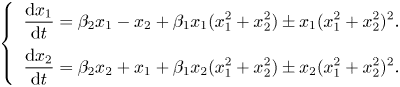 \begin{equation} \left \{\begin{array}{l} \displaystyle\dfrac{\textrm{d} x_1}{\textrm{d} t}= \beta_2 x_1 - x_2 + \beta_1 x_1 ( x_1^2+x_2^2) \pm x_1(x_1^2 + x_2^2)^2. \\ \displaystyle\dfrac{\textrm{d} x_2}{\textrm{d} t}= \beta_2 x_2 + x_1 + \beta_1 x_2 ( x_1^2+x_2^2) \pm x_2(x_1^2 + x_2^2)^2. \\ \end{array} \right.\end{equation}
Three curves are of special interest:
(i) System (3.2) undergoes a supercritical Hopf bifurcation in the half-line
$H_+=\{ (\beta _1,\beta _2) | \beta _2 > 0, \beta _1 = 0 \}$. This curve separates a region containing a stable focus to a region containing an unstable focus plus a stable limit cycle.(ii) System (3.2) undergoes a subcritical Hopf bifurcation in the half-line
$H_-=\{ (\beta _1,\beta _2) | \beta _2 < 0, \beta _1 = 0 \}$. This curve separates a region containing an unstable focus, from one containing a stable focus and two limit cycles (one being stable and the other one being unstable).(iii) System (3.2) undergoes a fold cycle bifurcation on the curve
$F_{LC}=\{ (\beta _1,\beta _2) | \beta _1^2 + 4\beta _2 = 0, \beta _1 < 0 \}$. This curve separates a region containing two limit cycles from one which does not contain any limit cycle (a stable fixed point also exists in both regions).


The most notable feature of this bifurcation is the existence of a bistability region characterised by two stable states (a fixed point and a cycle). Therefore, hysteretic behaviour is expected as one successively crosses curves  $H_-$ and $F_{LC}$. The bistability range is also characterised by the existence of an unstable limit cycle constituting the ‘edge state’ bounding the basins of attraction of the two stable states (figure 10).
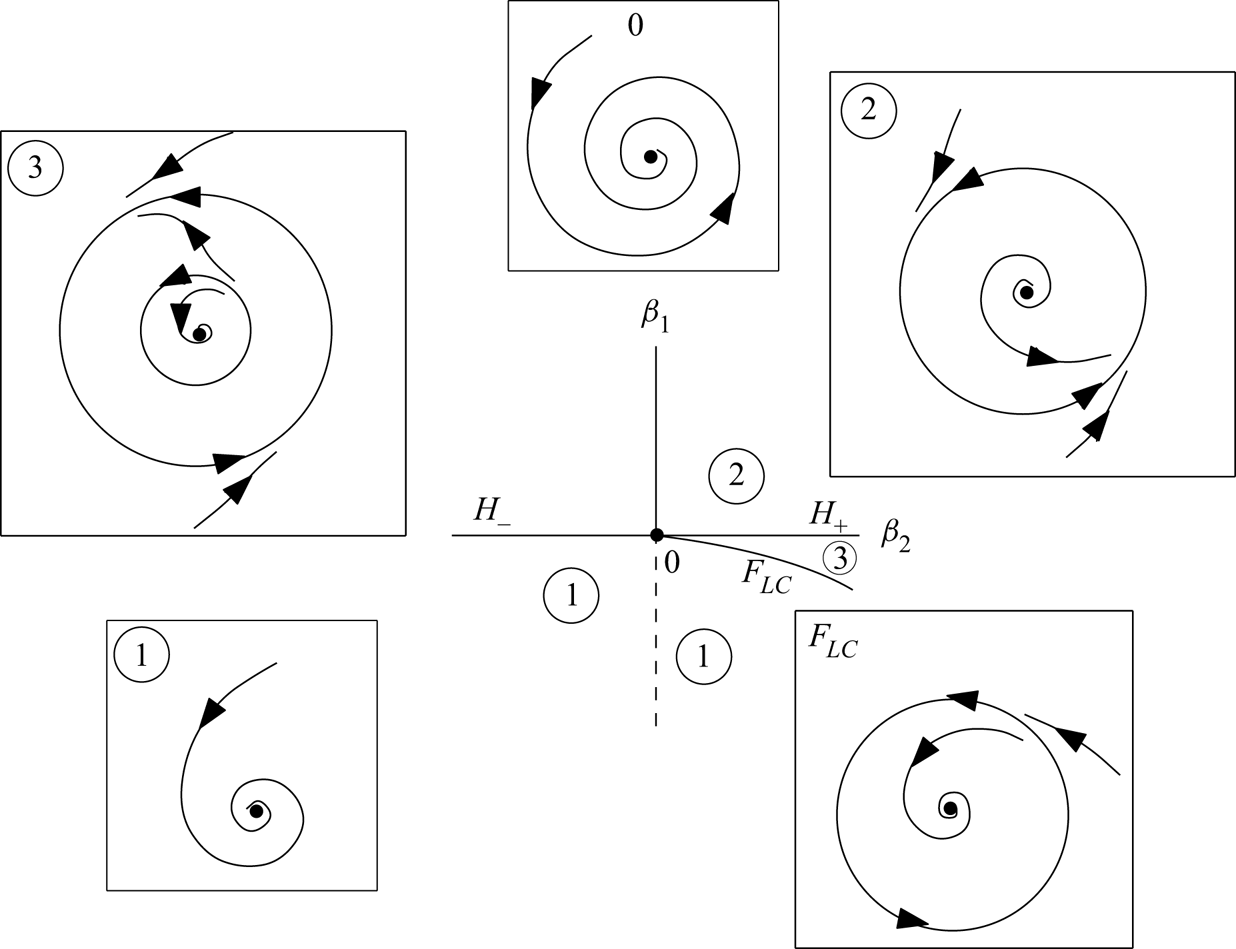
Figure 10. Qualitative bifurcation scenario in the vicinity of the GH bifurcation.
3.6.2. Weakly nonlinear analysis
Unstable limit cycles are not easy to track, since they require stabilisation techniques, such as BoostConv (Citro et al. Reference Citro, Luchini, Giannetti and Auteri2017) or edge-state tracking (Bengana et al. Reference Bengana, Loiseau, Robinet and Tuckerman2019), or the use of continuation techniques, such as harmonic balance (Fabre et al. Reference Fabre, Citro, Sabino, Ferreira, Sierra, Giannetti and Pigou2019). Alternatively, we have performed a multiple-scale analysis up to fifth order (see appendix C). This method was previously used to study thermoacoustic bifurcations in the Rijke tube (Orchini, Rigas & Juniper Reference Orchini, Rigas and Juniper2016), displaying a good match with time stepping simulations with a much lower computational cost. By performing a weakly nonlinear analysis up to fifth order it is possible to determine a complex amplitude equation for the amplitude  $A$ of the critical linear mode $\hat {{\boldsymbol {q}}}$. Here, the critical linear mode is normalised so that its $L^2\mathcal {B}$-norm (see appendix C), i.e. its kinetic energy, is unity, which corresponds to the same normalisation as in Mantič-Lugo, Arratia & Gallaire (Reference Mantič-Lugo, Arratia and Gallaire2014). The governing equation is a Stuart Landau equation, depending on a small parameter $\epsilon ^2 = Re_c(\alpha )^{-1} - Re^{-1}$
 \begin{equation} \frac{\textrm{d} A}{\textrm{d} t} = (\textrm{i} \omega_0 + \epsilon^2 \lambda_0 + \epsilon^4 \lambda_1) A + (\nu_{1,0} + \epsilon^2 \nu_{1,1} ) |A|^2A + \nu_{2,0} |A|^4A. \end{equation}
We remark that (3.3) is equivalent to (3.2) if separating real and imaginary parts. Searching for a solution under the form  $A = |A| \,\textrm {e}^{\textrm {i} \omega t}$, and injecting into (3.3) leads to
 \begin{equation} \left.\begin{array}{c} {}|A| = \sqrt{-\dfrac{\nu_{1,r} }{2\nu_{2,r}} \pm \sqrt{ \dfrac{\nu_{1,r}^2}{4 \nu_{2,r}^2} - \dfrac{\lambda_r}{\nu_{2,r} } }}\\ \omega = \omega_0 + \nu_{1,i}|A| + \nu_{2,i}|A|^2 \end{array}\right\}, \end{equation}
where  $\nu _1 = \nu _{1,0} + \epsilon ^2 \nu _{1,1}$, $\lambda = \epsilon ^2 \lambda _0 + \epsilon ^4 \lambda _1$, $\nu _2 = \nu _{2,0}$ and subscripts $r,i$ denote real and imaginary parts respectively. It turns out that $\nu _{2,r}$ is always negative while $\nu _{1,r}$ changes sign at $(Re,\alpha ) = (Re_{GH},\alpha _{GH})$. One can deduce the following consequences:
(i) If
$Re < Re_{GH}$ (i.e. $\nu _{2r}<0$), (3.4) has a single solution $|A|$ for $\lambda _r >0$ (i.e. $Re>Re_c$) and none for $\lambda _r <0$ (i.e. $Re<Re_c$). In this case, the Hopf bifurcation is supercritical.(ii) If
$Re>Re_{GH}$, (i.e. $\nu _{2r}>0$), (3.4) has a single solution $|A|$ for $\lambda _r >0$ (i.e. $Re>Re_c$), two solutions if $\lambda _c < \lambda _r < 0$ with $\lambda _c = {\nu _{1,r}^2}/{4 \nu _{2,r}}$ and no solution if $\lambda _r <\lambda _c$. In this case, the Hopf bifurcation is subcritical. The condition $\lambda _r = \lambda _c$ defines a curve in the $(Re,\alpha )$ plane which corresponds to the fold cycle bifurcation associated with the emergence of the two limit cycles.


Figure 11 represents the amplitude and frequency of the limit cycles predicted by (3.4) for three values of  $Re$. According to these results, the fold curve is predicted to be very close to the Hopf curve, i.e. within a few tenths of $Re$ up to $Re=250$. This behaviour allows us to clarify the transition occurring at the GH point in figure 6. For $Re<Re_{GH}$, when increasing $Re$ for fixed $\alpha$ (or increasing $\alpha$ with fixed $Re$), the transition occurs via a supercritical Hopf bifurcation. On the other hand, for $Re>Re_{GH}$, the transition is predicted to be subcritical, involving the existence of a band where both steady state and Mode II coexist. Note that the width of the bistability band predicted by the weakly nonlinear analysis is very narrow, and could thus be difficult to evidence using direct numerical simulations.
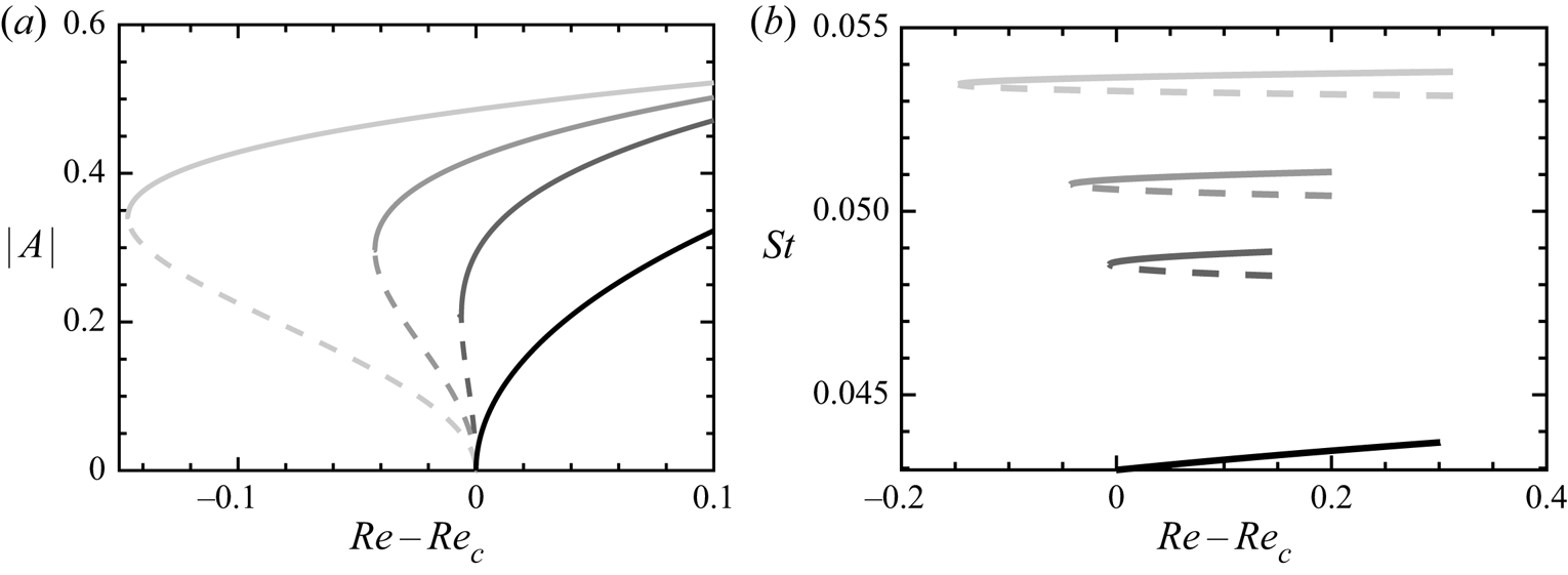
Figure 11. (a) Amplitudes of stable (solid line) and unstable (dashed line) limit cycles for four  $Re_c=100;170;200;250$, where $Re_c$ denotes the Reynolds number at the Hopf bifurcation. Grey scale: darker curves designate quantities associated with a lower $Re$, i.e. black curve $Re=100$ and light grey $Re = 250$. (b) Strouhal number of limit cycles.
4. Conclusion and discussion
The present study allowed us to clarify the bifurcation scenario in the two-dimensional flow past a rotating cylinder, especially concerning the range of parameters corresponding to the onset of the ‘Mode II’ unsteady vortex shedding mode. Using steady-state calculation involving arclength continuation and linear stability analysis, we have been able to draw all bifurcation curves existing in the range of parameters corresponding to  $Re <200$ and $\alpha <5$. Three codimension-two bifurcations have been identified along the border of the range of existence of this mode, namely a Takens–Bogdanov, a cusp and a generalised Hopf. The first two are located in close vicinity, in such a way that the whole dynamics can be understood using the normal form of the codimension-three bifurcation (for a generalised Takens–Bogdanov bifurcation). The analysis also allowed us to identify three ranges of parameters characterised by bistability, two of them located in the vicinity of the Takens–Bogdanov and cusp points, the third one emanating from the generalised Hopf point. Time stepping simulations and a weakly nonlinear analysis have confirmed these findings, and have also allowed us to characterise the homoclinic and heteroclinic orbits connecting the fixed points, in full accordance with the predictions of the normal form theory.
The most surprising result of the study is the existence of an almost perfect codimension-three bifurcation in a problem characterised by only two control parameters. Such a feature suggests that the problem could be quite sensible to any small perturbations in a way such that small perturbations could completely change the scenario. We have checked that the scenario is robust with respect to numerical discretisation issues (see appendix D). The dependency with respect to additional physical parameters is more interesting. The effect of compressibility is an interesting question which we expect to investigate in future studies. Preliminary results have shown that for a Mach number of order 0.1, the dynamics in the region of the near-codimension-three point is effectively greatly modified. Other additional parameters, such as for instance shear or confinement, could be added. Finally, one may question the relevance of the present findings for three-dimensional flows. A short review of three-dimensional stability properties of the rotating cylinder flow is given in appendix E. The discussion confirms that the most important results of the present study occur in range of parameters where no three-dimensional instabilities are present.
Declaration of interests
The authors report no conflict of interest.
Appendix A. Pseudo arc-length continuation
Arc-length continuation is a standard technique in dynamical systems theory. It allows for the continuation of a given solution branch through a turning or fold point. At the turning point the Jacobian of the system is singular; therefore, any iterative method based on the Jacobian is doomed to failure. To prevent the stall in the convergence of the Newton's method, an extra condition needs to be added to the system of equations. In the current study we have chosen a pseudo arc-length methodology, which is based in a predictor–corrector strategy. The extended system adds an extra equation which ensures the tangency to the branch of the solution. For that purpose, a parameter is chosen, here either  $Re$ or $\alpha$, and a monitor of the variation, either the horizontal force acting on the cylinder surface $F_x$ or the vertical force $F_y$. The parameter and the monitor are parametrised by the length of the branch, here indicated by the parameter $s$. The current solution is varied by a given step ${\rm \Delta} s$ tangent to the solution branch and later corrected by a orthogonal correction. Let us denote by the subscript $j$ the arc-length iteration and by the superscript $n$ the Newton iteration of the corrector step, where $N$ is used to denote the last step. In the description below, let us consider without loss of generality we have fixed the parameter $\alpha$ and the monitor $F_x$.
A.1. Predictor
The predictor step consists in the determination of a initial guess  $\alpha ^0_j$ for the iteration $j$ of the arc length. The initial guess is determined from a tangent extrapolation of the solution branch.
 \begin{gather} \alpha^0_j = \alpha^N_{j-1} + \frac{\textrm{d} \alpha^N_{j-\textrm{1}}}{ds} {\rm \Delta} s, \end{gather}
 \begin{gather}{\boldsymbol{q}}^0_j = {\boldsymbol{q}}^N_{j-1} + \frac{\textrm{d} {\boldsymbol{q}}^N_{j-1}}{\textrm{d}s} {\rm \Delta} s \implies F_x({\boldsymbol{q}}^0_j) = F_x({\boldsymbol{q}}^N_{j-1}) + \frac{\textrm{d} F_x({\boldsymbol{q}}^N_{j-1})}{\textrm{d}s} {\rm \Delta} s. \end{gather}
 In (A 1),  ${\textrm {d} \alpha ^N_{j-1}}/{\textrm {d}s}$ is the slope of the tangent in the $\alpha$ direction and ${\textrm {d}{\boldsymbol {q}}^N_{j-1}}/{\textrm {d}s}$ in the direction of the vector field. The tangent is computed from the differentiation of the stationary Navier–Stokes equations (2.1)
 \begin{equation} \frac{\textrm{d} {\boldsymbol{q}}^N_{j-1}}{\textrm{d}s} = - \left[\frac{\partial{NS}_{{\boldsymbol{q}}^N_{j-1}}}{\partial {\boldsymbol{q}}} \right]^{-1}\frac{\partial{NS}_{{\boldsymbol{q}}^N_{j-1}}}{\partial \alpha}, \end{equation}
where we have used the notation  ${NS}_{\boldsymbol {q}^N_{j-1}} = 0$ to denote the steady incompressible Navier–Stokes equation whose solution is $\boldsymbol {q}^N_{j-1}$. The tangent is completed with a normalisation condition in the arc length
 \begin{equation} \left\lVert\frac{\textrm{d} F_x(\boldsymbol{q}^N_{j-1})}{\textrm{d}s}\right\rVert_2^2 + \left\lVert\frac{\textrm{d} \alpha^N_{j-1}}{\textrm{d}s}\right\rVert_2^2 = 1. \end{equation}
A.2. Corrector
This step consists in an orthogonal correction of the tangent guess. To do so one needs to solve the following system of equations
 \begin{equation} \begin{bmatrix} \frac{\partial{NS}_{\boldsymbol{q}^n_{j}}}{\partial \boldsymbol{q}} & \frac{\partial{NS}_{\boldsymbol{q}^n_{j}}}{\partial \alpha} \\ \frac{\textrm{d} F_x(\boldsymbol{q}^n_{j1})}{\textrm{d}s} F_x(\cdot) & \frac{\textrm{d} \alpha^n_{j}}{\textrm{d}s} \end{bmatrix} \begin{bmatrix} {\rm \Delta} \boldsymbol{q}_{j}^{n+1} \\ {\rm \Delta} \alpha_{j}^{n+1} \end{bmatrix} = \begin{bmatrix} -NS({\boldsymbol{u}}) \\ {\rm \Delta} s - \frac{\textrm{d}{F_x}}{\textrm{d} s} F_x(\boldsymbol{q}^n_{j} - \boldsymbol{q}^N_{j-1}) - \frac{\textrm{d}{\alpha}}{\textrm{d} s}(\alpha^n_{j} - \alpha^N_{j-1}) \end{bmatrix}, \end{equation}
where the last equation of (A 4) comes from the differentiation of the normalisation condition (A 3) and considering that  ${\rm \Delta} \alpha _j = {\rm \Delta} \alpha _j^{n+1} + \alpha _j^n - \alpha _{j-1}^N = \alpha _j^{N} - \alpha _{j-1}^N$ (similarly on $\boldsymbol {q}$).
Appendix B. Weakly nonlinear analysis to determine the normal form of the saddle-node bifurcation
Saddle-node bifurcation and homoclinic saddle-node bifurcation are locally characterised by the normal form of the saddle-node bifurcation (see Kuznetsov Reference Kuznetsov2013). In the generic case, when  $a_2(Re,\alpha ) \neq 0$ and $a_0(Re,\alpha ) \neq 0$ the central manifold is unravelled by its second-order normal form
 \begin{equation} \frac{\textrm{d} x_1}{\textrm{d}t} = a_0(Re,\alpha) + a_2(Re,\alpha) x_1^2 + O(x_1^3). \end{equation}
Coefficients  $a_2(Re,\alpha ) \neq 0$ and $a_0(Re,\alpha ) \neq 0$ can be obtained with aid of weakly nonlinear analysis. Let us consider the following transformations:
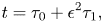 \begin{gather} t = \tau_0 + \epsilon^2 \tau_1, \end{gather}
 \begin{gather}\frac{\textrm{d}}{\textrm{d}t} = \frac{\textrm{d}}{\textrm{d}\tau_0} + \epsilon^2 \frac{\textrm{d}}{\textrm{d}\tau_1}, \end{gather}
 \begin{gather}\boldsymbol{Q} = \boldsymbol{Q}_b + \epsilon {\hat{\boldsymbol{q}}} + \epsilon^2 \boldsymbol{q}_2, \end{gather}
where  $\epsilon ^2 = ({1}/{Re_c}) - ({1}/{Re})$. The system at order $\epsilon ^0$ is the incompressible Navier–Stokes system that provides the base flow. The system at order $\epsilon ^1$ is identical to the linearised Navier–Stokes problem (2.3). At order $\epsilon ^2$ secular term appears and solvability condition must be imposed
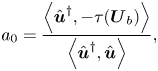 \begin{gather} a_0 = \frac{ \left\langle {\hat{\boldsymbol{u}}}^{\dagger}, -\tau(\boldsymbol{U}_b) \right\rangle} {\left\langle \hat{\boldsymbol{u}}^{\dagger},\hat{\boldsymbol{u}} \right\rangle}, \end{gather}
 \begin{gather}a_2 = \frac{ \left\langle {\hat{\boldsymbol{u}}}^{\dagger}, -\hat{\boldsymbol{u}} \boldsymbol{\nabla} \hat{\boldsymbol{u}} \right\rangle} { \left\langle \hat{\boldsymbol{u}}^{\dagger},\hat{\boldsymbol{u}} \right\rangle}. \end{gather}
Here,  $\hat {\boldsymbol {u}}^\dagger$ denotes the adjoint or left eigenvector of linearised Navier–Stokes equations associated with the null eigenvalue.
Appendix C. WNL to determine the normal form of the Hopf bifurcation degeneracy
Weakly nonlinear analysis has been used extensively in the case of Hopf bifurcations to unravel the frequency of the limit cycle near the bifurcation threshold (see Gallaire et al. Reference Gallaire, Boujo, Mantic-Lugo, Arratia, Thiria and Meliga2016) and to determine the validity of stability analysis on the mean flow (see Sipp & Lebedev Reference Sipp and Lebedev2007). In this article WNL analysis is used to determine the existence of a generalised Hopf bifurcation (see § 3.6). The starting point of the weakly nonlinear method is the decomposition of the flow field into multiple scales
 \begin{align} \boldsymbol{Q} &= \boldsymbol{Q}_{\boldsymbol{b}} + \epsilon \left[A_{wnl} \hat{\boldsymbol{q}} \,\textrm{e}^{\textrm{i}\omega_0 t} + \textrm{c.c.}\right] \nonumber\\ &\quad + \epsilon^2 \left [\boldsymbol{q}_{2,0} + |A_{wnl}| \boldsymbol{q}^{|A_{wnl}|}_{2,0} + (A^2_{wnl}\boldsymbol{q}_{2,2}\, \textrm{e}^{2\textrm{i}\omega_0 t} + \textrm{c.c.} ) \right] \nonumber\\ &\quad + \epsilon^3\left[ A_{wnl}\,\textrm{e}^{\textrm{i}\omega_0 t} \left(\boldsymbol{q}_{3,1} + |A_{wnl}|^2\boldsymbol{q}_{3,1}^{|A_{wnl}|^2} + |A_{wnl}|^2\boldsymbol{q}_{3,1}^{A_{wnl} \bar{A}_{wnl}} \right) + A_{wnl}^3 \,\textrm{e}^{3\textrm{i}\omega_0t} \boldsymbol{q}_{3,3} + \textrm{c.c.} \right] \nonumber\\ &\quad + \epsilon^4 \left[\boldsymbol{q}_{4,0} + |A_{wnl}|^2 \boldsymbol{q}^{|A_{wnl}|^2}_{4,0} + |A_{wnl}|^4 \boldsymbol{q}^{|A_{wnl}|^4}_{4,0} \right. \nonumber\\ &\quad \left. + A_{wnl}^2 \,\textrm{e}^{2\textrm{i} \omega_0 t} \left( \boldsymbol{q}_{4,2} + |A_{wnl}|^2\boldsymbol{q}^{|A_{wnl}|^2}_{4,2} \right) + A_{wnl}^4 \,\textrm{e}^{4\textrm{i} \omega_0 t} \boldsymbol{q}_{4,4} + \textrm{c.c.} \right] + O(\epsilon^5), \end{align}
where the complex amplitude  $A_{wnl}$ depends upon a slow time scale $\tau = \epsilon ^2 t$. The choice of the parameter $\epsilon$ is the same as in Fabre et al. (Reference Fabre, Citro, Sabino, Ferreira, Sierra, Giannetti and Pigou2019), $\epsilon ^2 = {1}/{Re_c(\alpha )}-{1}/{Re}$, where the critical Reynolds $Re_c(\alpha )$ is a function of the rotation rate $\alpha$. When the ansatz (C 1) is substituted into the Navier–Stokes equations, at orders $O(\epsilon ^3)$ and $O(\epsilon ^5)$ solvability conditions need to be imposed due to the presence of secular terms which lead to a Stuart–Landau equation depending upon the slow time scale $\tau$
 \begin{equation} \frac{\partial A_{wnl}}{\partial \tau} = (\lambda_0 + \epsilon^2 \lambda_1) A_{wnl} + (\nu_{1,0} + \epsilon^2 \nu_{1,1} ) |A_{wnl}|^2A_{wnl} + \epsilon^2 \nu_{2,0} |A_{wnl}|^4A_{wnl}. \end{equation}
If we take into account the definition of the slow time scale  $\tau = \epsilon ^2 t$, the fact that up to leading order $O(\epsilon )$ we have ${\textrm {d} A_{wnl}}/{\textrm {d}t} = \textrm {i} \omega _0 \epsilon A_{wnl}$ and we define a new amplitude which depends on $\epsilon$ as $A = \epsilon A_{wnl}$ we can rewrite (C 2) as
 \begin{equation} \frac{\textrm{d} A}{\textrm{d} t} = (\textrm{i} \omega_0 + \epsilon^2 \lambda_0 + \epsilon^4 \lambda_1) A + (\nu_{1,0} + \epsilon^2 \nu_{1,1} ) |A|^2A + \nu_{2,0} |A|^4A. \end{equation}
In the following we consider that the eigenmode  $\hat {\boldsymbol {q}}$ and its adjoint $\hat {\boldsymbol {q}}^{\dagger}$ have been normalised so that $||\hat {\boldsymbol {q}}||^2_\mathcal {B} = \left \langle \hat {\boldsymbol {q}}, \mathcal {B} \hat {\boldsymbol {q}} \right \rangle = \left \langle \hat {\boldsymbol {u}}, \hat {{\boldsymbol {u}}} \right \rangle = 1$ and $\left \langle \hat {\boldsymbol {q}}^{\dagger} , \mathcal {B} \hat {\boldsymbol {q}} \right \rangle = \left \langle \hat {{\boldsymbol {u}}}^{\dagger} , \hat {{\boldsymbol {u}}} \right \rangle = 1$. This normalisation is the same as that one used in the self-consistent methodology (see Mantič-Lugo et al. Reference Mantič-Lugo, Arratia and Gallaire2014): with this choice, $A$ is a real constant representing the amplitude of the linear mode with respect to its $L^2$ norm. In the following we will use the notation $\mathcal {LNS}_{\textrm {i} \omega } \boldsymbol {q} = \textrm {i} \omega {\mathcal {B}} \boldsymbol {q} - \mathcal {LNS} \boldsymbol {q}$ to denote the application of the linearised operator at a specific frequency $\omega$.
The ansatz (C 1) is substituted into the incompressible Navier–Stokes equations (2.1):
(i) Order
$O(\epsilon ^0)$ leads to the steady-state Navier–Stokes equations (2.1).(ii) Order
$O(\epsilon ^1)$ leads to the linearised Navier–Stokes equations (2.3).(iii) Order
$O(\epsilon ^2)$ contains three terms, which are computed as the solution of three linear systems:
(C 4a)\begin{gather} \mathcal{LNS}_{0} \boldsymbol{q}_{2,0} = - 2 \boldsymbol{\nabla} \boldsymbol{\cdot} (d(\boldsymbol{U}_b)), \end{gather}(C 4b)\begin{gather}\mathcal{LNS}_{0} {\boldsymbol{u}}_{2,0}^{|A_{wnl}|} = - \hat{\boldsymbol{q}}\boldsymbol{\cdot} \boldsymbol{\nabla} \bar{\hat{{\boldsymbol{u}}}} + \bar{\hat{{\boldsymbol{u}}}}\boldsymbol{\cdot} \boldsymbol{\nabla} \hat{\boldsymbol{q}}, \end{gather}(C 4c)\begin{gather}\mathcal{LNS}_{2 \textrm{i} \omega_0} {\boldsymbol{u}}_{2,2} = - \hat{{\boldsymbol{u}}}\boldsymbol{\cdot} \boldsymbol{\nabla} \hat{{\boldsymbol{u}}}. \end{gather}(iv) At order
$O(\epsilon ^3)$ there are degenerate terms, i.e. terms corresponding to the frequency $\textrm {i} \omega _0$. The operator $\mathcal {LNS}_{\textrm {i} \omega _0}$ is not injective ($\hat {\boldsymbol {q}}$ belongs to its kernel) and it is not surjective because $\hat {\boldsymbol {q}}^{\dagger}$ belongs to the kernel of its adjoint and the operator is Fredholm in $L^2$. Therefore we need to impose solvability conditions in order to obtain terms $\boldsymbol {q}_{3,1}$, $\boldsymbol {q}_{3,1}^{|A_{wnl}|^2}$ and $\boldsymbol {q}_{3,1}^{A_{wnl}\bar {A}_{wnl}}$. Solvability conditions at $O(\epsilon ^3)$ correspond to
(C 5)\begin{gather} \mu_1 = -\frac{ \left\langle {\hat{\boldsymbol{u}}}^{\dagger}, \hat{\boldsymbol{u}}\boldsymbol{\cdot} \boldsymbol{\nabla} {\boldsymbol{u}}_{2,0}^{|A_{wnl}|} + {\boldsymbol{u}}_{2,0}^{|A_{wnl}|}\boldsymbol{\cdot} \boldsymbol{\nabla} \hat{\boldsymbol{u}} \right\rangle} { \left\langle \hat{\boldsymbol{u}}^{\dagger},\hat{\boldsymbol{u}} \right\rangle}, \end{gather}(C 6)\begin{gather}\mu_2 = -\frac{ \left\langle {\hat{\boldsymbol{u}}}^{\dagger}, \bar{\hat{\boldsymbol{u}}} \boldsymbol{\cdot} \boldsymbol{\nabla} {\boldsymbol{u}}_{2,2} + {\boldsymbol{u}}_{2,2} \boldsymbol{\cdot} \boldsymbol{\nabla} \bar{\hat{\boldsymbol{u}}} \right\rangle} {\left\langle \hat{\boldsymbol{u}}^{\dagger},\hat{\boldsymbol{u}} \right\rangle}, \end{gather}(C 7)where\begin{gather}\lambda_0 =- \frac{ \left\langle {\hat{\boldsymbol{u}}}^{\dagger}, \hat{\boldsymbol{u}}\boldsymbol{\cdot} \boldsymbol{\nabla} {\boldsymbol{u}}_{2,0} + {\boldsymbol{u}}_{2,0} \boldsymbol{\cdot} \boldsymbol{\nabla} \hat{\boldsymbol{u}} + 2 \boldsymbol{\nabla} \boldsymbol{\cdot}(d(\hat{\boldsymbol{u}})) \right\rangle} { \left\langle \hat{\boldsymbol{u}}^{\dagger},\hat{\boldsymbol{u}} \right\rangle}, \end{gather}$\mu _1 + \mu _2 = \nu _{1,0}$. Additionally, given the fact that $L^2$ is a Hilbert space and the operator is Fredholm, the space can be decomposed into a direct sum of the range of the operator $\mathcal {LNS}_{\textrm {i} \omega _0}$ and the kernel of its adjoint. This implies that secular terms are determined up to a constant in the direction of the eigenmode $\hat {\boldsymbol {q}}$, i.e. $\boldsymbol {q}_{3,1} \rightarrow \boldsymbol {q}_{3,1} + \delta _0 \hat {\boldsymbol {q}}$, $\delta _0 \in \mathbb {R}$. This degree of freedom is fixed by considering $\delta _0 = 0$, i.e. each secular term is orthogonal to the linear adjoint mode $\hat {\boldsymbol {q}}^{\dagger}$ in the norm $\mathcal {B}$, i.e. $\left \langle \hat {\boldsymbol {q}}^{\dagger} , \mathcal {B} \boldsymbol {q}_{3,1} \right \rangle = 0$. This choice for the extra degree of freedom has been also used in Carini, Auteri & Giannetti (Reference Carini, Auteri and Giannetti2015). This leads to
(C 8)and similarly for pairs\begin{equation} \begin{pmatrix} \mathcal{LNS}_{\textrm{i}\omega_0} & -\mathcal{B}\hat{\boldsymbol{q}} \\ \hat{\boldsymbol{q}}^{{\dagger} H} \mathcal{B} & 0 \end{pmatrix} \begin{pmatrix} \boldsymbol{q}_{3,1} \\ \lambda_0 \end{pmatrix} = \begin{pmatrix} \boldsymbol{F}_{3,1} \\ 0 \end{pmatrix} \end{equation}$(\boldsymbol {q}_{3,1}^{|A_{wnl}|^2},\mu _1)$ and $(\boldsymbol {q}_{3,1}^{A_{wnl}\bar {A}_{wnl}},\mu _2$ replacing ${\boldsymbol {F}}_{3,1}$ by ${\boldsymbol {F}}_{3,1}^{|A_{wnl}|^2}$ and ${\boldsymbol {F}}_{3,1}^{A_{wnl}\bar {A}_{wnl}}$ respectively. Please note that
(C 9)The other non-resonant term is solved as usually,\begin{equation} \left.\begin{gathered} {\boldsymbol{F}}_{3,1} = -\hat{\boldsymbol{u}}\boldsymbol{\cdot} \boldsymbol{\nabla} {\boldsymbol{u}}_{2,0} - {\boldsymbol{u}}_{2,0}\boldsymbol{\cdot} \boldsymbol{\nabla} \hat{\boldsymbol{u}} - 2 \boldsymbol{\nabla} \boldsymbol{\cdot} (d(\hat{\boldsymbol{u}}))\\ {\boldsymbol{F}}_{3,1}^{|A_{wnl}|^2} = -\hat{\boldsymbol{u}} \boldsymbol{\cdot}\boldsymbol{\nabla} {\boldsymbol{u}}_{2,0}^{|A_{wnl}|} - {\boldsymbol{u}}_{2,0}^{|A_{wnl}|} \boldsymbol{\cdot} \boldsymbol{\nabla} \hat{\boldsymbol{u}}\\ {\boldsymbol{F}}_{3,1}^{A_{wnl}\bar{A}_{wnl}} = - \bar{\hat{\boldsymbol{u}}}\boldsymbol{\cdot} \boldsymbol{\nabla} {\boldsymbol{u}}_{2,2} - {\boldsymbol{u}}_{2,2} \boldsymbol{\cdot} \boldsymbol{\nabla} \bar{\hat{\boldsymbol{u}}} \end{gathered}\right\}. \end{equation}(C 10)\begin{equation} \mathcal{LNS}_{3 \textrm{i} \omega_0} \boldsymbol{q}_{3,3} = {\boldsymbol{F}}_{3,3} = - \hat{\boldsymbol{u}}\boldsymbol{\cdot} \boldsymbol{\nabla} {\boldsymbol{u}}_{2,2} - {\boldsymbol{u}}_{2,2}\boldsymbol{\cdot} \boldsymbol{\nabla} \hat{\boldsymbol{u}}. \end{equation}(v) At order
$O(\epsilon ^4)$ we find six terms which are solved by the resolution of the following linear systems
(C 11)where the right-hand side terms are\begin{equation} \left.\begin{aligned} \mathcal{LNS}_{0} \boldsymbol{q}_{4,0} = {\boldsymbol{F}}_{4,0} \\ \mathcal{LNS}_{0} \boldsymbol{q}^{|A_{wnl}|^2}_{4,0} = {\boldsymbol{F}}^{|A_{wnl}|^2}_{4,0} \\ \mathcal{LNS}_{0} \boldsymbol{q}^{|A_{wnl}|^4}_{4,0} = {\boldsymbol{F}}^{|A_{wnl}|^4}_{4,0} \\ \mathcal{LNS}_{2 \textrm{i} \omega_0} \boldsymbol{q}_{4,2} = {\boldsymbol{F}}_{4,2} \\ \mathcal{LNS}_{2 \textrm{i} \omega_0} \boldsymbol{q}^{|A_{wnl}|^2}_{4,2} = {\boldsymbol{F}}^{|A_{wnl}|^2}_{4,2} \\ \mathcal{LNS}_{4 \textrm{i} \omega_0} \boldsymbol{q}_{4,4} = {\boldsymbol{F}}_{4,4} \end{aligned}\right\}, \end{equation}(C 12)\begin{align} \boldsymbol{F}_{4,0} &= -\boldsymbol{u}_{2,0}\boldsymbol{\cdot} \boldsymbol{\nabla} \boldsymbol{u}_{2,0} - 2 \boldsymbol{\nabla} \boldsymbol{\cdot} d(\boldsymbol{u}_{2,0}),\\ \boldsymbol{F}^{|A_{wnl}|^2}_{4,0} &= -\boldsymbol{u}_{3,1} \boldsymbol{\cdot} \boldsymbol{\nabla} \bar{\hat{\boldsymbol{u}}} - \bar{\hat{\boldsymbol{u}}} \boldsymbol{\cdot} \boldsymbol{\nabla} \boldsymbol{u}_{3,1} - \bar{\boldsymbol{u}}_{3,1} \boldsymbol{\cdot} \boldsymbol{\nabla} \hat{\boldsymbol{u}} - \hat{\boldsymbol{u}} \boldsymbol{\cdot} \boldsymbol{\nabla} \bar{\boldsymbol{u}}_{3,1} \nonumber\\ &\quad -\boldsymbol{u}_{2,0}\boldsymbol{\cdot} \boldsymbol{\nabla} \boldsymbol{u}^{|A_{wnl}|^2}_{2,0} \boldsymbol{u}^{|A_{wnl}|^2}_{2,0} \boldsymbol{\cdot} \boldsymbol{\nabla} \boldsymbol{u}_{2,0},\\ \boldsymbol{F}^{|A_{wnl}|^4}_{4,0} &= -\boldsymbol{u}_{2,2} \boldsymbol{\cdot} \boldsymbol{\nabla} \bar{\boldsymbol{u}}_{2,2} - \bar{\boldsymbol{u}}_{2,2} \boldsymbol{\cdot} \boldsymbol{\nabla} \boldsymbol{u}_{2,2} - \boldsymbol{u}^{|A_{wnl}|^2}_{2,0}\boldsymbol{\cdot} \boldsymbol{\nabla} - \boldsymbol{u}^{|A_{wnl}|^2}_{2,0} \nonumber\\ &\quad - \boldsymbol{u}_{3,1}^{|A_{wnl}|^2}\boldsymbol{\cdot} \boldsymbol{\nabla} \bar{\hat{\boldsymbol{u}}} - \bar{\hat{\boldsymbol{u}}} \boldsymbol{\cdot} \boldsymbol{\nabla} \boldsymbol{u}_{3,1}^{|A_{wnl}|^2} - \bar{\boldsymbol{u}}_{3,1}^{|A_{wnl}|^2}\boldsymbol{\cdot} \boldsymbol{\nabla} \hat{\boldsymbol{u}} - \hat{\boldsymbol{u}}\boldsymbol{\cdot} \boldsymbol{\nabla}\bar{\boldsymbol{u}}_{3,1}^{|A_{ wnl}|^2} \nonumber\\ &\quad - \boldsymbol{u}_{3,1}^{A_{wnl} \bar{A}_{wnl}}\boldsymbol{\cdot} \boldsymbol{\nabla} \bar{\hat{\boldsymbol{u}}} - \bar{\hat{\boldsymbol{u}}}\boldsymbol{\cdot} \boldsymbol{\nabla} \boldsymbol{u}_{3,1}^{A_{wnl} \bar{A}_{wnl}} - \bar{\boldsymbol{u}}_{3,1}^{A_{wnl} \bar{A}_{wnl}}\boldsymbol{\cdot} \boldsymbol{\nabla} \hat{\boldsymbol{u}} - \hat{\boldsymbol{u}}\boldsymbol{\cdot} \boldsymbol{\nabla}\bar{\boldsymbol{u}}_{3,1}^{ A_{wnl} \bar{A}_{wnl}},\\ \boldsymbol{F}_{4,2} &= -\boldsymbol{u}_{2,0}^{|A|^2_{wnl}}\boldsymbol{\cdot} \boldsymbol{\nabla} \boldsymbol{u}_{2,0} - \boldsymbol{u}_{2,0} \boldsymbol{\cdot}\boldsymbol{\nabla} \boldsymbol{u}^{|A|^2_{wnl}}_{2,0} - \boldsymbol{u}_{3,1} \boldsymbol{\cdot} \boldsymbol{\nabla} \hat{\boldsymbol{u}} - \hat{\boldsymbol{u}} \boldsymbol{\cdot} \boldsymbol{\nabla} \boldsymbol{u}_{3,1} \nonumber\\ &\quad- 2 \boldsymbol{\nabla} \boldsymbol{\cdot} d(\boldsymbol{u}_{2,2}),\\ \boldsymbol{F}^{|A_{wnl}|^2}_{4,2} &= - \boldsymbol{u}_{2,0} \boldsymbol{\cdot} \boldsymbol{\nabla} \boldsymbol{u}_{2,2} - \boldsymbol{u}_{2,2} \boldsymbol{\cdot} \boldsymbol{\nabla} \boldsymbol{u}_{2,0} - \boldsymbol{u}_{3,1}^{|A_{wnl}|^2}\boldsymbol{\cdot} \boldsymbol{\nabla} \hat{\boldsymbol{u}} - \hat{\boldsymbol{u}}\boldsymbol{\cdot} \boldsymbol{\nabla}\boldsymbol{u}_{3,1}^{|A_{wnl}|^2} \nonumber\\ &\quad - \boldsymbol{u}_{3,1}^{A_{wnl} \bar{A}_{wnl}}\boldsymbol{\cdot}\boldsymbol{\nabla} \hat{\boldsymbol{u}} - \hat{\boldsymbol{u}}\boldsymbol{\cdot} \boldsymbol{\nabla}\boldsymbol{u}_{3,1}^{A_{wnl} \bar{A}_{wnl}} - \boldsymbol{u}_{3,3}\boldsymbol{\cdot} \boldsymbol{\nabla}\bar{\hat{\boldsymbol{u}}} - \bar{\hat{\boldsymbol{u}}} \boldsymbol{\cdot} \boldsymbol{\nabla} \boldsymbol{u}_{3,3}, \end{align}(C 13)\begin{align} \boldsymbol{F}_{4,4} &= -\boldsymbol{u}_{2,2} \boldsymbol{\cdot} \boldsymbol{\nabla} \boldsymbol{u}_{2,2} - \boldsymbol{u}_{3,3} \boldsymbol{\cdot} \boldsymbol{\nabla} \hat{\boldsymbol{u}} - \hat{\boldsymbol{u}} \boldsymbol{\cdot} \boldsymbol{\nabla} \boldsymbol{u}_{3,3}. \end{align}(vi) At order
$O(\epsilon ^5)$ we find three degenerate terms proportional to $A_{wnl}$, $A_{wnl}|A_{wnl}|^2$ and $A_{wnl}|A_{wnl}|^4$. As for the case of the third-order solvability conditions, they lead to the computation of coefficients $\lambda _1$, $\nu _{1,1}$ and $\nu _{2,0}$
(C 14)where\begin{equation} \left.\begin{aligned} & \lambda_1 = \left\langle \hat{\boldsymbol{u}}^{\dagger} , \boldsymbol{F}_{5,1} \right\rangle \\ & \nu_{1,1} = \left\langle \hat{\boldsymbol{u}}^{\dagger} , \boldsymbol{F}_{5,1}^{A_{wnl}|A_{wnl}|^2} \right\rangle \\ & \nu_{2,0}= \left\langle \hat{\boldsymbol{u}}^{\dagger} , \boldsymbol{F}_{5,1}^{A_{wnl}|A_{wnl}|^4} \right\rangle \end{aligned}\right\}, \end{equation}$\boldsymbol {F}_{5,1}$, $\boldsymbol {F}_{5,1}^{|A_{wnl}|^2}$ and $\boldsymbol {F}_{5,1}^{|A_{wnl}|^4}$ are defined as follows:
(C 15)\begin{align} \boldsymbol{F}_{5,1} &= -\boldsymbol{u}_{2,0} \boldsymbol{\cdot} \boldsymbol{\nabla} \boldsymbol{u}_{3,1} - \boldsymbol{u}_{2,0} \boldsymbol{\cdot} \boldsymbol{\nabla} \boldsymbol{u}_{3,1} - \boldsymbol{u}_{4,0} \boldsymbol{\cdot} \boldsymbol{\nabla} \hat{\boldsymbol{u}} - \hat{\boldsymbol{u}} \boldsymbol{\cdot} \boldsymbol{\nabla} \boldsymbol{u}_{4,0} \nonumber\\ &\quad - 2 \boldsymbol{\nabla} \boldsymbol{\cdot} d(\boldsymbol{u}_{3,1}),\\ \boldsymbol{F}_{5,1}^{A_{wnl}|A_{wnl}|^2} &= -\boldsymbol{u}_{2,0} \boldsymbol{\cdot} \boldsymbol{\nabla} \boldsymbol{u}_{3,0}^{|A_{wnl}|^2} - \boldsymbol{u}_{3,0}^{|A_{wnl}|^2} \boldsymbol{\cdot} \boldsymbol{\nabla} \boldsymbol{u}_{2,0} \nonumber\\ &\quad - \boldsymbol{u}_{2,0} \boldsymbol{\cdot} \boldsymbol{\nabla} \boldsymbol{u}_{3,0}^{A_{wnl}\bar{A}_{wnl}} - \boldsymbol{u}_{3,0}^{A_{wnl}\bar{A}_{wnl}} \boldsymbol{\cdot} \boldsymbol{\nabla} \boldsymbol{u}_{2,0} \nonumber\\ &\quad - \boldsymbol{u}_{2,0}^{|A_{wnl}|^2} \boldsymbol{\cdot} \boldsymbol{\nabla} \boldsymbol{u}_{3,1} - \boldsymbol{u}_{3,1} \boldsymbol{\cdot} \boldsymbol{\nabla} \boldsymbol{u}_{2,0}^{|A_{wnl}|^2} \nonumber\\ &\quad - \boldsymbol{u}_{2,2}\boldsymbol{\cdot} \boldsymbol{\nabla} \bar{\boldsymbol{u}}_{3,1} - \bar{\boldsymbol{u}}_{3,1} \boldsymbol{\cdot} \boldsymbol{\nabla} \boldsymbol{u}_{2,2} \nonumber\\ &\quad - \hat{\boldsymbol{u}} \boldsymbol{\cdot} \boldsymbol{\nabla} \boldsymbol{u}_{4,0}^{|A_{wnl}|^2} - \boldsymbol{u}_{4,0}^{|A_{wnl}|^2} \boldsymbol{\cdot} \boldsymbol{\nabla} \hat{\boldsymbol{u}} \nonumber\\ &\quad - \bar{\hat{\boldsymbol{u}}} \boldsymbol{\cdot} \boldsymbol{\nabla} \boldsymbol{u}_{4,0}^{A_{wnl}^2} - \boldsymbol{u}_{4,0}^{A_{wnl}^2} \boldsymbol{\cdot} \boldsymbol{\nabla} \bar{\hat{\boldsymbol{u}}} \nonumber\\ &\quad - 2 \boldsymbol{\nabla} \boldsymbol{\cdot} d(\boldsymbol{u}_{3,0}^{|A_{wnl}|^2}) - 2 \boldsymbol{\nabla} \boldsymbol{\cdot} d(\boldsymbol{u}_{3,0}^{A_{wnl}\bar{A}_{wnl}}),\end{align}(C 16)\begin{align} \boldsymbol{F}_{5,1}^{A_{wnl}|A_{wnl}|^4} &= -\boldsymbol{u}_{2,0}^{|A_{wnl}|^2} \boldsymbol{\cdot} \boldsymbol{\nabla} \boldsymbol{u}_{3,0}^{|A_{wnl}|^2} - \boldsymbol{u}_{3,0}^{|A_{wnl}|^2} \boldsymbol{\cdot} \boldsymbol{\nabla} \boldsymbol{u}_{2,0}^{|A_{wnl}|^2} \nonumber\\ &\quad -\boldsymbol{u}_{2,0}^{|A_{wnl}|^2} \boldsymbol{\cdot} \boldsymbol{\nabla} \boldsymbol{u}_{3,0}^{A_{wnl}\bar{A}_{wnl}} - \boldsymbol{u}_{3,0}^{A_{wnl}\bar{A}_{wnl}} \boldsymbol{\cdot} \boldsymbol{\nabla} \boldsymbol{u}_{2,0}^{|A_{wnl}|^2} \nonumber\\ &\quad -\boldsymbol{u}_{2,2} \boldsymbol{\cdot} \boldsymbol{\nabla} \bar{\boldsymbol{u}}_{3,0}^{|A_{wnl}|^2} - \bar{\boldsymbol{u}}_{3,0}^{|A_{wnl}|^2} \boldsymbol{\cdot} \boldsymbol{\nabla} \boldsymbol{u}_{2,2}\nonumber\\ &\quad - \boldsymbol{u}_{2,2} \boldsymbol{\cdot} \boldsymbol{\nabla} \bar{\boldsymbol{u}}_{3,0}^{A_{wnl}\bar{A}_{wnl}} - \bar{\boldsymbol{u}}_{3,0}^{A_{wnl}\bar{A}_{wnl}} \boldsymbol{\cdot} \boldsymbol{\nabla} \boldsymbol{u}_{2,0} \nonumber\\ & \quad -\boldsymbol{u}_{4,0}^{|A_{wnl}|^4} \boldsymbol{\cdot} \boldsymbol{\nabla} \bar{\hat{\boldsymbol{u}}} - \bar{\hat{\boldsymbol{u}}} \boldsymbol{\cdot} \boldsymbol{\nabla} \boldsymbol{u}_{4,0}^{|A_{wnl}|^4} \nonumber\\ &\quad -\boldsymbol{u}_{4,0}^{A_{wnl}^2|A_{wnl}|^2} \boldsymbol{\cdot} \boldsymbol{\nabla} \bar{\hat{\boldsymbol{u}}} - \bar{\hat{\boldsymbol{u}}} \boldsymbol{\cdot} \boldsymbol{\nabla} \boldsymbol{u}_{4,0}^{A_{wnl}^2|A_{wnl}|^2} \nonumber\\ &\quad -\bar{\boldsymbol{u}}_{2,2}\boldsymbol{\cdot} \boldsymbol{\nabla} \boldsymbol{u}_{3,3} - \boldsymbol{u}_{3,3} \boldsymbol{\cdot} \boldsymbol{\nabla} \bar{\boldsymbol{u}}_{2,2}. \end{align}


Appendix D. Mesh convergence
Mesh independence of the solutions has been verified systematically. First, we have considered a given mesh refinement and varied the physical size of the domain, see table 2. We have observed that for a domain length of 80 diameters downstream the cylinder centre, 40 diameters upstream the cylinder centre and 40 in the cross-stream direction the solution is not affected by the imposition of boundary conditions. Secondly, we have looked at the effect of the mesh refinement on the properties of the solution. For that purpose a parametric study of eigenvalues, Hopf WNL coefficients and global monitors of a given steady-state solution have been carried out, see (table 3). The sensitivity to mesh convergence of cusp and Takens–Bogdanov bifurcation points has been also tested. Results show that each of them is found within  ${\rm \Delta} Re_c < 0.2$. Every mesh is computed by Delaunay triangulation. Mesh $M_1$ has been generated by blocks, as it is generally done with structured meshes; $M_2$ and $M_3$ have been computed following the mesh adaption procedure described in Fabre et al. (Reference Fabre, Citro, Sabino, Ferreira, Sierra, Giannetti and Pigou2019, appendix A), with respect to base flow only and with respect to base flow and direct mode structure; $M_4$ and $M_5$ are the consequence of successive division of each triangle edge by two and four respectively, with respect to mesh $M_3$. The mesh selected for this study is $M_1$ which provides results within the one per cent of relative error with respect to the finest mesh. One of the reasons that led us not to use mesh adaptation is the fact that the structure of the mode greatly changes within the parameter range $(Re,\alpha )$ investigated: this would have required many successive mesh adaptions.
Table 2. Geometrical parameters of the physical domain of meshes  $M_i$ and the method adopted for their generation.
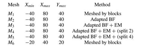
Table 3. Comparison of the performance of several meshes at  $Re_c = 170$.
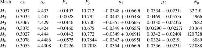
Appendix E: Three-dimensional stability of steady-state solutions
In this section, we review three-dimensional stability studies carried out by Pralits et al. (Reference Pralits, Giannetti and Brandt2013), Rao et al. (Reference Rao, Leontini, Thompson and Hourigan2013a,Reference Rao, Leontini, Thompson and Houriganb), Radi et al. (Reference Radi, Thompson, Rao, Hourigan and Sheridan2013) and Rao et al. (Reference Rao, Radi, Leontini, Thompson, Sheridan and Hourigan2015).
It is now well known the secondary three-dimensional transition from a two-dimensional unsteady flow towards a three-dimensional flow at  $Re \approx 190$ and $\alpha =0$, see Williamson (Reference Williamson1996). Vortices in the wake of the fixed cylinder, i.e. $\alpha =0$, develop spanwise waviness whose wavelength is approximatelyfour cylinder diameters. The rotation of the cylinder surface on this linear steady mode, denoted as Mode A in Rao et al. (Reference Rao, Radi, Leontini, Thompson, Sheridan and Hourigan2015), has a stabilising effect for rotation rates $\alpha < 1$, see figure 12.
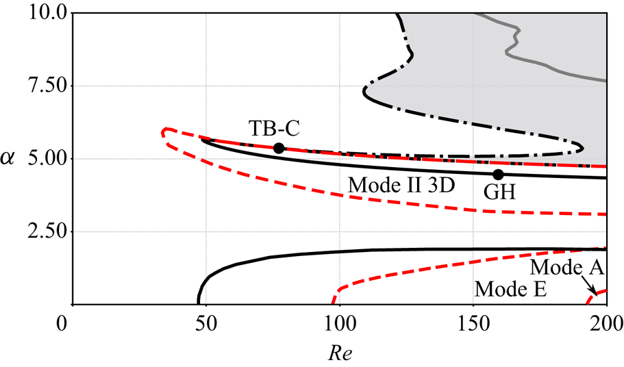
Figure 12. Neutral stability curves in the range  $Re \in [0,200]$ and $\alpha \in {[ 0,10 ]}$. Black and grey lines are used to denote two-dimensional local bifurcations whereas red lines are used to designate the boundaries of three-dimensional local bifurcations. Dashed and point-dashed lines indicate the presence of a stationary bifurcation boundary, solid lines are used to designate unsteady bifurcation boundaries.
Instead, if we consider the stability of an infinitesimal spanwise perturbation on a steady-state solution, the flow displays spanwise waviness at a much lower Reynolds number  $Re\approx 100$ and $\alpha =0$. The onset of instability of this stationary mode, denoted as Mode E in Rao et al. (Reference Rao, Radi, Leontini, Thompson, Sheridan and Hourigan2015), is shown in figure 12 as a function of $(Re,\alpha )$.
In the same region of existence of the unsteady two-dimensional Mode II, experimental evidence has shown the presence of a three-dimensional mode, see Linh (Reference Linh2011). A steady three-dimensional mode, here denoted as Mode II-3D, extends to lower Reynolds values than the two-dimensional threshold of the non-rotating cylinder, and for a larger interval in  $\alpha$ than the two-dimensional Mode II. The instability mechanism of Mode II-3D is of hyperbolic nature, see Pralits et al. (Reference Pralits, Giannetti and Brandt2013).
Finally, note that the occurrence of two unstable modes has also been documented in the flow past rotating spheres (Citro et al. Reference Citro, Tchoufag, Fabre, Giannetti and Luchini2016; Fabre et al. Reference Fabre, Tchoufag, Citro, Giannetti and Luchini2017). However, the spatial structure of the direct and adjoint modes for our geometrical configuration is very different with respect to the case of the rotating sphere flow.


 Open access