2.1 Jet facility

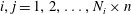
Experiments were conducted in a round air jet facility, as schematically shown in figure 1. The facility was placed in an air-conditioned laboratory where the room temperature remains constant within $\pm 0.5^{\circ }\text{C}$ , centrally deployed in an area of approximately 2.5 m in width and 2 m in height, enclosed by fabric walls. In order to minimize the effects of the wall on the jet, the nozzle exit is 4.0 m away from the fabric partition wall and the distance is well over 70 times the jet exit diameter required for neglecting the wall effects (Malmstrom et al. Reference Malmstrom, Kirkpatrick, Christensen and Knappmiller1997). As the jet is highly sensitive to background noise, careful measures are taken to avoid any external interference to airflow.

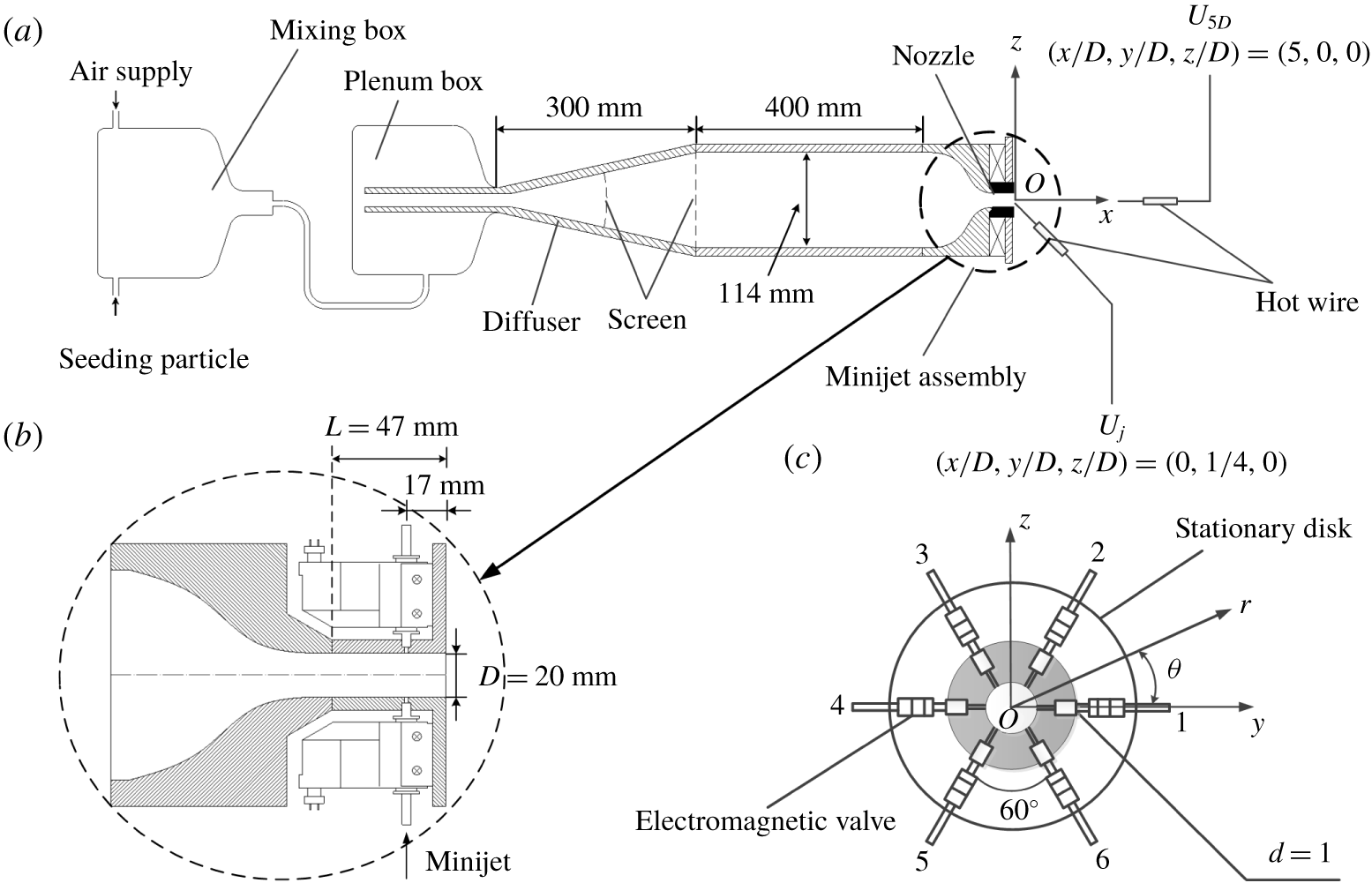
Figure 1. Sketch of the experimental setup: (a) main jet facility; (b) minijet assembly; (c) minijet arrangement.

The compressed air of the round jet comes from a constant 5 bar gauge pressure, mixed with seeding particles in the mixing chamber in the case of the particle image velocimetry (PIV) or flow visualization measurements, and then enters into a plenum chamber, composed of a 300 mm long diffuser of $15^{\circ }$ in half-angle and a 400 mm long cylindrical settling chamber with an inner diameter of 114 mm. The flow passes two screens before entering the smooth contraction nozzle (Perumal & Zhou Reference Perumal and Zhou2018), which is extended by a 47 mm long smooth tube of the same diameter as the nozzle exit $D\,(=20~\text{mm})$ . The Reynolds number $Re_{D}=\overline{U}_{j}D/\unicode[STIX]{x1D708}$ of the main jet is fixed at 8000, where $U_{j}$ is the centreline velocity measured at the nozzle exit, the overbar denotes time-averaging and $\unicode[STIX]{x1D708}$ is the kinematic viscosity of air. A Cartesian coordinate system ( $x,y,z$ ) is defined in figure 1(a,c), with its origin at the centre of the jet exit and the $x$ -axis pointing in the direction of flow. Measurements were conducted in the $x$ – $z$ , $x$ – $y$ and $y$ – $z$ planes of the main jet. The instantaneous and fluctuating velocities in the $x$ , $y$ and $z$ directions are denoted by ( $U,V,W$ ) and ( $u,v,w$ ), respectively.

Six unsteady control minijets issued from orifices with a diameter of 1 mm are equidistantly placed around the extension tube at $x_{i}=-0.85D$ , $y_{i}=(D/2)\cos \unicode[STIX]{x1D703}_{i}$ , $zi=(D/2)\unicode[STIX]{x1D703}_{i}$ , where $\unicode[STIX]{x1D703}_{i}=(i-1)2\unicode[STIX]{x03C0}/6$ , $i=1,2,\ldots ,6$ (figure 1 b,c). Their mass flow rate is determined by a flow-limiting valve and monitored by a mass flow meter, with a measurement uncertainty of 1 %, and the frequencies and duty cycles are independently controlled by individual electromagnetic valves that are operated in an ON/OFF mode. The maximum operating frequency of the valves is 500 Hz, exceeding three times the preferred-mode frequency, $f_{0}=135~\text{Hz}$ , of the unforced jet, the corresponding Strouhal number being 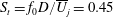$S_{t}=f_{0}D/\overline{U}_{j}=0.45$ , where $f_{0}$ is obtained from the power spectral density function $E_{u}$ of the streamwise fluctuating velocity $u$ measured in the absence of control (Yang & Zhou Reference Yang and Zhou2016).

2.2 Flow measurements

The fluctuating flow velocities are monitored by two tungsten wire sensors of $5~\unicode[STIX]{x03BC}\text{m}$ in diameter, operated on a constant temperature circuit (Dantec streamline) at an overheat ratio of 0.6, one placed at $(x/D,y/D,z/D)=(0,1/4,0)$ and the other at $(x/D,y/D,z/D)=(5,0,0)$ . The time-averaged velocity at the latter position is denoted by $U_{5D}$ . This choice is based on the following considerations. Firstly, Zhou et al. (Reference Zhou, Du, Mi and Wang2012) demonstrated that the decay rate of the centreline mean velocity of jet defined by 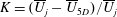$K=(\overline{U}_{j}-\overline{U}_{5D})/\overline{U}_{j}$ is correlated approximately linearly with an equivalent jet half-width $R_{eq}=[R_{H}R_{V}]^{0.5}$ , where $R_{H}$ and $R_{V}$ are the jet half-widths in two orthogonal planes, implying that $K$ is directly connected to the entrainment rate of the manipulated jet. Secondly, Fan et al. (Reference Fan, Wu, Yang, Li and Zhou2017) found that the difference $\triangle K$ between the $K$ values with and without control reaches the maximum at $x/D\approx 5$ , that is, the centreline mean streamwise velocity measured at $x/D=5$ is most sensitive to the change in the control parameters. Finally, the variation in $K$ is almost linear from $x/D=0$ to $x/D\approx 7$ under control (figure 7, Fan et al. (Reference Fan, Wu, Yang, Li and Zhou2017)), that is, a single value of $K$ may be used to describe reasonably well the jet decay rate in the near field under control. Both hot wires are calibrated at the jet exit using a pitot-static tube connected to a micromanometer (Furness Controls FCO510). The cutoff and sampling frequencies are 3 kHz and 6 kHz for open-loop control experiments, respectively. The experimental uncertainty of the hot-wire measurement is estimated to be less than 2 %.

A planar high-speed PIV system, with a high-speed camera (Dantec speed sensor 90C10, $2056\times 2056$ pixels resolution) and a pulsed laser source (Litron LDY304-PIV, Nd: YLF, $30~\text{mJ}~\text{pulse}^{-1}$ ), is deployed for velocity field measurements in the $x$ – $z$ , $x$ – $y$ and $y$ – $z$ planes. An oil droplet generator (TSI MCM-30) is used to generate fog from olive oil with an averaged particle size of $1~\unicode[STIX]{x03BC}\text{m}$ for flow seeding. Flow illumination is provided by a laser sheet of 1 mm in thickness generated by the pulsed laser via a cylindrical lens. For velocity measurements in the $x$ – $z$ and $x$ – $y$ planes, the captured image covers the area of $x/D\in [0,6]$ and $y/D$ , $z/D\in [-2,2]$ . The longitudinal and lateral image magnifications are identical, 0.09 mm per pixel. The time interval between two consecutive images is presently chosen to be $25~\unicode[STIX]{x03BC}\text{s}$ , which is found to yield satisfactory results. There are $253\times 253$ velocity vectors, the same for the two planes. A total of 200 pairs of flow images are captured at a sampling rate of 405 Hz for each set of PIV data. In post-processing, a built-in adaptive correlation function of the flow map processor (PIV 2001 type) is applied with an interrogation window of $32\times 32$ pixels and a 75 % overlap along both directions.

The same PIV system is used for flow visualization in the three orthogonal planes. So are the seeding particles, though their concentration is higher than in the PIV measurements to provide a clear picture for the flow structure. The captured images cover the area of $x/D\in [0,6]$ and $y/D$ or $z/D\in [-2,2]$ in the $x$ – $y$ and $x$ – $z$ planes and the area of $y/D=z/D\in [-2,2]$ at $x/D=0.25$ in the $y$ – $z$ plane.

2.3 Real-time system

A national instrument PXIe-6356 multifunction I/O device, connected to a computer, is used in experiments to generate the real-time control command at a sampling rate of $F_{rf}=1~\text{kHz}$ . A LabVIEW real-time module is used to execute the program. Sensor data acquisition and control command generation for the AI control experiments are operated under the same sampling frequency of 1 kHz. It has been confirmed that the ON/OFF command lasts at least 1 ms to ensure the actuators work effectively. The available $f_{a}$ can be derived from $f_{a}=F_{rf}/N_{sp}$ , where $N_{sp}$ is the number of sampling points in one period $1/f_{a}$ . The working frequency range of actuators [0, 500 Hz] imposes a minimum value for $N_{sp}$ , i.e.  $N_{sp}\geqslant 2$ . For a given frequency, $\unicode[STIX]{x1D6FC}$ can be deduced from $m/N_{sp}$ , $m=1,\ldots ,N_{sp}-1$ . The $m$ range ensures a response time of 1 ms for the effective working of the actuators, which is adequate as the maximum sampling rate $F_{rf}$ is 1 kHz due to the limitation of hardware. Thus, the number of possible duty cycles $N_{\unicode[STIX]{x1D6FC}}$ for a given $f_{a}$ is $N_{\unicode[STIX]{x1D6FC}}=N_{sp}-1=F_{rf}/f_{a}-1$ , which increases with $F_{rf}$ and decreases with $f_{a}$ . This process is similar to the one used by Li et al. (Reference Li, Noack, Cordier, Borée, Kaiser and Harambat2017) and Wu et al. (Reference Wu, Fan, Zhou, Li and Noack2018a ).

3.1 Minijet-produced flow

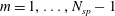
It is important to document the flow produced by a minijet and the effect of minijets on the initial condition of the main jet. This information is crucial for understanding physically the manipulated jet. The instantaneous velocity $U_{a}$ of a single radial minijet is first examined in the absence of the main jet. A hot wire is placed 17 mm or $x/D=-0.85$ upstream of the main jet exit and 3 mm radially from the exit of minijet 1 (figure 1 c). The hot wire is oriented normal to the minijet axis – recording the signal $U_{a}$ , which changes with $\unicode[STIX]{x1D6FC}$ (figure 2). For $\unicode[STIX]{x1D6FC}=0.1$ , $U_{a}$ displays sharp peaks which are periodic and clearly separated. But these peaks are less pronounced at $\unicode[STIX]{x1D6FC}=0.4$ . The signal $U_{a}$ is almost steady at $\unicode[STIX]{x1D6FC}=1$ , though showing a small variation, as observed by Johari, Pachecotougas & Hermanson (Reference Johari, Pachecotougas and Hermanson1999). Apparently, a small $\unicode[STIX]{x1D6FC}$ produces a large instantaneous velocity, implying a large penetration depth into the main jet.

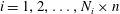
Figure 2. Time histories of minijet injection velocity $U_{a}$ at duty cycles $\unicode[STIX]{x1D6FC}=0.1$ , 0.4 and 1 (see legend) in the absence of the main jet measured at $(x/D,y/D,z/D)=(-0.85,-0.35,0)$ for $C_{m}=1.2\,\%$ , $f_{a}/f_{0}=0.5$ . $\overline{U_{j}}=0$ .

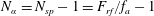
Figure 3. Time histories of two minijet injection velocity signals $U_{a1}$ , $U_{a2}$ measured simultaneously at $(x/D,y/D,z/D)=(-0.85,\pm 0.35,0)$ for $C_{m}=1.2\,\%$ , $f_{a}/f_{0}=0.5$ and $\unicode[STIX]{x1D6FC}=0.1$ . There is a phase difference $\unicode[STIX]{x1D6F7}$ between two minijets control signals: (a–b)  $\unicode[STIX]{x1D6F7}=0$ , (c–d)  $\unicode[STIX]{x1D6F7}=60^{\circ }$ , (e–f)  $\unicode[STIX]{x1D6F7}=180^{\circ }$ . $\overline{U}_{j}=0$ .

Consider the simultaneous injection of minijets 1 and 4 (figure 1 c) without the main jet. Two hot wires are placed perpendicularly to the $x$ – $y$ plane at $x/D=-0.85$ and 3 mm from each of the corresponding measured minijet exit. The two minijets are injected with a phase shift $\unicode[STIX]{x1D6F7}$ , which may be varied by changing the phase shift between the two square wave signals of input voltages. At $\unicode[STIX]{x1D6F7}=0^{\circ }$ , the $U_{a1}$ signal exhibits a very sharp peak value, with a magnitude of close to 0 at the off-state of the minijet and about 13 at the on-state (figure 3 a). Note that, even after the electromagnetic valve is closed, there may be some fluid injecting into the main jet (Sailor, Rohli & Fu Reference Sailor, Rohli and Fu1999). A similar observation can be made for $\unicode[STIX]{x1D6F7}=60^{\circ }$ and $180^{\circ }$ (figure 3 b,c). The characteristics of $U_{a2}$ resemble those of $U_{a1}$ , regardless of the $\unicode[STIX]{x1D6F7}$ value. It may be inferred that each of the minijets does not depend on $\unicode[STIX]{x1D6F7}$ and is rather independent of each other.

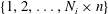
Figure 4. Typical hot-wire signals of instantaneous streamwise velocity $U/\overline{U_{j}}$ along $x$ – $y$ plane at $x/D=0.05$ for minijet numbers $N=1$ , 3, 4 and 6 ( $f_{a}/f_{0}=0.5$ , $\unicode[STIX]{x1D6FC}=0.15$ , $C_{m}=1.2\,\%$ ). The same scale is applied for all signals. The dots within the circle represent the hot-wire measurement points.

3.2 Penetration depth and minijet number

The penetration depth of control jets may have a pronounced impact upon jet mixing (Davis Reference Davis1982). Thus, its influence on the main jet is examined for various minijet numbers and configurations with given $\overline{U}_{j}$ and control parameters, i.e.  $\unicode[STIX]{x1D6FC}$ , $f_{a}/f_{0}$ and mass flow ratio $C_{m}=m_{mini}/m_{j}$ , where $m_{mini}$ and $m_{j}$ are the mass flow rates of a single minijet and main jet, respectively. The minijet penetration depth could be approximately estimated from the $U$ signals along the $y$ -direction, measured at $x/D=0.05$ using a hot wire placed perpendicularly to the $x$ – $y$ plane, as shown in figure 4, where the scale of the abscissa or ordinate is made the same for all cases to facilitate comparison. The $U$ signals are essentially constant throughout the range of $y/D$ $\in$ [ $-0.3$ , 0.3] for the unforced jet. The periodic fluctuations of $U$ appear at $y/D=-0.3$ for one minijet injection $(N=1)$ , and its magnitude grows first and then retreats with increasing $y/D$ . The fluctuations remain discernible at $y/D=-0.1$ . Note that the minijet is issued along the $y$ -direction. Beyond $y/D=-0.1$ , the velocity fluctuations are negligibly small and in fact comparable to that in the unforced jet. These observations indicate that the minijet has reached a penetration depth of $y/D=-0.1$ . With three adjacent minijets on $(N=3)$ , the velocity fluctuations are appreciably larger in magnitude than their counterparts of $N=1$ , and the maximum amplitude is shifted to a deeper position, i.e. from $y/D=-0.1$ at $N=1$ to $y/D=0$ at $N=3$ . The fluctuations are now discernible at $y/D=0.2$ , indicating an increased penetration depth, though the minijets clearly have not impinged on the wall opposite to the injecting minijets. With $N$ increasing to 4, the maximum magnitude of the velocity fluctuations is appreciably larger than that of $N=3$ , and again occurs at the centre $(y/D=0)$ , where all minijets contribute to an increase in the velocity fluctuations. Furthermore, the fluctuations are now even discernible at $y/D=0.3$ . It is worth pointing out that we did not move the hot wire closer to the wall because of its high fragility; therefore, we could not tell whether the minijets have penetrated through the main jet in this case. At $N=6$ , the velocity fluctuations display symmetry about the centre, the maximum magnitude exceeding all other cases and taking place at the centre.

3.3 Power spectral density function and minijet number

Figure 5 compares $E_{u}$ measured on the centreline at $x/D=0.05$ with and without the main jet operated, where the log–log scale is used to emphasize the low-frequency components. This function $E_{u}$ yields $\overline{u^{2}}=\int _{0}^{\infty }E_{u}\,\text{d}f$ , where $f$ is frequency. In figure 5 e, $E_{u}$ measured in the unforced jet shows a pronounced peak at $f_{0}$ , indicating clearly the occurrence of the preferred mode structure. When the minijets as well as the main jet are operated, $E_{u}$ exhibits more pronounced peaks at $f/f_{a}=1$ and its harmonics. These observations result from the interaction between the main jet and minijet, referred to as the parametric resonance by Huang & Hsiao (Reference Huang and Hsiao1999). Evidently, the unsteady injection produces the periodic structures upstream of the nozzle exit, as noted by Zhou et al. (Reference Zhou, Du, Mi and Wang2012). With increasing $N$ , the peaks become more pronounced and occur at more harmonics, echoing the enhanced periodic structures (figure 4) and, hence, the enhanced excitation of the shear layer. The predominant frequencies do not vary with $N$ though. Note that $E_{u}$ is normalized by $\overline{u^{2}}$ so that its integration over the entire frequency range is always equal to unity. As a result, $E_{u}$ drops appreciably over the low frequency range.

Figure 5. Power spectral density function $E_{u}$ of hot-wire signals $u$ measured at $(x/D,y/D,z/D)=(0.05,0,0)$ with and without the main jet: (a)  $N=1$ , (b)  $N=3$ , (c)  $N=4$ , (d)  $N=6$ , (e)  $N=0$ , $(x/D,y/D,z/D)=(3,0,0)$ .

3.4 Fluctuating velocity and minijet number

The number and configuration of minijets may profoundly affect the main jet issuing from the nozzle, as in the case of passive delta tabs (Zaman et al. Reference Zaman, Reeder and Samimy1994). This effect plays an important role in the downstream evolution of flow. As such, the radial profiles of the hot-wire measured root-mean-square (r.m.s.) velocity $u_{rms}$ at $x/D=0.05$ are examined in the manipulated jets, along the $y$ and $z$ axes, respectively, for $N=1$ , 2, 3, 6. The data of the unforced jet are also presented for the purpose of comparison. Given the symmetrically arranged minijets ( $N=2$ , 6) about the $x$ – $z$ plane (figure 6 b1,d1), the $u_{rms}$ distributions along the $y$ -axis exhibit reasonable symmetry. The $u_{rms}$ displays a pronounced peak at about $y/D=\pm 0.45$ , where the shear layer is expected, in the injection or $x$ – $y$ plane for $N=2$ (figure 6 b1), but remains unchanged in the orthogonal or $x$ – $z$ plane (figure 6 b2), indicating that the shear layer between the two minijets is essentially undisturbed. Being symmetrical about the $z$ -axis, the $u_{rms}$ distributions are given only for $z/D\geqslant$ 0 in figure 6(a2–d2). A broad bump is evident at $y/D\approx 0.2$ for $N=2$ (figure 6 b1). The flow structure induced by an unsteady injecting minijet is similar to a pulsed jet in cross-flow, which forms a series of periodical vortex rings (M’closkey, King & Cortelezzi Reference M’closkey, King and Cortelezzi2002). It seems that these minijet-produced periodic vortices may occur most likely at $y/D\approx$ 0.2, accounting for the broad bump. For $N=3$ and 6, this bump moves to near the centre, with a significantly increased magnitude (figure 6 c1,d1). Two factors may be responsible for this increase. Firstly, as the separation angle $\unicode[STIX]{x1D703}$ decreases from 180 $^{\circ }$ to 120 $^{\circ }$ and then 60 $^{\circ }$ , two neighbouring minijets become close and their induced unsteady flows interact more and more intensely. Zaman et al. (Reference Zaman, Reeder and Samimy1994) noted that, as the neighbouring delta tabs approach each other, streamwise vortices interact more vigorously, resulting in the jet core fluid ejection. Secondly, as demonstrated in figure 4, every minijet generates a velocity fluctuation at the centre. For $N=6$ , $\unicode[STIX]{x1D703}$ is smallest and all six minijets contribute to flow perturbations, thus producing the most pronounced bump at $y/D=0$ .

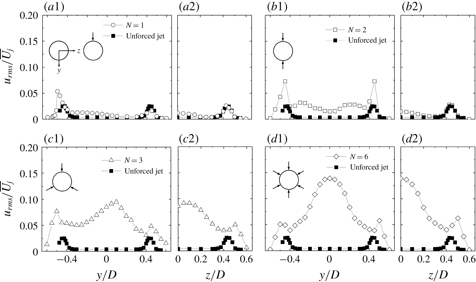
Figure 6. Radial distributions of fluctuating velocity $u_{rms}/\overline{U_{j}}$ measured at $x/D=0.05$ ( $f_{e}/f_{0}=0.5$ , $C_{m}=1.2\,\%$ ) depend on minijet number: (a1–d1) along the $y$ -axis, (a2–d2) along the $z$ -axis.

4.1 Artificial intelligence control system

Artificial intelligence methods allow us to explore the rich universe of nonlinear actuation mechanisms opened by independent spatially distributed actuators. Hence, we see the actuation and sensing hardware and control logic as intimately interwoven. The AI control system is sketched in figure 7. Generally, a control system facilitates a control goal for a plant by control hardware and a control logic/controller. The control hardware includes sensors and actuators as discussed in § 2. This hardware monitors the plant output (velocity signals) and executes instructions from the controller. The open-loop arrangement is shown in figure 1(a) for calculating the cost value $J=\overline{U}_{5D}/\overline{U}_{j}$ . A minimized cost $J$ corresponds to the maximized decay rate $K=1-J$ of jet centreline mean velocity, which is an indicator of the mixing efficacy of a jet (Perumal & Zhou Reference Perumal and Zhou2018).

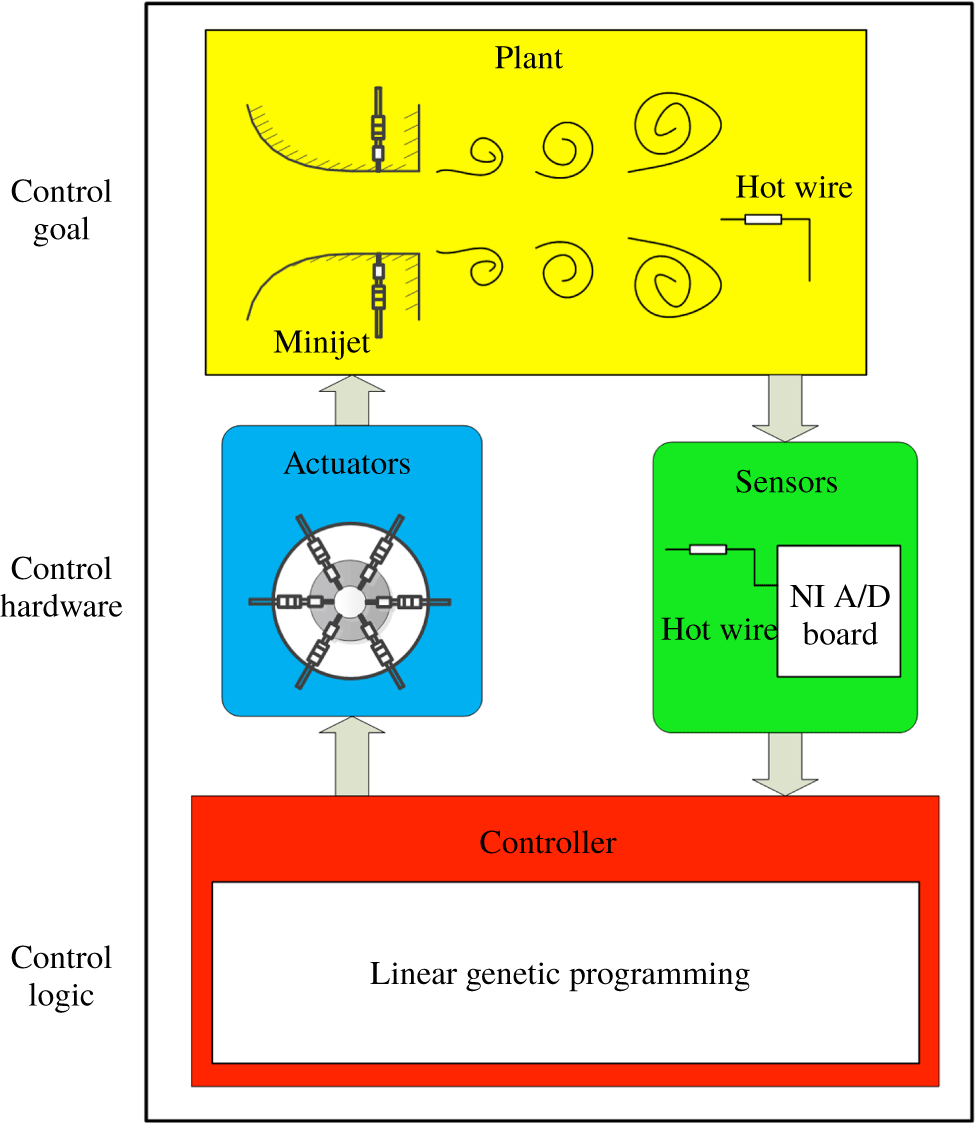
Figure 7. Principle sketch of the artificial intelligence control which consists of a plant (yellow), sensors (green), actuators (blue) and a controller (red) that includes a linear genetic programming (LGP) algorithm or other machine learning methods.

4.2 Control optimization using linear genetic programming

The six-dimensional vector $\boldsymbol{b}=[b_{1},b_{2},\ldots ,b_{6}]^{\dagger }$ comprises all actuation commands. The $i$ th minijet is ‘ON’ if the actuation command $b_{i}$ is positive and is ‘OFF’ otherwise. In the sequel, we assume that $b_{i}=1$ for ‘ON’ and $b_{i}=0$ for ‘OFF’. Following Wu et al. 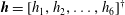(Reference Wu, Fan, Zhou, Li and Noack2018a ), we search for a control law including sensor feedback with hot-wire signals $\boldsymbol{s}$ , multi-frequency open-loop forcing with harmonic functions contained in $\boldsymbol{h}=[h_{1},h_{2},\ldots ,h_{6}]^{\dagger }$ . Here, 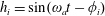$h_{i}=\sin (\unicode[STIX]{x1D714}_{a}t-\unicode[STIX]{x1D719}_{i})$ , $i=1,2,\ldots ,6$ , where $t$ is time, $\unicode[STIX]{x1D714}_{a}$ is a reference frequency to be determined in § 5.1 and $\unicode[STIX]{x1D719}_{i}$ is the phase. Then,

where the vector function $\boldsymbol{K}=[K_{1},\ldots ,K_{6}]$ comprises the actuation laws for each minijet. The time-averaged duty cycle of the $i$ th minijet is determined by the control law $\boldsymbol{K}$ and the arguments, i.e. sensor signals and harmonic functions. For open-loop forcing $\boldsymbol{b}=\boldsymbol{K}(\boldsymbol{h})$ , the duty cycle of the $i$ th minijet becomes the sensor-independent time-average of the actuation command $\overline{K}_{i}(h)$ . Thus, helical forcing may have a particularly simple representation, e.g.  $b_{i}=h_{i}$ . In general, only two harmonic functions, typically $\sin \unicode[STIX]{x1D714}_{a}t$ and $\cos \unicode[STIX]{x1D714}_{a}t$ , are sufficient for harmonic functions with arbitrary phases. Following Paschereit, Wygnanski & Fiedler (Reference Paschereit, Wygnanski and Fiedler1995) and others, we add the cosine and sine components of $\unicode[STIX]{x1D714}_{a}/2$ and $\unicode[STIX]{x1D714}_{a}/4$ , yielding a ten-dimensional vector $h=[h_{1},h_{2},\ldots ,h_{10}]^{\dagger }$ . The nonlinear function $\boldsymbol{K}$ can create arbitrary higher harmonics, arbitrary phase relationships between $\unicode[STIX]{x1D714}_{a}$ , $\unicode[STIX]{x1D714}_{a}/2$ , $\unicode[STIX]{x1D714}_{a}/4$ and higher harmonics, e.g.  $1-2h^{10}=\cos (10\unicode[STIX]{x1D714}_{a}t)$ , as well as arbitrary sum and difference frequencies. The control optimization searches for a law of form (4.1) that minimizes the cost,

The regression problem implies a search for a mapping from multiple inputs to a multiple-output signal. Even in case of a linear function this implies the optimization of a large number of parameters. We employ the powerful linear genetic programming (LGP) as a regression solver and take the same parameters for the control law representation and for the genetic operations as Wu et al. (Reference Wu, Fan, Zhou, Li and Noack2018a ). The first generation of LGP, $n=1$ , contains $N_{i}=100$ random control laws, also called individuals. Each individual ‘ $i$ ’ is experimentally tested for 5 s to yield the measured cost $J_{i}^{n}$ , where the superscript ‘ $n$ ’ denotes the generation number. Subsequent generations are produced from the previous ones with genetic operations (elitism, crossover, mutation and replication) and tested analogously. In the case of elitism, top-ranking individuals pass directly to the next generation. Replication copies a stochastically selected number of individuals into the next generation, which acts to preserve some well performing individuals. Crossover involves two selected individuals and then produces two individuals, with part of their elements exchanged. This operation tends to generate better individuals by exploitation. For the mutation operation, the instructions of a selected individual are randomly changed. Both crossover and mutation serve to explore potentially new and better minima of $J$ . After the in situ performance measurements, the individuals are renumbered in order of performance, $J_{1}^{n}\leqslant J_{2}^{n}\leqslant \cdots \leqslant J_{N_{i}}^{n}$ , where the subscript $i$ represents the individual index and $N_{i}$ and $n$ respectively denote the size and number of generations. We have noted in trial tests that all the winning individuals always involve every actuator. Therefore, when generating the 100 individuals of the first generation, we exclude the possibility of a permanently inactive actuator to accelerate the learning process, that is, as a plant-specific rule, we discard and replace any individual for testing if one or more actuators are not active.

It is worth mentioning that the present jet control is formulated as a model-free regression problem: determine the law which minimizes the given cost function. The considered search space of control laws significantly extends hitherto considered actuations. Firstly, general multiple-input actuation is allowed without any imposed symmetry constraints. Thus, actuations with arbitrary combinations of minijets thereof can be realized. Secondly, the search space includes broadband multi-frequency actuation. Thirdly, nonlinear sensor feedback is included, which is made by nonlinear operations with the sensor signal $\boldsymbol{s}$ , e.g.  $\boldsymbol{b}=\log _{10}(\boldsymbol{s})$ (Wu et al. Reference Wu, Fan, Zhou, Li and Noack2018a ). However, this feature is not found improving appreciably the control performance and is therefore removed eventually in the learning process. Fourthly, the control law may include nonlinear combinations of multi-frequency forcing and sensor feedback. The key enabler for the control optimization in this search space is genetic programming as a powerful regression solver. Genetic programming may be considered as an example for the many powerful regression solvers of AI.

4.3 Parameters and control landscape

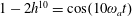
The LGP parameters for this study are displayed in table 1. These values are adopted from a previous MLC jet mixing study in the same facility with a single minijet (Wu et al. Reference Wu, Fan, Zhou, Li and Noack2018a ). The parameters are identical or close to the ones employed in numerous experimental studies as summarized by Duriez et al. (Reference Duriez, Brunton and Noack2016) and Noack (Reference Noack, Zhou, Kimura, Peng, Lucey and Hung2019). Elitism is set to $N_{e}=1$ , i.e. the best individual of a generation is copied to the next one. The replication, crossover and mutation probabilities are $10\,\%,70\,\%$ and $20\,\%$ , respectively. The individuals on which these genetic operations are performed come from a tournament selection of size $N_{t}=7$ . The instruction number varies from 10 to 50. The operations comprise $+,-,\times ,\div ,\sin ,\cos ,\tanh ,\log _{10}$ and $g^{2}$ , where $g$ is the input argument. The operations $\div$ and $\log _{10}$ are protected to prevent an undefined expression with a vanishing argument; for example, $\log _{10}(g)$ is modified to $\log _{10}(|g|)$ . In addition, LGP uses three random constants in the range $[-1,1]$ .

The evolution of control laws is depicted with a proximity map following Duriez et al. (Reference Duriez, Brunton and Noack2016). The main idea is that the considered ensemble of $\boldsymbol{K}_{i}(\boldsymbol{h})$ is represented as points in a two-dimensional feature plane $\unicode[STIX]{x1D738}_{i}=(\unicode[STIX]{x1D6FE}_{i,1},\unicode[STIX]{x1D6FE}_{i,2})$ , where $i=1,2,\ldots ,N_{i}\times n$ , so that the difference between the control laws is optimally indicated by the distance between feature vectors. The key is the definition of a metric $D_{ij}$ between the control laws $\boldsymbol{K}_{i}(\boldsymbol{h})$ and $\boldsymbol{K}_{j}(\boldsymbol{h})$ . For the considered open-loop actuation, this metric is the root-mean-square averaged Euclidean difference between the actuation command vectors accounting for a potential time-delay, given by

In the employed metric, we incorporate also the control performance $J_{i}$ by a penalization term, i.e.

The parameter $\unicode[STIX]{x1D6FD}$ is chosen so that the maximum actuation distance $M_{ij}$ is equal to the maximum difference in the performance terms:

Given the resulting configuration matrix $\unicode[STIX]{x1D63F}=(D_{ij})$ ( $i,j=1,2,\ldots ,N_{i}\times n$ ), classical multi-dimensional scaling (Cox & Cox Reference Cox and Cox2000) uniquely determines feature vectors $\unicode[STIX]{x1D738}_{i}$ , $i=1,2,\ldots ,N_{i}\times n$ , so that the distances are optimally preserved:

The translational degree of freedom is removed by centring the feature vectors $\sum _{i=1}^{N_{i}\times n}\unicode[STIX]{x1D738}_{i}=0$ . The feature vectors are sorted and rotated so that the first coordinate has the largest variance, the second coordinate the second largest, etc. The coordinates are indeterminate by a sign (mirroring), like POD modes and their amplitudes.

Finally, a control landscape $J(\unicode[STIX]{x1D738})$ is interpolated from the three-dimensional data points ( $\unicode[STIX]{x1D6FE}_{i,1},\unicode[STIX]{x1D6FE}_{i,2},J_{i}$ ), $i=1,2,\ldots ,N_{i}\times n$ . The two-dimensional feature vectors $\unicode[STIX]{x1D738}_{i}$ are connected by an unstructured grid from a Delaunay (Reference Delaunay1934) triangulation. This triangulation guarantees that the mesh triangles are optimally equilateral. The $J$ -values in each mesh triangle $i_{1},i_{2},i_{3}$ $\in$ $\{1,2,\ldots ,N_{i}\times n\}$ are interpolated from the known values at the vertices $J_{i_{1}},J_{i_{2}},J_{i_{3}}$ . These control landscapes have been employed in several AI-based control schemes (Kaiser et al. Reference Kaiser, Noack, Spohn, Cattafesta and Morzyński2017). They indicate the complexity of the actuation response and the learning progress of AI-based control. Often, the feature coordinates can be linked with the physical properties of actuation a posteriori, thus providing additional insights.

5.1 Representative reference actuations

A few well-known reference forcings are firstly presented to facilitate the understanding of the AI learning process and highlight the uniqueness of this method. In our earlier studies, turbulent jet mixing has been optimized for the same cost function and experimental conditions. For single unsteady minijet forcing, the optimal $f_{a}$ is found to be 67 Hz (Wu et al. Reference Wu, Fan, Zhou, Li and Noack2018a ), $0.5f_{0}$ , and the optimal $C_{m}$ is 1.2 % based on a dual-input-and-one-output closed-loop control technique (Wu, Wong & Zhou Reference Wu, Wong and Zhou2018b ). As such, we choose the same $f_{a}$ or $\unicode[STIX]{x1D714}_{a}=2\unicode[STIX]{x03C0}f_{a}$ and $C_{m}=1.2\,\%$ for every minijet. With $C_{m}$ fixed for each minijet, the overall mass flow of injected fluid in one actuation period $T_{a}$ is the same for all actuations, that is, the input/actuation energy is the same, irrespective of control modes or laws. Consider three reference forcings (e.g. Hilgers & Boersma Reference Hilgers and Boersma2001; Yang & Zhou Reference Yang and Zhou2016; Yang Reference Yang2017), viz.

The constants $\unicode[STIX]{x1D6FC}_{a}$ , $\unicode[STIX]{x1D6FC}_{h}$ and $\unicode[STIX]{x1D6FC}_{f}$ correspond to the duty cycles and have been optimized with respect to the cost. As mentioned before, actuation is performed only when $b_{i}>0$ . The cost functions are found to be $J_{a}=0.665$ , $J_{h}=0.568$ and $J_{f}=0.423$ for the optimized axisymmetric, helical and flapping forcings (table 2), respectively, based on the conventional open-loop control, which provide the benchmarks for the AI control performance to be discussed below.

5.2 Learning process of AI control

In the initial stage of the learning process we included a feedback signal $\boldsymbol{s}(t)=[u_{3D},u_{5D}]$ as one input (equation (4.1)) for the AI system, where $u_{3D}$ and $u_{5D}$ are the fluctuating velocity signals measured at $x/D=3$ and 5, respectively. It is found from dozens of experiments that the search for the optimal solution benefits neither from the subharmonic components of $h_{7},\ldots ,h_{10}$ nor from the feedback signals. Therefore, the AI control laws (4.1) may be cast in the periodic open-loop form, 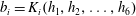$b_{i}=K_{i}(h_{1},h_{2},\ldots ,h_{6})$ , $i=1,2,\ldots ,6$ . Hence, we restrict our following discussion to this open-loop actuation.

Figure 8. Learning curve ( $3000$ individuals) of AI control for ( $u$ ) unforced jet, ( $a$ ) axisymmetric forcing, ( $h$ ) helical forcing, ( $f$ ) flapping forcing and ( $c$ ) combined forcings. Here $J_{u}$ , $J_{a}$ , $J_{h}$ and $J_{f}$ are costs corresponding to the benchmarks of unforced, open-loop axisymmetric, helical and flapping forcings, respectively (see table 2).

The learning curve of the AI control is presented in figure 8, where the square symbol marks the first and best individual of each generation with $N_{i}=100$ control laws. The remaining costs grow monotonously with their indices, and the 100 individuals of each generation form a colour bar. The square symbol curve unveils the best performance from generation $n=1$ to 30. The best individual of the first generation or stage 1 is characterized by an axisymmetric control law (see (A 1) in appendix A).

This law is equivalent to (5.1a ) except for a time shift, reflected by $4/6\unicode[STIX]{x03C0}$ . The performance $J_{1}^{1}=0.626$ (see figure 8 and table 2) is slightly better, about 5.8 % lower, than the benchmark of axisymmetric forcing (5.1a ), though much higher than that ( $J_{u}=0.947$ or $K\approx 0.05$ ) of the unforced jet. Note that the centreline mean velocity for calculating $K$ or $J_{a}$ is measured over a duration of 60 s in the benchmark experiments, but only 5 s for estimating $J_{i}$ as the measured $J_{i}$ is used to evaluate control laws and does not need to be very accurate in the learning process of AI control. An accurate long-time evaluation of $J$ is performed only in the last generation $n=30$ . This difference in evaluating the cost function could account for the deviation between $J_{1}^{1}$ and $J_{a}$ . However, the AI control or specifically genetic programming breeds several copies of the winning individual, covering all possible combinations of the control parameters, and then takes the best performing one. This process differs in essence from the searching process of the conventional open-loop control which optimizes one control parameter first and then moves to next with the first parameter fixed. The advantage of the former over the latter is obvious. Therefore, different search strategies cannot be excluded from the mechanisms behind the deviation, which will be further substantiated by the fact that all the best cost functions of the different stages in the learning curve are less, albeit slightly, than their corresponding benchmarks produced from the conventional open-loop control.

Stage 2 starts with the second generation when the AI control discovers a better performing helical forcing (equation (A 2) in appendix A). This forcing differs in form from (5.1b ), but clearly shows a uniformly travelling wave in the azimuthal direction (to be demonstrated in § 5.3), its cost $J_{1}^{2}$ being again slightly lower than $J_{h}$ (table 2). Helical forcing reduces $J$ further as found from the numerical simulation study of a similar jet mixing optimization (Hilgers & Boersma Reference Hilgers and Boersma2001). Local spatial stability analysis indicates that, unlike axisymmetric forcing, helical perturbations are spatially amplified downstream of the potential core (Garnaud et al. Reference Garnaud, Lesshafft, Schmid and Huerre2013).

Flapping forcing takes place in stage 3, starting from the fifth generation. The law (equation (A 3) in appendix A) is similar to (5.1c ) but incorporates an asymmetry. An optimized asymmetry yields a reproducibly better mixing, again $J_{1}^{5}\leqslant J_{f}$ (table 2).

The eleventh generation marks the emergence of stage 4. The AI control discovers a very sophisticated control law. See (A 3) in appendix A. This forcing significantly outperforms the flapping forcing found in generation 5, the corresponding $J_{1}^{11}$ plunging to 0.305, a drop of 27 % compared with the smallest $J_{1}^{5}$ in generation 5 and less than $1/3$ of the unforced jet. The actuation mechanism does not change any more in following generations with little variation in costs, pointing to the convergence of the AI learning process. It is worth highlighting that this actuation mechanism is reproducible, that is, approximately the same converged cost has been observed in all experiments, notwithstanding a change in the initial parameters of the first generation. However, not all AI learning curves go through the stages of axisymmetric, helical and flapping forcings; some AI experiments may find only two of the three stages in the learning process.

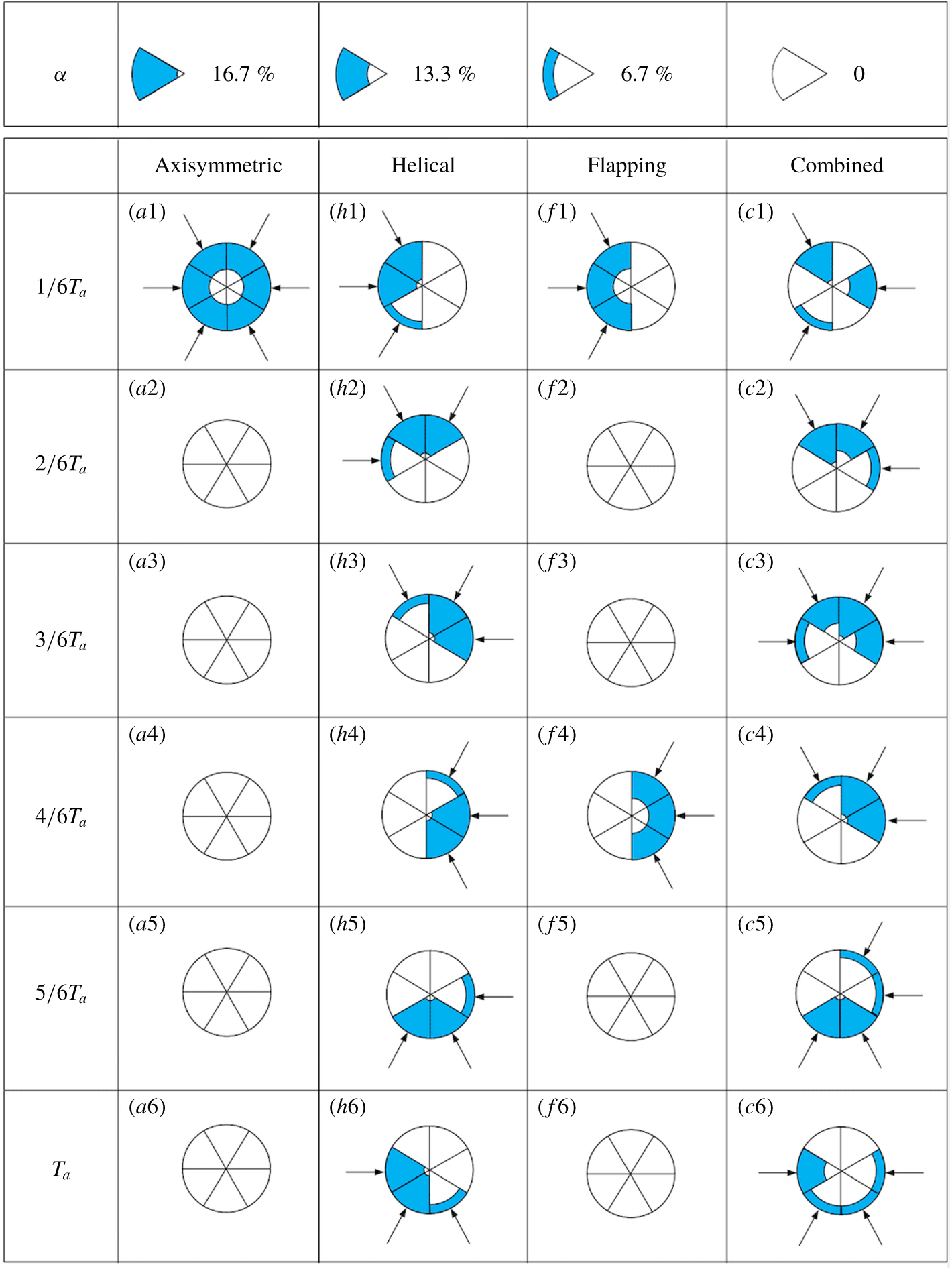
Figure 9. Actuation associated with the best individuals of generation $n=1,2,5$ and $11$ of figure 8. From top to bottom: six instances associated with $\unicode[STIX]{x1D719}=T_{a}/6,2T_{a}/6,3T_{a}/6,\ldots ,T_{a}$ in one excitation period. Each of the six sectors of the circles corresponds to one minijet.

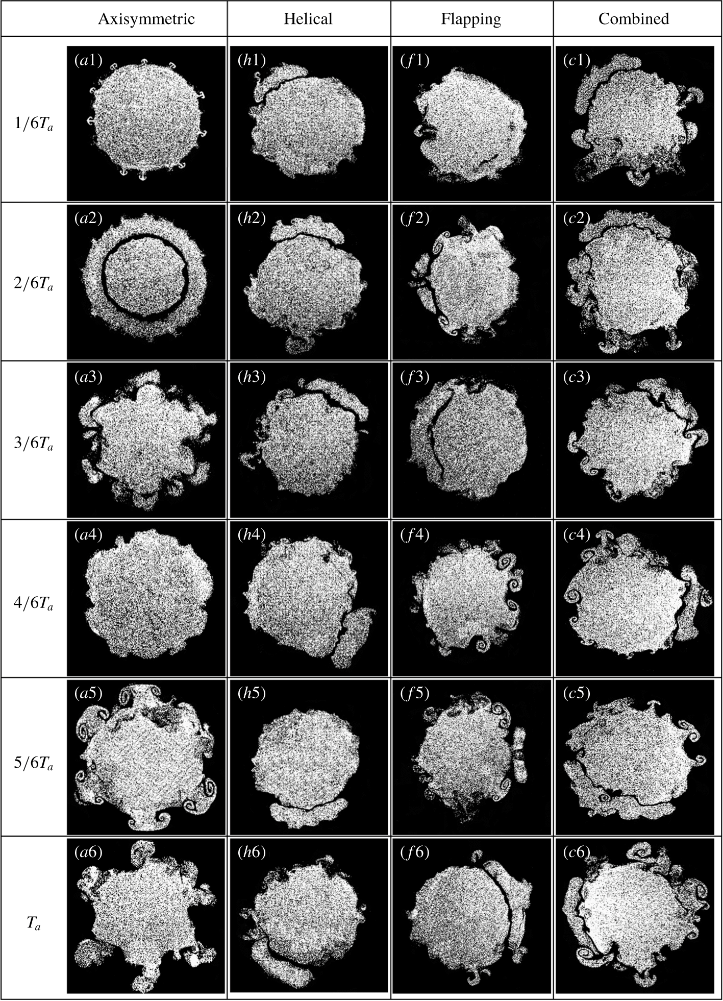
Figure 10. Sequential photographs of the cross-sectional flow structure captured at $x^{\star }=0.25$ . From top to bottom: six instances at $t_{i}=iT_{a}/6$ ( $i=1,2,\ldots ,6$ ) in one actuation period $T_{a}\,(=1/f_{a})$ .

Figure 11. Flow visualization of ( $u$ ) unforced jet, ( $a$ ) axisymmetric, ( $h$ ) helical, ( $f$ ) flapping and ( $c$ ) combined forcings from figure 8, respectively. White ellipses and crooked arrows indicate vortex rings and their rotation, respectively, and yellow arrows highlight the jet column oscillation.

5.3 Representative control laws and flow responses

The control mechanisms may be elucidated from the analysis of the spatio-temporal actuations, shown in figure 9, extracted from the control laws of $n=1$ , 2, 5 and 11. Each circular pie corresponds to one sixth of the excitation period, while its six sectors represent the six minijets. The arrow indicates that the minijet is on and the radial depth of the blue area is proportional to the duration when the minijet is injecting. The spatio-temporal actuation is found to be internally consistent with the cross-sectional and streamwise flow structure shown in figures 10 and 11. Axisymmetric forcing (figure 9 a1–a6) is characterized by simultaneous blowing of all minijets and a small $\unicode[STIX]{x1D6FC}$ of 13.3 %. As a result, the cross-sectional flow structure (figure 10 a1–a6) is axisymmetric, and the ring vortex is evident. Yang & Zhou (Reference Yang and Zhou2016) discussed in detail the distortion, formation of longitudinal structures and generation of mushroom-like structures in the braid region between ring vortices, and presented a scenario on how the interactions between the longitudinal structures, mushroom-like structures and ring vortices enhance entrainment and mixing. The six synchronized minijet excitations greatly strengthen the ring vortices, as shown in figure 11(a) (cf. figure 11 $u$ ). For helical forcing (figure 9 h1–h6), two or three minijets are blowing simultaneously at any instant, with $\unicode[STIX]{x1D6FC}$ reaching 40 %. These blowing actions rotate clockwise from ( $h1$ ) to ( $h6$ ). The greatly increased $\unicode[STIX]{x1D6FC}$ , probably required for the generation of helical motion, may act to inhibit the occurrence of mushroom-like structures (Perumal & Zhou Reference Perumal and Zhou2018), which are absent in figure 10(h1–h6). The jet (figure 11 h) exhibits more spread than axisymmetric forcing (figure 11 a). In case of flapping forcing (figure 9 f1–f6), three adjacent minijets are blowing simultaneously at one instant with $\unicode[STIX]{x1D6FC}=13.3\,\%$ and are switched to the other three after a phase shift of $\unicode[STIX]{x03C0}$ , thus creating the asymmetric flapping jet column (figures 10 f1–f6, 11 f1–f2). The actuation configuration of the rightmost column $(n=11)$ in figure 9 is complex. Firstly, the number of simultaneously injecting minijets can be 1, 2, 3 or 4, mostly adjacent to each other. Secondly, the injecting minijets tend to rotate clockwise. The resulting effect is to produce both helical and flapping motions (figures 10 c1–c6, 11 c). For convenience, hereinafter we refer to this forcing as the combined mode. Thirdly, $\unicode[STIX]{x1D6FC}$ varies from one blowing minijet to another, from about 6.7 % to 53 %. The effect could be twofold. On one hand, the varying duty cycles of the blowing minijets may yield a resultant blowing force not going through the jet centreline (figure 9 c1–c6). This may produce a precession effect, causing additional jet column oscillation (Wong, Nathan & O’Doherty Reference Wong, Nathan and O’Doherty2004). On the other hand, whilst a small $\unicode[STIX]{x1D6FC}$ facilitates the generation of mushroom-like structures (figure 10 c1–c6), a large value enhances the strength of the flapping motion (figure 11 c), as noted by Perumal & Zhou (Reference Perumal and Zhou2018). All the features, confirmed by more detailed analysis in § 6, act to promote mixing, consistent with the observed minimum $J$ (figure 8). The generation of such a sophisticated control mode, along with the generation of a complex turbulent flow structure, would have been extremely challenging for conventional control techniques, be it open- or closed-loop and model-based or model-free approaches.

5.4 Control landscape: cartographing all actuation laws

Proximity maps (§ 4.3) provide a very revealing illustration of the evolution process of the control laws. The underlying metric between two control laws $\boldsymbol{b}$ and $\boldsymbol{b}^{\prime }$ is given by $D_{ij}$ (4.4). Figure 12 presents the proximity map of the control laws in a two-dimensional plane such that this metric is optimally preserved. This plane is spanned by the feature coordinates $\unicode[STIX]{x1D6FE}_{1}$ and $\unicode[STIX]{x1D6FE}_{2}$ (§ 4.3), which are derived from a mathematical optimization process. The details of deriving $\unicode[STIX]{x1D6FE}_{1}$ and $\unicode[STIX]{x1D6FE}_{2}$ from individual generations are given in Cox & Cox (Reference Cox and Cox2000). Physically, the distance between two points, which are given in terms of ( $\unicode[STIX]{x1D6FE}_{1}$ , $\unicode[STIX]{x1D6FE}_{2}$ ), in the plane is directly linked to the extent of how closely similar to each other two control laws are.

Figure 12. Control landscape associated with generations 1, 2, 5 and 11 (400 individuals). Each symbol represents an individual control law. The colour scheme corresponds to the cost value $J$ of the control laws, e.g. (a)  $n=1$ , (b)  $n=2$ , (c)  $n=5$ , (d)  $n=11$ . The white circle of bigger size corresponds to the best individual of one generation. The elliptic contours enclose similar control laws.

The subfigures display the feature coordinates of the four discussed generations ( $n=1$ , 2, 5 and 11). Interesting observations and inferences could be made from the subfigures. For $n=1$ (figure 12 a), the points appear rather randomly distributed. The optimal solution of axisymmetric forcing, indicated by an open circle, occurs at $(\unicode[STIX]{x1D6FE}_{1},\unicode[STIX]{x1D6FE}_{2})=(-0.04,0.54)$ , where $\unicode[STIX]{x1D6FE}_{2}$ is the largest of all points. At $n=2$ (figure 12 b), these points appear forming three separated regions numbered 1 through 3, as enclosed by the elliptic contours, where most of the control laws fall in. The optimal solution that appears in region 2 and corresponds to helical forcing now occurs at $(\unicode[STIX]{x1D6FE}_{1},\unicode[STIX]{x1D6FE}_{2})=(0.39,-0.01)$ , where $\unicode[STIX]{x1D6FE}_{1}$ is the largest of all points. At $n=5$ , the individual points tend to populate along discrete curves (figure 12 c), which is a commonly observed phenomenon of the AI control, e.g. Li et al. (Reference Li, Noack, Cordier, Borée, Kaiser and Harambat2017) and Wu et al. (Reference Wu, Fan, Zhou, Li and Noack2018a ). The optimal solution now takes place at $(\unicode[STIX]{x1D6FE}_{1},\unicode[STIX]{x1D6FE}_{2})=(0.49,-0.01)$ , where $\unicode[STIX]{x1D6FE}_{1}$ is again the largest of all, within region 3, and corresponds to flapping forcing. It has been confirmed that most of the data points within regions 1, 2 and 3 correspond to axisymmetric, helical, and flapping forcings, respectively. By $n=11$ (figure 12 d), the optimal solution occurs at $(\unicode[STIX]{x1D6FE}_{1},\unicode[STIX]{x1D6FE}_{2})=(0.31,0.17)$ within region 2, corresponding to the combined mode. It is noteworthy that those points in this region now correspond to either helical or combined forcing; this very fact may suggest that the so-called combined forcing may have been developed from and more closely related to helical forcing. Interestingly, region 1, where axisymmetric forcing takes place, contracts to a single point, while region 2 or 3 is reduced to a curve.

The cost $J$ associated with each point is colour coded from red $(J=0)$ to pink $(J=1)$ , as indicated by the colour bar. The cost values within each coloured area are interpolated from the 100 individuals in each generation. The control landscape at $n=1$ displays quite a few minima, as indicated by the green coloured areas, in the feature plane (figure 12 a), suggesting the complexity of the learning task in the early stage, internally consistent with the rather random distribution of the points. The landscape becomes simpler towards the rightmost boundary of the generation. As $n$ increases, the individuals tend to line up on the ridge-curves marking the cost valleys.

Figure 13. Actuation associated with control laws $A{-}F$ , extracted from figure 12(a). The symbols are as in figure 9.

The feature coordinates have technically no a priori meaning. However, an approximate physical meaning of $\unicode[STIX]{x1D6FE}_{1}$ and $\unicode[STIX]{x1D6FE}_{2}$ may be inferred from the careful analysis of the control laws. The coordinate $\unicode[STIX]{x1D6FE}_{1}$ is correlated with the degree of asymmetric forcing, while $\unicode[STIX]{x1D6FE}_{2}$ is linked to the number of simultaneously injecting minijets. Consider six arbitrarily chosen control laws $A{-}F$ in the first generation (figure 12 a). Figure 13 shows the on- and off-states of the minijets corresponding to the six control laws. Evidently, the maximum number of simultaneously injecting minijets increases from one (law $A$ ) to six (law $F$ ).

6.1 Jet spread and predominant flow structures

Axisymmetric forcing at $n=1$ (figure 11 a) leads to an early disruption of the potential core and a significantly improved entrainment, as suggested by the substantially reduced ‘neck’ due to ambient fluid (dark colour) brought into the jet by the greatly increased strength of vortices near the nozzle exit. The flow structure exhibits an appreciably increased lateral spread than the unforced jet (figure 11 $u$ ). The $E_{u}$ of the centreline $u$ (figure 14 a) measured at $x/D=1.0$ displays the most pronounced peaks of all at $f/f_{a}=1.0$ and its harmonics, though the peaks at higher harmonics vanish rapidly from $x/D=1.0$ to 4.0. These peaks become very sharp because of the minijet excitation. The ring vortices remain axisymmetric (figure 10 a1–a6), which is corroborated by the spectral phase $\unicode[STIX]{x1D6F7}_{12}$ , about zero over the entire range of $f/f_{a}=0{-}2.0$ , between two simultaneously measured hot-wire signals $u_{1}$ and $u_{2}$ at $x/D=1$ and $y/D=\pm 0.3$ (figure 15 a). The $\unicode[STIX]{x1D6F7}_{12}$ is calculated by $\tan ^{-1}(Q_{12}/Co_{12})$ , where $Co_{12}$ and $Q_{12}$ represent the cospectrum and quadrature spectrum of $u_{1}$ and $u_{2}$ , respectively (Zhou, Zhang & Yiu Reference Zhou, Zhang and Yiu2002).

Figure 14. Normalized streamwise power spectra of fluctuating velocity $u$ measured on the centreline in the presence of the main jet: ( $a$ ) axisymmetric, ( $h$ ) helical, ( $f$ ) flapping and ( $c$ ) combined forcings.

An even larger lateral spread is achieved for helical forcing at $n=2$ (figure 11 h) due to the rotating flow structure (figure 10 h1–h6). The $E_{u}$ measured on the centreline shows less pronounced peaks at $f/f_{a}=1.0$ and its harmonics than its counterpart for axisymmetric forcing. This is because there are only two or three injecting minijets at any instant for helical forcing (figure 9 h1–h6), which produce considerably less velocity fluctuations at the jet centre than six minijets (figures 5 and 6). Furthermore, the peaks at $f/f_{a}\geqslant 2.0$ disappear at $x/D\geqslant 1$ . The $\unicode[STIX]{x1D6F7}_{12}$ is about $\unicode[STIX]{x03C0}$ over a range of frequencies about $f/f_{a}=1.0$ (figure 15 h), as is expected based on figure 9(h1–h6).

Figure 15. Phase spectrum $\unicode[STIX]{x1D6F7}_{12}$ between two streamwise fluctuating velocity signals $u$ from hot wires measured at $x/D=1$ and $y/D$ or $z/D=\pm 0.3$ .  $S_{ta}=f_{a}D/\overline{U}_{j}$ .

At $n=5$ , the jet column wobbles right and left, as indicated by yellow arrows in figure 11(f1), in the flapping plane (the $x$ – $y$ plane) but not in the orthogonal $x$ – $z$ plane (figure 11 f2), which is symmetrical about $y=0$ . The lateral spread appears exceeding appreciably that for helical forcing, echoing the considerably improved mixing shown in figure 8. Interestingly, the peaks at $f/f_{a}=1.0$ and its harmonics in $E_{u}$ are less pronounced than their counterparts of helical forcing (figure 14). The peaks of the former decay more rapidly, completely vanishing by $x/D=4.0$ , than the latter. The observation is consistent with the perception that it is the flapping motion, not the large-scale vortices, that plays a predominant role in enhancing mixing in this case. The flapping motion of the jet is characterized by a negative correlation between the two fluctuating streamwise velocities obtained on the opposite side of the jet (Goldschmidt & Bradshaw Reference Goldschmidt and Bradshaw1973). Indeed, $\unicode[STIX]{x1D6F7}_{12}$ is about $\unicode[STIX]{x03C0}$ over a very narrow frequency band about $f/f_{a}=1.0$ in the flapping plane but zero over a rather broad range of frequencies in the non-flapping plane (figure 15 f1,f2), as observed by Yang & Zhou (Reference Yang and Zhou2016). Note that the peak at $f/f_{a}=2.0$ is larger than at $f/f_{a}=1.0$ for flapping forcing (figure 14 f). This behaviour is ascribed to the flapping motion (figure 11 f1) caused by two separate excitations with a phase shift of $\unicode[STIX]{x03C0}$ within each excitation cycle (figure 9), which are captured by the hot wire.

The combined mode is distinct from all other forcings. Firstly, its spread shown in figure 11(c) is clearly the largest of all, due to the presence of both flapping and helical motions (figures 9 c1–c6 and 10 c1–c6), internally consistent with the smallest $J$ in figure 8. Secondly, its $E_{u}$ (figure 14 c) displays a number of differences from other forcings. The peak at $f/f_{a}=1.0$ grows in amplitude from $x/D=1$ to 3, while its counterpart for the other three forcings all decay quickly. Furthermore, the peaks at the higher harmonics of $f/f_{a}=1.0$ decay little for the same range of $x/D$ , in distinct contrast to their counterparts of other forcings where these peaks retreat rapidly. Naturally, compared with the other three forcing modes, there are many peaks at the higher harmonics of $f/f_{a}=1.0$ , especially at $x/D=3$ . When manipulating the main jet using a single unsteady minijet, Perumal & Zhou (Reference Perumal and Zhou2018) made a similar observation, which was ascribed to the use of a small duty cycle. The small duty cycle occurs in every phase of the combined mode (figure 9 c1–c6). Another note is that the peak at $f/f_{a}=2.0$ is larger than at $f/f_{a}=1.0$ for $x/D=1$ and remains very pronounced downstream, similarly to the flapping forcing case (figure 14 f). Thirdly, its $\unicode[STIX]{x1D6F7}_{12}$ (figure 15 c) approaches anti-phase at $f/f_{a}=1.0$ for both orthogonal planes examined. A rather broad plateau occurs at about $f/f_{a}=1.0$ , where $\unicode[STIX]{x1D6F7}_{12}\approx -0.86\unicode[STIX]{x03C0}$ . This phase shift differs appreciably in value from flapping or helical forcing where $\unicode[STIX]{x1D6F7}_{12}\approx \unicode[STIX]{x03C0}$ , and is probably connected to the presence of the oscillating component in this mode. Note that the combined mode produces the nearly anti-phased behavior for all planes through the $x$ -axis. However, in flapping forcing, this anti-phased behavior takes place only in the flapping plane.

6.2 Momentums impinging upon the main jet and jet centre trajectory

Additional insight may be gained into the flow physics of the combined mode by examining the sum of the momentums due to individual injecting minijets impinging upon the main jet and the direction of their resultant momentum. As the averaged mass flux is the same for all minijets, the maximum actuation velocity scales roughly with the inverse of the duty cycle $\unicode[STIX]{x1D6FC}$ , as demonstrated in figure 2. As such, the maximum actuation velocity $U_{a,i}$ of the $i$ th minijet is proportional to the product of $b_{i}(t)$ and $1/\unicode[STIX]{x1D6FC}_{i}$ , viz.

where $b_{i}(t)$ is a signal generated by $K_{i}(\boldsymbol{s}(t),\boldsymbol{h}(t))$ , given in (4.1), its values 0 and 1 corresponding to the on- and off-states, respectively. The time-averaged mass flow rate is the same, 1.2 %, for every minijet. The sum of the momentums due to individual injecting minijets impinging upon the main jet is parameterized by

By definition, the time-averaged amplitude is the number of active minijets, i.e. 0 for unforced flow and $\overline{A(t)}=N=6$ for actuation, implying a total time-averaged mass-flow rate of 7.2 %. On the other hand, the resultant momentum vector of the momentums associated with individual injecting minijets is given by

where 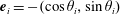$\boldsymbol{e}_{i}=-(\cos \unicode[STIX]{x1D703}_{i},\sin \unicode[STIX]{x1D703}_{i})$ is a unit vector in the direction of the $i$ th minijet located at angle $\unicode[STIX]{x1D703}_{i}$ in the $y$ – $z$ plane. The minus sign refers to an inward velocity towards the jet centre. Here $N$ is the number of injecting minijets.

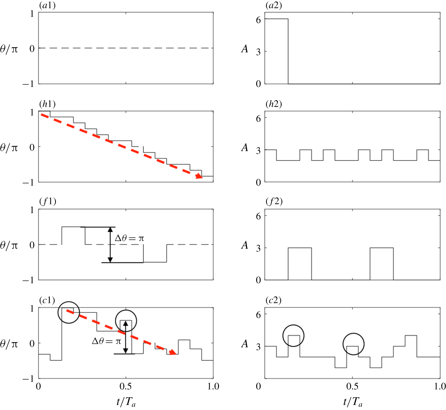
Figure 16. The angle $\unicode[STIX]{x1D703}$  (a1,h1,f1,c1) and magnitude $A(t)$ (a2,h2,f2,c2) of the effective minijet actuation vector $\boldsymbol{Q}(t)$ for the best control law of $n=1$ , 2, 5 and 11.

Figure 16 shows the variation in angle $\unicode[STIX]{x1D703}(t)$ of $\boldsymbol{Q}(t)$ , with respect to the $y$ -axis, and $A(t)$ with time $t$ over two actuation periods $T_{a}$ for the axisymmetric, helical, flapping and combined forcing modes ( $n=1$ , 2, 5 and 11). For axisymmetric forcing, $\unicode[STIX]{x1D703}(t)$ is undetermined as $\boldsymbol{Q}(t)$ vanishes identically, as 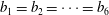$b_{1}=b_{2}=\cdots =b_{6}$ and $\sum \boldsymbol{e}_{i}=0$ (figure 9 a1). Therefore, $A(t)$ , albeit large (figure 16 a2), would not make the jet column oscillate (figure 11 a). In the case of helical forcing, $\unicode[STIX]{x1D703}$ varies essentially linearly with $t$ , as indicated by the red dashed line (figure 16 h1). The stepwise behaviour is caused by the discontinuous on–off actuation $b_{i}(t)$ . A large $A(t)$ or one half of the strength of axisymmetric forcing (figure 16 a2,f2) occurs at $t/T_{a}=0.2$ and 0.7 for flapping forcing, which correspond to a phase shift of $\unicode[STIX]{x03C0}$ (figure 16 f1). The behaviours of both $A(t)$ and $\unicode[STIX]{x1D703}(t)$ are fully consistent with our understanding of axisymmetric, helical and flapping forcings, thus providing a validation for applying $A(t)$ and $\unicode[STIX]{x1D703}(t)$ to describe the forcing on the main jet.

For the combined mode, the variations in both $A(t)$ and $\unicode[STIX]{x1D703}(t)$ with $t/T_{a}$ are more complicated. Nevertheless, a number of features can be identified. Firstly, after reaching the first maximum, as highlighted by a circle, $\unicode[STIX]{x1D703}(t)$ decreases, albeit not monotonically, over a duration of $1.3\unicode[STIX]{x03C0}$ (figure 16 c1), similarly to helical forcing, as indicated by the red arrow. This feature implies a swirling forcing on the main jet. Secondly, the maxima of A exceed those of helical forcing, suggesting a stronger swirl actuation. Thirdly, the phase shift between the second local maximum $\unicode[STIX]{x1D703}(t)$ and a local minimum $\unicode[STIX]{x1D703}(t)$ at $t/T_{a}=0.67$ is $\unicode[STIX]{x03C0}$ , as highlighted by the vertical arrow in figure 16(c1), pointing to the signature of flapping forcing. The local maximum $A$ at $t/T_{a}=0.67$ (figure 16 c2) is associated with a phase change of $\unicode[STIX]{x03C0}$ (figure 16 c1), highlighted by a circle. All the observations suggest that the combined mode is rather unique, featured by both helical and flapping motions, and further by the stronger strengths of flapping and vortical motions than other cases, thus accounting for the largest entrainment and mixing of all.

Evidently, the jet centre $\boldsymbol{r}_{c}=(y_{c},z_{c})$ responds to $\boldsymbol{Q}(t_{i})$ (6.3), and it is plausible to that assume the jet centre trajectory is correlated with $\boldsymbol{Q}(t_{i})$ . This centre can be characterized as the ‘centre of gravity’ of the streamwise velocity in a cross-stream plane of $x=\text{const.}$ :

Here, $\boldsymbol{r}=(y,z)$ represents the coordinate in the cross-stream plane. For simplicity, the $x$ -dependency of ( $y_{c},z_{c}$ ) will be dropped out hereafter. Over one excitation period with a time step $\triangle t=T/6$ , the jet centre takes six positions, i.e. 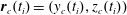 $\boldsymbol{r}_{c}(t_{i})=(y_{c}(t_{i}),z_{c}(t_{i}))$ , $t_{i}=i\triangle t$ , $i=0,1,\ldots ,5$ . We make the most simple assumption that the jet centre displacement $(\triangle y_{c},\triangle z_{c})(t_{i})=(y_{c}(t_{i+1})-y_{c}(t_{i}),z_{c}(t_{i+1})-z_{c}(t_{i}))$ over $\triangle t$ is proportional to the actuation momentum, viz.

for $i=0,\ldots ,5$ , where the proportionality constant is set to unity again for simplicity. The discrete time dynamics (6.5) can be considered to be a rough discretization of the dynamics equation $\text{d}(\boldsymbol{r}_{c})/\text{d}t=\boldsymbol{Q}$ , which describes the jet centre motion under the external momentum. Equation (6.5) represents 10 equations for 12 unknown jet centre coordinates. The remaining equations are obtained from the observation that the control law is periodic in time and the time-averaged actuation momentum vanishes based on experimental constraints, i.e. the same averaged mass flow through each minijet. Hence, the average jet centre position can be expected to vanish:

Equations (6.5) and (6.6) constitute 12 linear equations for 12 unknowns, describing the motion of the jet centre over one excitation period. The jet centre dynamics is most easily solved by starting the integration at the origin with $x_{c}(t_{0})=y_{c}(t_{0})=0$ , iteratively computing the positions at $t_{i}$ , $i=1,\ldots ,5$ with (6.5) and adding a translation consistent with a vanishing averaged jet centre (6.6).

Figure 17 presents the trajectories of the jet centre within each excitation period for the four forcings, which are calculated based on the control laws shown in figure 9 or (A 1)–(A 3) and (6.5)–(6.6). Apparently, the jet centre vanishes identically for axisymmetric forcing where $\boldsymbol{Q}(t_{i})\equiv 0$ and oscillates along the $y$ -direction between two extremes in the $x$ – $y$ plane for flapping forcing, where $\boldsymbol{Q}(t_{i})$ changes from the positive $y$ -direction at one phase to the negative at the next phase or vice versa. Helical forcing, i.e. a uniformly rotating $\boldsymbol{Q}$ vector, leads to a uniformly precessing jet and the jet centre moves along a circle around the axis of symmetry. The result conforms to previous reports. Koenig et al. (Reference Koenig, Sasaki, Cavalieri, Jordan and Gervais2016) experimentally investigated the turbulent jet under the helical mode excitation and observed a precessing jet column when the helical structures were spatially amplified in the shear layer. Zhang & Turner (Reference Zhang and Turner2016) found in a similar experiment that the jet centreline under helical excitation was offset slightly and precessed around the initial axis of the core flow. For the combined forcing, the motion of the jet centre is more complicated. Its trajectory is apparently ellipse-like, suggesting the occurrence of a precession jet. In contrast to helical forcing, the distance of the jet centre from the centre of symmetry varies, along with the separation between the centres of two consecutive phases, suggesting the speed of swirling changes with time. Furthermore, this ellipse-like path indicates an oscillating jet column, a feature of the flapping motion.

Figure 17. Jet centre trajectory ( $y_{c},z_{c}$ ) predicted from the resultant momentum vector $\boldsymbol{Q}(t_{i})$ of the momentums due to individual injecting minijets at phases $t_{i}=iT_{a}/6$ ( $i=1,2,\ldots ,6$ ).

Figure 18. Radial distributions of $\overline{U}/\overline{U}_{j}$ measured at different $x/D$ in both $x$ – $z$ and $x$ – $y$ planes for ( $u$ ) unforced jet; ( $a$ ) axisymmetric; ( $h$ ) helical; ( $f$ ) flapping, the bifurcation jet of Lee & Reynolds (Reference Lee and Reynolds1985) is included for comparison; ( $c$ ) combined.

6.3 Velocity field

The velocity field may provide us with the crucial information on the flow structure. Figure 18 presents the radial profiles of the hot wire measured $\overline{U}/\overline{U}_{j}$ at $x/D=0.05$ . A number of observations could be made. Firstly, for all controlled cases except helical forcing, the mean velocity profile displays an overshoot at the nozzle exit, as noted by Wu et al. (Reference Wu, Fan, Zhou, Li and Noack2018a ) who used a single unsteady minijet to manipulate the main jet. Andreopoulos & Rodi (Reference Andreopoulos and Rodi1984) made the same experimental observation in case of a circular jet in a cross-stream. They explained that the cross-stream fluid acted like a partial cover over the jet exit, causing the jet flow to bend around and to accelerate so that the velocity of the bent-over jet was somewhat higher than the cross-stream velocity. Secondly, the widths of the mean velocity profiles under control are larger than that of the unforced jet, indicating that the shear layer grows laterally, and the main jet becomes wider right at the nozzle exit. Thirdly, the mean velocity profiles of the axisymmetric and helical forcing at the jet exit are almost symmetrical about $y/D$ or $z/D=0$ , in general with its maximum at the centre (figure 18 a,h). The velocity profile of flapping forcing is also symmetric about $y/D$ and $z/D=0$ (figure 18 f), though displaying two peaks off the centre in the $x$ – $y$ or flapping plane and indicating the occurrence of bifurcation. As shown in figure 11(f1), two consecutive rings are locally connected, forming a zigzag flow structure, as observed in Carlos & Olivier’s (Reference Carlos and Olivier2002) numerical investigation of a bifurcating jet (their figure 4a). Furthermore, the cross-flow distributions $\overline{U}/\overline{U}_{j}$ at $x/D=3{-}5$ (figure 18 f) display two peaks in the bifurcation ( $x$ – $y$ ) plane, while those in the bisection ( $x$ – $z$ ) plane show only one peak on the centreline. Also, the jet grows slowly in width in the bisection plane. All the features are similar to Lee & Reynolds’s (Reference Lee and Reynolds1985) data where loudspeakers were used to produce a bifurcating water jet at $Re_{D}=4300$ . The present data deviate quantitatively from Lee & Reynolds (Reference Lee and Reynolds1985) as a result of distinct actuation techniques, experimental setups and $Re_{D}$ between the two investigations. Finally, the velocity profile under the combined forcing mode (figure 18 c) is distinct from others and a little tilted at the nozzle exit. Further downstream, $\overline{U}/\overline{U}_{j}$ remains asymmetrical about the jet centre but, unlike the flapping mode (figure 18 f), does not show the twin-peak distribution. Wong et al. (Reference Wong, Lanspeary, Nathan, Kelso and O’Doherty2003) produced a precession jet by issuing a jet into a cylindrical chamber with a small axisymmetric inlet at one end and an exit lip at the other. The inlet flow separates at the abrupt inlet expansion and reattaches asymmetrically to the wall of the chamber. Asymmetry of the flow within the chamber causes the reattaching flow to precess around the inner wall of the chamber, resulting in a precessing exit flow. An asymmetric and rotating pressure field is thus established so that the entire flow field, including the emerging jet, precesses (Nathan, Hill & Luxton Reference Nathan, Hill and Luxton1998). The precessing jet proves to be highly effective in increasing the near-field spreading. Interestingly, the present distributions of $\overline{U}/\overline{U}_{j}$ exhibit a similarity to their counterparts of the precession jet (please refer to figure 10 in Wong et al. (Reference Wong, Lanspeary, Nathan, Kelso and O’Doherty2003)) at the nozzle exit and downstream development.

Figure 19. Radial distributions of $u_{rms}/\overline{U}_{j}$ measured at different $x/D$ in both $x$ – $z$ and $x$ – $y$ planes for ( $u$ ) unforced jet; ( $a$ ) axisymmetric; ( $h$ ) helical; ( $f$ ) flapping; ( $c$ ) combined.

The radial distributions of $u_{rms}/\overline{U}_{j}$ (figure 19) are reasonably symmetrical about $y/D$ or $z/D=0$ under control, except under combined forcing. The $u_{rms}$ rises greatly at $x/D=0.05$ throughout the main jet, as compared to the uncontrolled jet (figure 19 $u$ ) where $u_{rms}/\overline{U}_{j}=0.3\,\%$ at $y/D=0$ and 2.5 % at $y/D\approx \pm 0.43$ due to the shear layer. The peak in the shear layer becomes very pronounced. The result suggests a turbulent jet at the nozzle exit, which is internally consistent with flow visualization data (figure 11), and the shear-layer instabilities are significantly amplified. The $u_{rms}/\overline{U}_{j}$ for axisymmetric forcing in the centre region is largest of all, due to the simultaneous injection of six minijets into the main jet, which causes a strong disturbance in the central region (figure 19 a). The $u_{rms}/\overline{U}_{j}$ distribution displays twin peaks for helical forcing (figure 19 h). This is reasonable as helical forcing may produce a hurricane-like helical motion with a centre that is more stable than the surrounding motion. The $u_{rms}/\overline{U}_{j}$ at $x/D=0.05$ under flapping forcing in the $x$ – $y$ plane is larger than in the $x$ – $z$ plane in the shear layer (figure 19 f), as observed by Hussain & Husain (Reference Hussain and Husain1989) and Zaman (Reference Zaman1996). The twin-peak behavior is evident along the $z$ -axis due to the flapping motion, but not so along the $y$ -axis. The $u_{rms}/\overline{U}_{j}$ distributions under combined forcing are asymmetrical about the centre at the jet exit (figure 19 c), and again resemble the precession jet (Mi & Nathan Reference Mi and Nathan2005). Unlike the case under flapping forcing, the $u_{rms}/\overline{U}_{j}$ profiles under combined forcing display marked twin peaks along the $y$ and $z$ axes, where the right peak is more pronounced than the left, which is probably linked to the helical motion. Furthermore, the $u_{rms}/\overline{U}_{j}$ peaks at $x/D=3$ are substantially higher along the $y$ -axis than along the $z$ -axis, which remains discernible at $x/D=5$ . All the features have been observed in the precession jet. Mi & Nathan (Reference Mi and Nathan2005) investigated the streamwise development of $u_{rms}$ in a precession jet. As shown in their figure 18, the $u_{rms}$ of the precessing jet is asymmetric compared with a non-precession jet and exhibits two peaks, located tangentially ‘in front of’ and ‘behind’ the jet centre. The ‘front’ peak is more pronounced than the ‘rear’ peak. The similar behaviours between the jet under combined forcing and a precessing jet may suggest that the so-called combined forcing may have produced a precession jet. This suggestion is further corroborated by the downstream development of the centreline mean and fluctuating velocities $\overline{U}_{cl}/\overline{U}_{j}$ and $u_{cl,rms}/\overline{U}_{j}$ presented below.

Figure 20. Streamwise variations of hot-wire measured centreline mean and r.m.s. velocities: (a)  $\overline{U}_{cl}/\overline{U}_{j}$ , (b)  $u_{cl,rms}/\overline{U}_{j}$ , (c)  $\overline{U}_{j}/\overline{U}_{cl}$ .

The variations in $\overline{U}_{cl}/\overline{U}_{j}$ , $u_{cl,rms}/\overline{U}_{j}$ and $\overline{U}_{j}/\overline{U}_{cl}$ are presented in figure 20 for various forcing modes as well as the unforced jet. It is worth pointing out that our contraction nozzle is extended by a 47 mm long smooth tube of the same diameter as the nozzle exit $D$ where the minijet assembly is mounted. In spite of this difference, the unforced jet displays the well-known features. Firstly, $f_{0}D/\overline{U}_{j}$ is 0.45, falling in the expected range $0.24{-}0.64$ (e.g. Gutmark & Ho Reference Gutmark and Ho1983; Zhou et al. Reference Zhou, Du, Mi and Wang2012). Secondly, $\overline{U}_{cl}/\overline{U}_{j}$ and $\overline{U}_{j}/\overline{U}_{cl}$ (figure 20 a,c) agree both qualitatively and quantitatively with Mi & Nathan (Reference Mi and Nathan2005) ( $Re_{D}=8050$ ) and Seidel et al.’s (Reference Seidel, Pappert, New and Tsai2005) ( $Re_{D}=8800$ ) measurements. Following Todde, Spazzini & Sandberg (Reference Todde, Spazzini and Sandberg2009), we may fit the data to 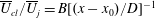$\overline{U}_{cl}/\overline{U}_{j}=B[(x-x_{0})/D]^{-1}$ , where $x_{0}$ and $B$ denote the virtual origin and decay constant, respectively. Then, $x_{0}/D=-0.49$ and $\overline{U}_{cl}/\overline{U}_{j}$ decays at a rate of $x^{-1}$ beyond $x/D=5$ , as reported by previous investigations (e.g. Mi, Nobes & Nathan Reference Mi, Nobes and Nathan2001). Thirdly, the streamwise distribution of $u_{cl,rms}$ exhibits one peak at $x/D=3.5$ and another at $x/D=7.5$ (figure 20 b). The former is connected to the breakdown of the primary ring vortices, and the latter is due to early transition to turbulence (Mi, Xu & Zhou Reference Mi, Xu and Zhou2013). Similar observations were made by Todde et al. (Reference Todde, Spazzini and Sandberg2009) (their figure 6) and by Mi et al. (Reference Mi, Xu and Zhou2013), whose data are included in figure 20(b). Departures between the present and other’s data are not unexpected in view of differences in, inter alia, experimental setup and $Re_{D}$ among the investigations. The potential core length of the unforced jet is approximately $5D$ , beyond which $\overline{U}_{cl}$ appears dropping approximately linearly. Note that $\overline{U}_{cl}/\overline{U}_{j}$ for axisymmetric forcing exceeds 1.0 given $x/D$ ${\leqslant}$ 2, higher than those of the other modes. This is due to an increase in the mass flow rate by 7.2 %. A similar observation is made by Seidel et al. (Reference Seidel, Pappert, New and Tsai2005) who observed, with 16 minijets blowing, an increase in the centreline mean velocity near the jet exit. Under all control modes, $\overline{U}_{cl}/\overline{U}_{j}$ decays rapidly right from the beginning. The minijet actuation reduces $\overline{U}_{cl}/\overline{U}_{j}$ significantly at $x/D$ ${\leqslant}8$ (figure 20 a), demonstrating the efficacy of minijet injections. This efficacy can be attributed to the earlier increase in the turbulence levels when the radial injections are present; a large turbulence level (figure 20 b) is correlated with a rapid drop in $\overline{U}_{cl}/\overline{U}_{j}$ (figure 20 a). Interestingly, the variations in $u_{cl,rms}/\overline{U}_{j}$ for helical and combined forcings are quite similar to each other, growing almost linearly first and then experiencing a small drop before fluctuating slightly around 0.15 (figure 20 b). This similarity is ascribed to the common feature of the two control modes, i.e. the swirling motion. However, it is combined forcing that maintains the rapid and linear growth further downstream, up to $x/D=3$ , and retreats little by $x/D=3.5$ . It is noted earlier in figure 14(c) that those peaks at $f/f_{a}=1$ , 2, 3, 4 and 5 in $E_{u}$ also remain pronounced up to $x/D=3$ . This coincidence suggests that the excited coherent structures account for the linear growth in $u_{cl,rms}/\overline{U}_{j}$ (figure 20 b) and the rapid decay in $\overline{U}_{cl}/\overline{U}_{j}$ (figure 20 a). In contrast, the rapid growth of $u_{cl,rms}/\overline{U}_{j}$ is only up to $x/D=2$ for helical forcing and even only up to 1 for axisymmetric and flapping forcings (figure 20 b). As such, $\overline{U}_{cl}/\overline{U}_{j}$ keeps decaying rapidly and almost linearly until $x/D=4.5$ for the combined forcing mode and remains well below other cases further downstream (figure 20 a). It is worth pointing out that the precessing jet is also characterized by a substantially faster decay than the non-precessing jet (Mi & Nathan Reference Mi and Nathan2005).

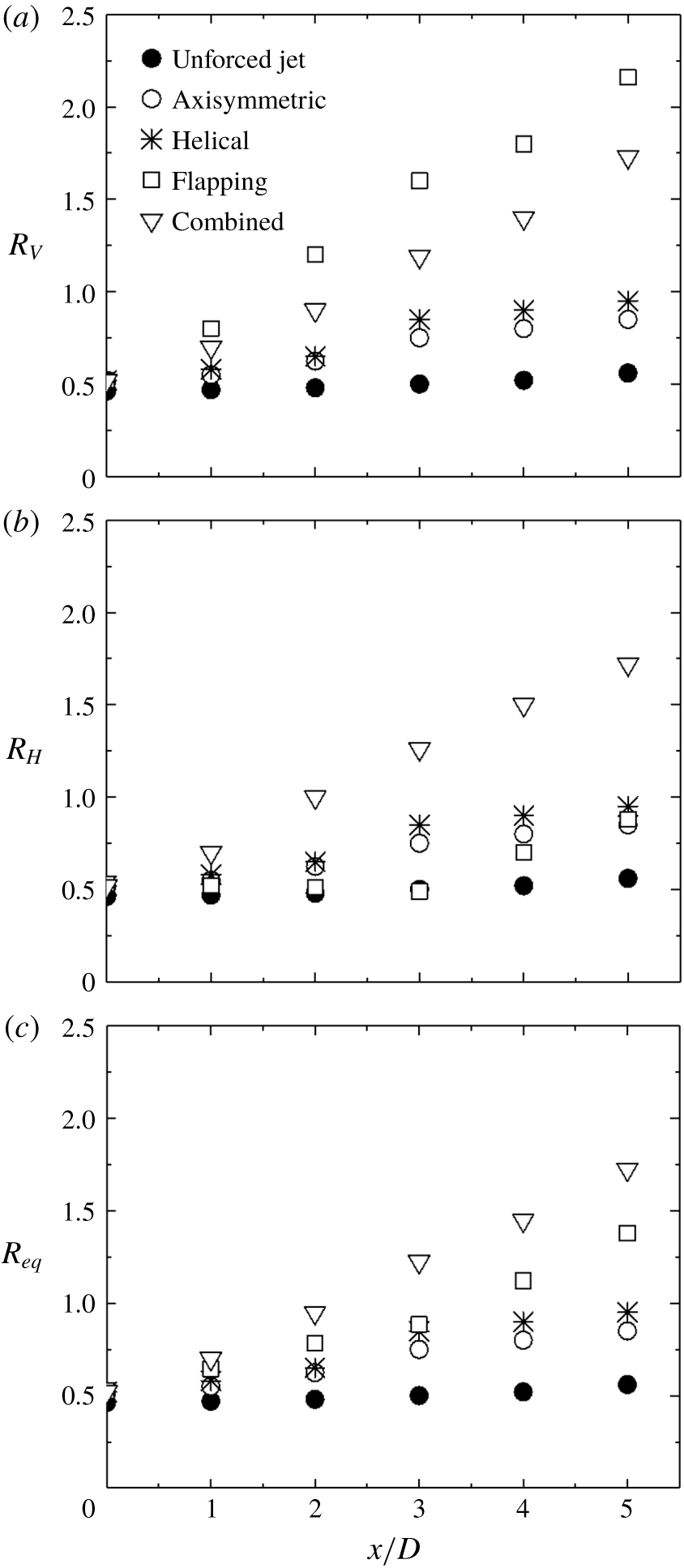
Figure 21. Mean-velocity half-widths at different $x/D$ : (a)  $R_{V}$ in the $x$ – $y$ plane, (b)  $R_{H}$ in the $x$ – $z$ plane and (c) the equivalent half-radius $R_{eq}$ .

Jet spreading rate and the overall entrainment rate may be well quantified by the downstream variation of the jet width (e.g. Zhou et al. Reference Zhou, Du, Mi and Wang2012). Following Hussain & Husain (Reference Hussain and Husain1989), we define an equivalent jet width by $R_{eq}=[R_{H}R_{V}]^{0.5}$ , where $R_{H}$ and $R_{V}$ denote the mean-velocity half-widths in the $x$ – $z$ and $x$ – $y$ planes, respectively. The half-width is defined as the distance between the jet centreline and the location at which $\overline{U}=0.5\overline{U}_{cl}$ . Figure 21 shows the downstream evolution of $R_{V}$ , $R_{H}$ and $R_{eq}$ . While changing little for the unforced jet, $R_{V}$ , $R_{H}$ and $R_{eq}$ grow appreciably in the controlled jet. Evidently, $R_{eq}$ is the largest for the combined mode, followed by flapping, helical and axisymmetric, though the latter two do not differ much. The results provide additional support for our choice of $J$ as a measure for the mixing efficacy.

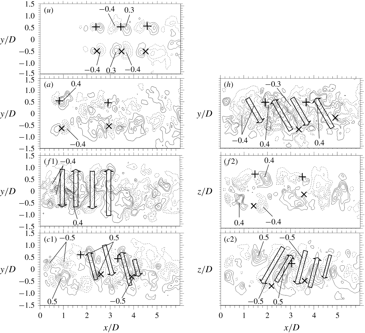
Figure 22. Isocontours of typical instantaneous velocities $V/\overline{U}_{j}$ or $W/\overline{U}_{j}$ in the $x$ – $y$ and $x$ – $z$ planes: ( $u$ ) unforced jet, ( $a$ ) axisymmetric, ( $h$ ) helical, ( $f$ ) flapping and ( $c$ ) combined forcing. Contour interval  $=$  0.1. The lowest contour level is 0.1 for all plots. Solid and broken contours represent the positive (upward motion) and the negative (downward motion), respectively. Symbols ‘ $+$ ’ and ‘ $\times$ ’ denote anti-clockwise and clockwise vortices, respectively. The arrows indicate the moving direction of the fluid slice.

To understand further the predominant flow structures under the four forcings, in figure 22 we examine typical instantaneous $V$ - or $W$ -contours, measured using PIV, in the $x$ – $y$ and $x$ – $z$ planes. In the unforced jet, the positive and negative velocity concentrations occur in pair and are mirrored by another pair, though with swapped signs, on the other side of the centreline (figure 22 $u$ ). Apparently, the two pairs of velocity concentrations are associated with the two vortical structures, as indicated by symbols ‘ $+$ ’ and ‘ $\times$ ’, of one ring vortex. Axisymmetric forcing leads to the topologically unchanged velocity contours but a significantly increased size in the velocity concentrations which now start to occur in the near proximity of the nozzle exit (figure 22 a). Under helical forcing, the vortical structures above and below the centreline are stagger-arranged and their same-signed velocity contours are connected, forming inclined strips alternately in sign (figure 22 h). Under flapping forcing (figure 22 f1), the $V$ -contours in the $x$ – $y$ plane exhibit alternate upward and downward motions which are absent in the $W$ -contours in the $x$ – $z$ plane. Some interesting observations can be made for combined forcing. Firstly, the inclined strips of velocity contours, alternately in sign, are seen in both planes (figure 22 c1,c2). Secondly, the velocity concentrations reach in general the maximum contour level of $\pm 0.5$ , greater than those associated with other forcings $(\pm 0.4)$ , indicating a stronger spread/entrainment or mixing. Thirdly, the pattern of velocity contours and their maximum strength persist considerably further downstream, reaching $x/D\approx 5$ , whilst the upward and downward motions under flapping forcing disappear at $x/D\approx 3$ , suggesting a prolonged entrainment and more thorough mixing. The observation is again internally consistent with the rapid drop until $x/D\approx 4.5$ in the centreline mean velocity decay (figure 20 a).

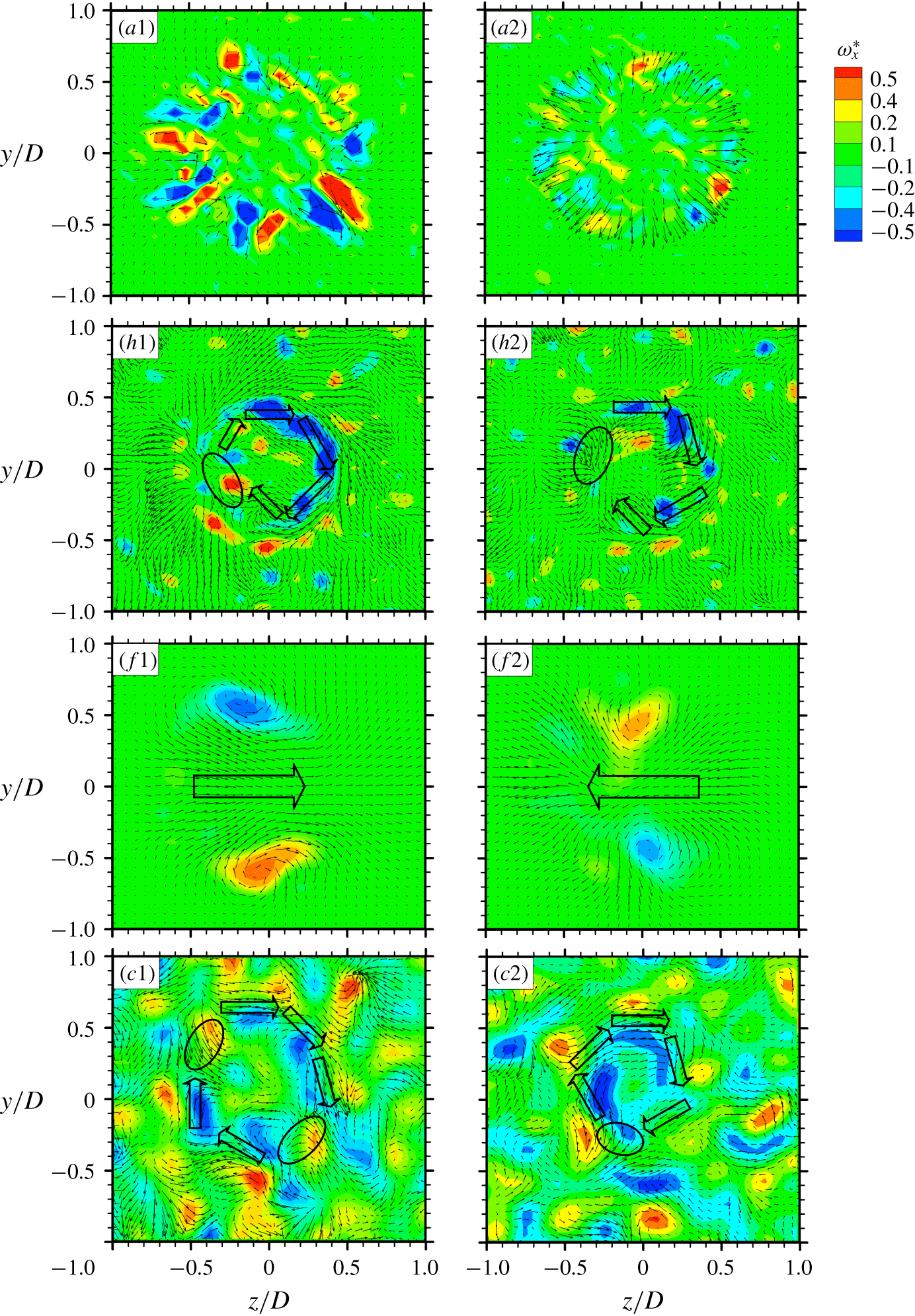
Figure 23. The typical PIV snapshots of instantaneous velocity vectors in a cross-sectional plane of ( $u$ ) unforced jet, ( $a$ ) axisymmetric, ( $h$ ) helical, ( $f$ ) flapping and ( $c$ ) combined forcings at $x/D=0.25$ . The open arrow represents the motion of the jet fluid. The elliptic contour indicates where fluid is entrained into the jet core area.

More insight may be gained into the predominant flow structures under control by examining typical instantaneous velocity vectors superimposed with the corresponding isocontours of streamwise vorticity $\unicode[STIX]{x1D714}_{x}^{\star }=\unicode[STIX]{x1D714}_{x}D/\overline{U}_{j}$ in the $y$ – $z$ plane at $x/D=0.25$ (figure 23). Under axisymmetric forcing (figure 23 a1,a2), the vectors show the inward or outward motions associated with the ring-like structures, which are axisymmetric and highly repeatable. There are six pairs of counter-rotating $\unicode[STIX]{x1D714}_{x}^{\star }$ concentrations arranged about the centre (figure 23 a), apparently generated by the six axisymmetrically placed minijets. The rotational motion under helical forcing is evident and the fluid moves inward along the circumference (figure 23 h1,h2). The core region appears rather stagnant. The phase of injecting minijets is clockwise incremented by $60^{\circ }$ (figure 9 h), producing a corkscrew type of structure (figure 10 h1–h6), as shown by Koch et al. (Reference Koch, Mungal, Reynolds and Powell1989). Figure 23(f1,f2) shows the cross-flow motion that switches from one direction at one moment to the opposite at another under flapping forcing, accompanied by one pair of counter-rotating $\unicode[STIX]{x1D714}_{x}^{\star }$ concentrations, as shown by Yang & Zhou (Reference Yang and Zhou2016). The velocity vectors in figure 23(c1,c2) exhibit the clockwise rotational motion under combined forcing. The area of rotational motion, as indicated by the arrows in figure 23(c1), is in general larger than that under helical forcing (figure 23 h1–h2). Note that ambient fluid may be entrained into the jet core area from various circumferential locations, e.g. the upper left and lower right corners, as indicated by the elliptic contours in figure 23(c1), while under helical forcing ambient fluid comes into the core area largely from only one location, as highlighted by the elliptic contours (figure 23 h1,h2). Furthermore, there are many vorticity concentrations of both signs in figure 23(c1–c2). The core area is dominated by the vorticity concentrations of negative sign, while the region surrounding the core is populated with those of both signs. This is very different from flapping forcing where there is only one pair of opposite-signed vorticity concentrations. This is also markedly different from helical forcing (figure 23 h1,h2), where the cross-sectional plane is characterized by the vorticity concentrations of a single sign. The observations reconfirm that the combined forcing mode is associated with a much better mixing and, furthermore, probably also small-scale mixing.

6.4 Insight into the three-dimensional flow structure

To gain insight into the three-dimensional flow structure, we deploy a linear stochastic estimation method to reconstruct the predominant flow structure from the PIV data, captured in the $y$ – $z$ plane at $x/D=0.25$ with a total of 200 images. This technique is introduced in detail by, for example,  Adrian & Moin (Reference Adrian and Moin1988) and is briefly described below.

Let $q(y,z,t)$ be a velocity component in the cross-plane of $x/D=0.25$ recorded at a constant sampling rate with time step $\triangle t$ , i.e.  $t_{m}=m\triangle t$ , $m=1,2,\ldots ,M$ , where $M$ denotes the total number of the PIV snapshots. Use $q^{m}(y,z)=q(y,z,t^{m})$ to denote the corresponding snapshots. The mean flow is given by

The oscillatory actuation response is the corresponding Fourier component of the fluctuation $q^{\prime }=q-\overline{q}$ . The cosine and sine contributions read as

Thus, the periodic flow response may be given by

The residual of this phase-averaged flow $\widetilde{q}$ consists of higher harmonics and an uncorrelated stochastic contribution. Note that the actuation commands $b_{i}(t)$ are the functions of the pointer ( $\cos \unicode[STIX]{x1D719}$ , $\sin \unicode[STIX]{x1D719}$ ). Hence, the temporal Fourier component optimally represents the actuation response and no flow-intrinsic phase needs to be constructed.

The isosurfaces of reconstructed $\widetilde{V}$ and $\widetilde{W}$ are presented in figure 24 for four control modes. The flow structures of axisymmetric, helical and flapping forcing modes show excellent agreement with the control laws (figure 9). Under axisymmetric forcing (figure 24 a1–a2), $\widetilde{V}$ and $\widetilde{W}$ indicate clearly that jet fluids on the two sides of the centreline move either inward or outward simultaneously (figure 24 a). Under helical forcing (figure 9 h1–h6), the helical motion is evident (figure 24 h). For flapping forcing, as indicated by the isosurfaces of $\widetilde{W}$ , one sector of fluid moves in one direction for one instant and the adjacent sectors move in the opposite direction (figure 24 f2). On the other hand, the isosurfaces of $\widetilde{V}$ is anti-symmetrical about the centreline (figure 24 f1). The observations are fully consistent with the characteristics of the flapping motion documented in, for example, Yang & Zhou (Reference Yang and Zhou2016). The results provide a validation for the presently reconstructed $\widetilde{V}$ and $\widetilde{W}$ . For the combined mode (figure 24 c), the flow structure appears much more complicated. However, the swirling motion is still discernible. Furthermore, the isosurfaces of $\widetilde{V}$ and $\widetilde{W}$ show unequivocally the occurrence of many more small parcels of fluids, suggesting a much better jet mixing than all other flow modes, which is fully consistent with the finding from figure 8 as well as figure 23(c).

Figure 24. Identification of large coherent structures by isosurfaces of phase-averaged velocity for ( $a$ ) axisymmetric ( $h$ ) helical ( $f$ ) flapping ( $c$ ) combined forcings at $x/D=0.25$ . The blue arrow indicates the direction of the jet flow.