2. Numerical methods

Three-dimensional multi-component Navier–Stokes (N–S) equations are adopted to describe the RM flow. The governing equations in conservative form are expressed as

(2.1)\begin{gather} \dfrac{\partial\rho}{\partial t} + \boldsymbol{\nabla}\boldsymbol{\cdot}(\rho{\boldsymbol{u}}) = 0, \end{gather}

(2.2)\begin{gather}\dfrac{\partial\rho\boldsymbol{u}}{\partial t} + \boldsymbol{\nabla}\boldsymbol{\cdot}(\rho\boldsymbol{u}\otimes\boldsymbol{u}+p\boldsymbol{\delta}) = \boldsymbol{\nabla}\boldsymbol{\cdot}\boldsymbol{\sigma}, \end{gather}

(2.3)\begin{gather}\dfrac{\partial\rho E}{\partial t} + \boldsymbol{\nabla}\boldsymbol{\cdot}[(\rho E + p)\boldsymbol{u}] = \boldsymbol{\nabla}\boldsymbol{\cdot}(\boldsymbol{\sigma}\boldsymbol{\cdot}\boldsymbol{u} - {\boldsymbol{q}}_c - {\boldsymbol{q}}_d), \end{gather}

(2.4)\begin{gather}\dfrac{\partial\rho Y_l}{\partial t} + \boldsymbol{\nabla}\boldsymbol{\cdot}(\rho Y_l\boldsymbol{u}) ={-}\boldsymbol{\nabla}\boldsymbol{\cdot}\boldsymbol{J}_l \quad (l = 1,\ldots,N-1), \end{gather}

where $\rho$, $\boldsymbol {u} = [u,v,w]^t$, $p$ and $E$ refer to the density, velocity vector, pressure and total energy per unit mass of the mixture, respectively, and $\boldsymbol {\delta }$ is the Kronecker delta. The equation of state is

(2.5)\begin{equation} E = \dfrac{p}{\rho(\gamma-1)}+\dfrac{1}{2}\boldsymbol{u}\boldsymbol{\cdot}\boldsymbol{u}, \end{equation}

where $\gamma$ is the specific heat ratio of the mixture and is calculated by

(2.6)\begin{equation} \gamma = \dfrac{\sum\dfrac{Y_l\gamma_l}{M_l(\gamma_l-1)}}{\sum\dfrac{Y_l}{M_l(\gamma_l-1)}}, \end{equation}

with $Y_l$, $\gamma _l$ and $M_l$ being the mass fraction, specific heat ratio and molar mass of species $l$, respectively. In this work, two species, air and ${\rm SF}_6$, are considered. In the simulations, $\gamma _1=1.4$ and $M_1=28.964\ {\rm g}\ {\rm mol}^{-1}$ are adopted for air, $\gamma _2=1.094$ and $M_2=146.055\ {\rm g}\ {\rm mol}^{-1}$ for ${\rm SF}_6$. The viscous stress tensor $\boldsymbol {\sigma }$, the conductive heat flux $\boldsymbol {q}_c$ and the interspecies enthalpy flux $\boldsymbol {q}_d$ are defined as

(2.7)\begin{gather} \boldsymbol{\sigma} = \mu[\boldsymbol{\nabla}\boldsymbol{u}+(\boldsymbol{\nabla}\boldsymbol{u})^t]- \tfrac{2}{3}\mu\boldsymbol{\nabla}\boldsymbol{\cdot}\boldsymbol{u}\boldsymbol{\delta}, \end{gather}

(2.8)\begin{gather}\boldsymbol{q}_c ={-}\kappa\boldsymbol{\nabla} T, \end{gather}

(2.9)\begin{gather}\boldsymbol{q}_d = \sum_{k=1}^{N}c_{p,k}T\boldsymbol{J}_k. \end{gather}

Here, $c_{p,k}$ is the specific heat of species $k$ at constant pressure, and the mass diffusion flux $\boldsymbol {J}_k$ is given by

(2.10)\begin{equation} \boldsymbol{J}_k ={-}\rho D_k\boldsymbol{\nabla} Y_k\quad (k=1,2), \end{equation}

for binary mixture with $D_1=D_2=D_{12}$. The viscosity $\mu$, the thermal conductivity $\kappa$ and the mass diffusion coefficient $D_{12}$ are calculated according to Tritschler et al. (Reference Tritschler, Olson, Lele, Hickel, Hu and Adams2014a).

High-fidelity simulation of compressible turbulence involving discontinuities (e.g. shock wave and material interface) and turbulent fluctuations poses a great challenge to the numerical scheme. The major difficulty lies in the simultaneous capture of discontinuities and turbulent fluctuations. On the one hand, a certain amount of numerical dissipation should be introduced into the numerical scheme to suppress spurious oscillations at discontinuities. On the other hand, minimal dissipation and dispersion (i.e. good spectral properties) are needed to accurately resolve turbulent structures covering a broad range of scales. Previous studies have shown that the existing shock-capturing schemes such as the weighted essentially non-oscillatory (WENO) scheme (Jiang & Shu Reference Jiang and Shu1996) and the WCNS scheme (Deng & Zhang Reference Deng and Zhang2000) are too dissipative to resolve small-scale turbulence. The excessive dissipation of shock-capturing schemes comes from two sources: (i) the dissipation introduced by the nonlinear mechanism and (ii) the dissipation inherent in the linear part of a nonlinear scheme. Accordingly, there are two strategies to improve the dissipation property of shock-capturing schemes. One strategy is to optimize the nonlinear weighting function, which has a significant influence on the dissipation property of the nonlinear scheme. Recently, Wong & Lele (Reference Wong and Lele2017) presented a localized dissipation WCNS with improved nonlinear weights, which has been successfully applied to RM turbulence with reshock (Wong et al. Reference Wong, Livescu and Lele2019,  Reference Wong, Baltzer, Livescu and Lele2022). Another strategy is to improve the spectral property of the corresponding linear scheme. It was found by Tam & Webb (Reference Tam and Webb1993) that the spectral property of a nonlinear scheme can be modulated by adjusting the free parameters introduced to the scheme, based on which an optimization strategy with controllable parameters was proposed (Sun et al. Reference Sun, Ren, Larricq, Zhang and Yang2011). Although the free parameters reduce the formal order of accuracy of the scheme (i.e. the rate of convergence to the exact solution with grid refinement), they can significantly improve the scheme resolution (i.e. the actual truncation error on a given mesh).

Following this idea, we have recently proposed an adaptive, nonlinear optimization strategy that considers the diversity of flow structures and the influence of nonlinearity, based on which a new type of WCNS with state-of-the-art spectral properties was developed. The optimization procedure includes: (i) two free parameters in WCNS are optimized with the approximated dispersion relation technique (Pirozzoli Reference Pirozzoli2006) that can attain the spectral properties of nonlinear WCNS; (ii) considering the nonlinear mechanism has a dramatic influence on the spectral properties, an advanced nonlinear weighting function of Wong & Lele (Reference Wong and Lele2017) is adopted and the crucial parameter, $C$, is optimized for better spectral properties; (iii) the optimized parameters are adjusted at each grid point according to the flow conditions there to realize adaptive dissipation. The optimized WCNS is extended to multi-species flows by combining the double-flux algorithm of Abgrall & Karni (Reference Abgrall and Karni2001) and is thus suitable for the simulation of RM turbulence. Note that the double-flux algorithm is not a conservative numerical method. As analysed by Abgrall & Karni (Reference Abgrall and Karni2001), there are the two main sources of conservation error for the double-flux algorithm, which have opposite effects on the solution and can nearly cancel each other out. As a result, it introduces only a little loss of conservation and thus produces a negligibly weak influence on the motions of shock and interface. In our previous work (Ding et al. Reference Ding, Si, Chen, Zhai, Lu and Luo2017,  Reference Ding, Liang, Chen, Zhai, Si and Luo2018; Feng et al. Reference Feng, Xu, Zhai and Luo2021; Li et al. Reference Li, Ding, Luo and Zou2022), the double-flux algorithm combined with the fifth-order WENO scheme has shown the capacity of reproducing the experimental results for various RM instability flows. For more details about the present numerical scheme, readers are referred to Zhou et al. (Reference Zhou, Ding, Huang and Luo2023).

As sketched in figure 1, the computational domain has a size of $2L_0 \times L_0 \times L_0$ ($L_0 = 10\ {\rm mm}$) in the $x$, $y$ and $z$ directions, which is discretized by a Cartesian mesh with $1024 \times 512 \times 512$ grid points. Two long sponge layers with a stretched mesh are set at the left and right ends of the domain along the $x$ direction, which can largely eliminate the influence of reflected waves. A periodic boundary condition is taken for the boundaries parallel to the $x$ direction. A multi-mode interface between air and ${\rm SF}_6$ at $p = 101\,325\ {\rm Pa}$ and $T = 298.15\ {\rm K}$ is set at the beginning, whose average position is at $x=0.11L_0$. A planar shock of $Ma =1.5$ is initially set at $x=-L_0/4$ in air. To ensure the shocked interface evolves at the centre of the domain, the pre-shock gases are set to move at $\Delta U = -158.38\ {\rm m}\ {\rm s}^{-1}$.

Figure 1. Schematic of the computational domain.

The initial multi-mode interface is set according to Groom & Thornber (Reference Groom and Thornber2020), which has a power spectrum

(2.11) \begin{equation} P(k)=\left\{\begin{array}{@{}ll} Ck^m, & k_{min}< k< k_{max},\\ 0, & {\rm otherwise}, \end{array} \right. \end{equation}

where $k=\sqrt {k_y^2+k_z^2}$ is the radial wavenumber. In this work, two cases with $m=0$ are simulated. One case has initial narrowband Fourier modes, namely, $k_{n} \in (24,40)$ with $k_{n} = ({L_0}/{2{\rm \pi} })k$ (called case NB). The other case has initial broadband Fourier modes, namely, $k_{n} \in (2,64)$ (called case BB). To reach the turbulent state faster, the total standard deviation of the perturbation is fixed at $\sigma = 0.5\lambda _{min}$ for both cases. In order to deposit more kinetic energy on the post-shock interface to feed the subsequent turbulence, the initial interface thickness is set to be a small value of $\lambda _{min}/4$ (Lombardini et al. Reference Lombardini, Pullin and Meiron2012).

The dissipation scale $\eta$, also known as the Kolmogorov scale, is usually considered as the smallest characteristic scale in turbulence. Thus, a criterion for direct numerical simulation (DNS) is that the grid is fine enough such that the dissipation scale is resolved. It is found in practical simulations that this criterion can be relaxed somewhat, namely, the grid size is of the order of $\eta$ rather than equal to $\eta$ (Moin & Mahesh Reference Moin and Mahesh1998). According to the finding of Moin & Mahesh (Reference Moin and Mahesh1998) that most of the dissipation in the channel flow occurs at scales greater than $15\eta$, Li et al. (Reference Li, He, Zhang and Tian2019) argued that a grid resolution of around $10\eta$ is qualified for DNS. Liu & Xiao (Reference Liu and Xiao2016) and Tritschler et al. (Reference Tritschler, Zubel, Hickel and Adams2014b) advocated the criterion of Yeung & Pope (Reference Yeung and Pope1989), i.e. the dissipation becomes extremely small beyond $k\eta =1.5$, and thus $k_{\Delta max}\eta \geqslant 1.5$ ($k_{\Delta max}={\rm \pi} /\varDelta$ with $\varDelta$ the grid size) can be used as a criterion for DNS. With these two criteria, the grid resolution of the present simulations is examined, as shown in figure 2(a) where $\eta$ is calculated by the method of Tritschler et al. (Reference Tritschler, Zubel, Hickel and Adams2014b). The results indicate that both cases satisfy the criterion of Moin & Mahesh (Reference Moin and Mahesh1998), but cannot meet the criterion of Yeung & Pope (Reference Yeung and Pope1989). Actually, the more restrictive latter criterion is more appropriate for DNS, particularly for the study of high-order statistics. It should be noted that the idea of using the Kolmogorov scale to represent the smallest scale of the flow is not justifiable, because the time-dependent RM flow is not always in a state of fully developed turbulence (Groom & Thornber Reference Groom and Thornber2019; Zhou et al. Reference Zhou, Williams, Ramaprabhu, Groom, Thornber, Hillier, Mostert, Rollin, Balachandar and Powell2021). Also, the shock-capturing scheme that involves numerical dissipation can influence the accuracy in estimating the viscous dissipation rate, and can further affect the calculated Kolmogorov scale. The present analysis shows that the grid resolution of the current simulations is close to, rather than at, the level of DNS. Note that the Schmidt number of the present flow is $Sc \approx 1$, under which the Bachelor scale is almost the same as the Kolmogorov scale. Since the N–S equations are solved with a high-resolution numerical scheme in this work, the present simulations (without an explicit subgrid-scale model) are referred to as high-fidelity N–S simulations according to Zhou et al. (Reference Zhou, Williams, Ramaprabhu, Groom, Thornber, Hillier, Mostert, Rollin, Balachandar and Powell2021). A grid sensitivity study on the turbulence statistics is given in the Appendix to show the uncertainty of the simulation results.

Figure 2. (a) Temporal evolution of the normalized Kolmogorov scale and (b) variation of the turbulence Reynolds number vs Taylor Reynolds number, averaged within the inner mixing zone, for case NB (squares) and case BB (circles).

To better characterize the flow, the evolutions of the turbulence Reynolds number ($Re_{L}$) and Taylor Reynolds number ($Re_{\lambda _T}$) are given in figure 2(b). The former is characterized by large eddies and the latter is related to small and intermediate scales. These two Reynolds numbers are calculated by (Pope Reference Pope2000)

(2.12)\begin{equation} Re_{L} = \dfrac{\left\langle K\right\rangle_{yz}^2}{\left\langle\rho\right\rangle_{yz}\left\langle\varepsilon\right\rangle_{yz} \left\langle\nu\right\rangle_{yz}}, \end{equation}

and

(2.13)\begin{equation} Re_{\lambda_T} = \dfrac{\left\langle u_r^{\prime\prime}\right\rangle _{yz}\left\langle \lambda_{T}\right\rangle _{yz}}{\left\langle \nu\right\rangle _{yz}}, \end{equation}

where $\left \langle K\right \rangle _{yz}=\sum _{k} E_{TKE}(k,x,t)$, $\varepsilon =\sum _{k} 2\left \langle \nu \right \rangle _{yz}k^2 E_{TKE}(k,x,t)$ and $\nu =\mu /\rho$ are the kinetic energy, dissipation rate and kinematic viscosity, respectively; $u_r^{\prime \prime }=({v^{\prime \prime }}^2+{w^{\prime \prime }}^2)^{1/2}$ and $\left \langle \lambda _{T}\right \rangle _{yz}=(10\left \langle \nu \right \rangle _{yz}\left \langle K\right \rangle _{yz}/\left \langle \varepsilon \right \rangle _{yz})^{1/2}$ are the radial velocity fluctuation and Taylor scale, respectively; $\varphi ^{\prime \prime }=\varphi -\left \langle \rho \varphi \right \rangle _{yz}/\left \langle \rho \right \rangle _{yz}$ is defined as the fluctuating part of the Favre average, and $\left \langle {\cdot }\right \rangle _{yz}$ refers to the spatial average in the $yz$ plane. The radial power spectrum for variable $\varphi$ is given as

(2.14)\begin{equation} E_{\varphi}(k)=\sum_{k-1/2<\lvert\boldsymbol{k}_{yz}\rvert\leqslant k+1/2}\hat{\varphi}^{{\star}}\hat{\varphi}, \end{equation}

where $\hat {\varphi }$ is the Fourier transform of $\varphi$ in the $yz$ plane, and $\hat {\varphi }^{\star }$ denotes its complex conjugate. In the present work, $\varphi =\sqrt {\rho }u_i^{\prime \prime }$ is used to calculate the spectrum of turbulent kinetic energy (TKE). As shown in figure 2(b), both cases present a similar evolution for $Re_{\lambda _T}$ in the interval ($30, 120$) and for $Re_{L}$ in the interval ($200, 7000$). The scaling for both cases is quite close to the relationship, $Re_{L} \propto Re_{\lambda _{T}}^{2}$, in HIT.

3. Characteristics of RM turbulence

The growth of the mixing width, which plays an important role in the establishment of the phenomenology for RM turbulence, is first investigated. The mixing width is calculated by

(3.1)\begin{equation} W_f=\int 4\!\left\langle\, f_1\right\rangle _{yz}\left\langle\, f_2\right\rangle _{yz} \,{\rm d}\kern 0.06em x, \end{equation}

where $f_1$ and $f_2 = 1 -f_1$ denote the volume fractions of species 1 and 2, respectively. The mixing width is normalized as $W_f/\bar {\lambda }$ according to Groom & Thornber (Reference Groom and Thornber2021). Here, $\bar {\lambda }=2{\rm \pi} /\bar {k}=L_0/\bar {k}_n$ is the average wavelength, in which $\bar {k}_n$ denotes the weighted average wavenumber and is calculated by

(3.2)\begin{equation} \bar{k}_n=\dfrac{\sqrt{\displaystyle\int\nolimits_0^{\infty}k^2p(k)\,\text{d}k}}{\sqrt{\displaystyle\int\nolimits_0^{\infty}p(k)\, \text{d}k}}=\sqrt{\dfrac{1}{3}\left(1+\dfrac{1}{R}+\dfrac{1}{R^2}\right)}k_{max}, \end{equation}

where $R=k_{max}/k_{min}$. Time is normalized by $\bar {\lambda }/\dot {W}_0$, where $\dot {W}_0$ is the initial growth rate that is estimated by

(3.3)\begin{gather} \dot{W}_0=0.564\bar{k}A^+\sigma_0^+\Delta U, \end{gather}

(3.4)\begin{gather}\sigma_0^+ = \left(1-\frac{\Delta U}{U_s}\right)\sigma_0, \end{gather}

where $A^+$ and $\sigma ^+$ are the post-shock Atwood number and post-shock standard deviation of the perturbation, respectively, and $U_s$ is the velocity of the initial shock.

As shown in figure 3(a), good agreement between the numerical result and the nonlinearly fitted curve is obtained, which indicates an evident $(\tau -\tau _0)^{\theta }$ ($\tau _0$ is a virtual time origin) growth behaviour in the self-similar stage for each case. The curve fit is performed over the range $\tau \geqslant 5$ for both cases, and the fitted value of $\theta$ is $0.211$ ($0.333$) for case NB (case BB). Recently, under the small Atwood number Boussinesq approximation, Soulard et al. (Reference Soulard, Guillois, Griffond, Sabelnikov and Simoëns2018) deduced a relationship between the self-similar growth rate of the RM mixing layer and the infrared slope ($s_0$) of the post-shock velocity spectrum, $\theta = 2/(s_0+4)$, where $s_0=m^{\prime }+1$ with $m^{\prime }$ being the infrared exponent of the interface perturbation spectrum. According to Elbaz & Shvarts (Reference Elbaz and Shvarts2018) and Soulard et al. (Reference Soulard, Guillois, Griffond, Sabelnikov and Simoëns2018), the evolution of the mixing width is influenced by both the behaviour of the large scale itself and the nonlinear backscatter of small scales to the large scale. For case NB with a high-wavenumber narrowband perturbation spectrum, the latter factor dominates the evolution of the mixing width. Based on this cognition, $\theta$ is predicted to be $1/3$ by Elbaz & Shvarts (Reference Elbaz and Shvarts2018) and $1/4$ by Soulard et al. (Reference Soulard, Guillois, Griffond, Sabelnikov and Simoëns2018). For case BB with initial large-scale perturbations $\theta$ is expected to be $2/5$ from the prediction of Soulard et al. (Reference Soulard, Guillois, Griffond, Sabelnikov and Simoëns2018). Figure 3(b) gives the variation of the instantaneous growth rate exponent from simulation, which is calculated as $\theta =1/(1+\beta )$ with $\beta =-W\ddot {W}/\dot {W}^2$ (Oggian et al. Reference Oggian, Drikakis, Youngs and Williams2015). According to Oggian et al. (Reference Oggian, Drikakis, Youngs and Williams2015) and Groom & Thornber (Reference Groom and Thornber2021), the fluctuations in $\theta$ are mainly ascribed to the numerical derivative (especially the second derivative) that magnifies the noise of the data. We state that this type of fluctuation does not hinder the judgment of the overall variation trend of $\theta$. As we can see, the instantaneous value of $\theta$ is generally consistent with the fitted one. Moreover, it gradually approaches the prediction of Soulard et al. (Reference Soulard, Guillois, Griffond, Sabelnikov and Simoëns2018) for each case. It is also seen that $\theta$ presents a trend of increasing to a higher value at the end time of the simulation.

Figure 3. Temporal evolution of (a) the mixing width $W$ and (b) the instantaneous growth rate exponent $\theta$ for case NB (squares) and case BB (circles). Lines in (a) represent the fit of $a(\tau -\tau _0)^\theta$, where $\tau _0$ is a virtual time origin.

Also, there are other definitions of the mixing width, such as the mass-fraction-based one, $W_{Y}$, which is calculated by replacing the volume fraction $f$ with mass fraction $Y$ in (3.1). The relationship between the two kinds of mixing width is investigated. Suggested by Boffetta et al. (Reference Boffetta, Mazzino, Musacchio and Vozella2010), the integral length scale that represents the dynamical characteristic scale of large eddies is also investigated. Here, the integral length scale is calculated by (Pope Reference Pope2000)

(3.5)\begin{equation} \varLambda = \frac{3{\rm \pi}}{4}\frac{\displaystyle\int\nolimits_0^{\infty}E(k)/k\,{\rm d}k}{ \displaystyle\int\nolimits_0^{\infty}E(k)\,{\rm d}k}, \end{equation}

and then averaged in the inner mixing zone (IMZ) which is defined by $4Y(1-Y)\geqslant 0.9$ (Tritschler et al. Reference Tritschler, Olson, Lele, Hickel, Hu and Adams2014a). Figure 4 shows the variations of $W_{Y}$ and $\varLambda$ vs $W_{f}$. It is found that these scales are linearly related in the self-similar state. Performing a linear fit, the correlations of $W_Y \propto 1.01W_f$ ($W_Y \propto 1.17W_f$) and $\varLambda \propto 0.42W_f$ ($\varLambda \propto 0.36W_f$) for case NB (case BB) are obtained. This indicates that these typical large characteristic scales have similar scaling behaviour, which is favourable for the development of a phenomenological theory (Chertkov Reference Chertkov2003).

Figure 4. The variations of the mass-fraction-based mixing width $W_Y$ and the integral length scale $\varLambda$ vs the volume-fraction-based mixing width $W_f$. The symbols are the same as those in figure 3.

Before moving to the discussion of the structure function, we examine the evolution of the IMZ-averaged TKE spectra calculated by (2.14) for cases NB and BB, as shown in figure 5. Since the dynamics of RM turbulence originates from the energy deposited by the initial shock wave, the initial perturbation spectrum at the interface determines the range of the energy scale (mainly in the direction of shock wave propagation). The Kolmogorov spectrum can only appear in the scale range below the initial maximum scale, and the spectrum above the initial maximum scale is mainly ascribed to the inverse transfer of energy from small to large scales.

Figure 5. The TKE spectra (a,b), TKX spectra (c,d) and TKYZ spectra (e,f) of case NB (a,c,e) and case BB (b,d,f) at several times.

For case NB with a high-wavenumber narrowband perturbation spectrum, there exists a visible $k^{-3/2}$ spectrum at the early stage. As time proceeds, the spectral peak shifts to lower wavenumbers and the $k^{-3/2}$ spectrum is gradually swallowed by a shallower spectrum, similar to the results of Tritschler et al. (Reference Tritschler, Olson, Lele, Hickel, Hu and Adams2014a,Reference Tritschler, Zubel, Hickel and Adamsb) and Grinstein et al. (Reference Grinstein, Gowardhan and Wachtor2011). At the late stage, the range of the $k^{-3/2}$ spectrum becomes very narrow. We further examine the TKX (the $x$ components of TKE) and TKYZ (the $y$ and $z$ components of TKE) spectra for case NB. Results show that the early spectral distributions in the $x$, $y$ and $z$ directions present significant differences. The $x$-component energy is higher than that of the $y$ and $z$ components, revealing the anisotropic characteristics of RM turbulence. The $k^{-3/2}$ spectrum of TKE at the early stage is mainly contributed by the $x$-component fluctuations. The $yz$-component only presents a narrower $k^{-3/2}$ spectrum at higher wavenumbers, which may be due to the energy transfer from the $x$ direction to the $yz$-directions. For case BB with a broadband perturbation spectrum, at $\tau =1.59$, the TKE, TKX and TKYZ show the $k^{(m+2)/2}$ spectrum ($m=0$ in this work) suggested by Youngs (Reference Youngs2004), which is consistent with the results of Groom & Thornber (Reference Groom and Thornber2020). Later, a $k^{-3/2}$ spectrum appears for TKX, while TKYZ holds this spectrum in a narrower range at high wavenumbers. As time proceeds, the $x$-component gradually approaches the $yz$-component and the spectrum in the lower-wavenumber range becomes progressively shallower.

Figure 6 shows the spectra of $Y_{\text {SF}_6}$ for both cases. As we can see, the mass fraction spectrum has a wider $k^{-3/2}$ spectral range than the TKE spectrum. This is more obvious in case BB.

Figure 6. The radial spectra of mass fraction $Y_{\text {SF}_6}$ for case NB (a) and case BB (b) at several times. The line styles represent the same times as in figure 5.

Then, we consider the structure function of the longitudinal velocity, defined as $S^L_p(r,t) \equiv \left \langle \lvert \delta _r u/u^{\prime \prime }_{rms}\rvert ^p\right \rangle$, where $\delta _r u=[\boldsymbol {u}(\boldsymbol {x}+\boldsymbol {r},t)-\boldsymbol {u}(\boldsymbol {x},t)] \boldsymbol {\cdot } \hat {\boldsymbol {r}}$ with $\hat {\boldsymbol {r}}=\boldsymbol {r}/\lvert \boldsymbol{r} \rvert$ and $u^{\prime \prime }_{rms}$ being the root-mean-square of the velocity fluctuation. Also, the scalar structure function in terms of the mass fraction of heavy fluid is examined, which is defined as $S_p^{Y_{{\rm SF}_6}}(r,t) \equiv \left \langle \lvert \delta _r Y_{\rm SF_6} \rvert ^p\right \rangle$ where $\delta _r Y_{{\rm SF}_6}=Y_{{\rm SF}_6}(\boldsymbol {x}+\boldsymbol {r},t) - Y_{{\rm SF}_6}(\boldsymbol {x},t)$. In this work, both velocity and scalar structure functions are calculated in a statistically homogeneous direction (e.g. the $y$ direction) and then spatially averaged in the IMZ. Thus, $\boldsymbol {r}$ and $\left \langle {\cdot }\right \rangle$ in the above formulae can be replaced by $\boldsymbol {r_y}=(0,r_y,0)$ and $\left \langle {\cdot }\right \rangle _{IMZ}$, respectively. We note that, whether $\boldsymbol {r_z}=(0,0,r_z)$ or is averaged in the central plane of the mixing layer (Walchli & Thornber Reference Walchli and Thornber2017), the main results are almost the same. Due to the limited computational resource, the turbulence simulated usually involves only a narrow inertial range, which increases the measurement uncertainty of the scaling exponent. To overcome this difficulty, an extended self-similarity (ESS) method (Benzi et al. Reference Benzi, Ciliberto, Baudet and Chavarria1995) that investigates the scaling of the $n$th-order structure function against the $m$th-order, i.e. $S_n(r) \sim S_m(r)^{\beta _{(n,m)}}$, is adopted to obtain an accurate relative scaling exponent, $\beta _{(n,m)}=\zeta _n/\zeta _m$. As suggested by Boffetta et al. 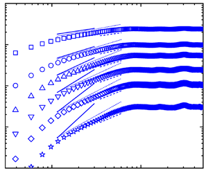(Reference Boffetta, Mazzino, Musacchio and Vozella2010), here, the reference exponents for the structure functions of velocity and mass fraction take the forms $\zeta ^{L}_3$ and $\zeta ^{Y_{\rm SF_6}}_2$, respectively. Variations of the first- to sixth-order structure functions vs the reference one at a fixed time using a log–log scale for cases BB and NB are plotted in figure 7. As we can see, all orders of structure functions show a linear relationship with the reference one, which indicates the existence of ESS scaling. The slope of each-order structure function against the reference one corresponds to the relative scaling exponent. The values of $\beta ^L_{(p,3)}$ and $\beta ^{Y_{\rm SF_6}}_{(p,2)}$ can be obtained via least-square fits. As shown in figure 7, the fitted lines agree well with the simulation results. It is also found that the scaling range becomes narrower as $p$ increases. Note that the fittings are carried out with an appropriate range of data points, which ensures that the distributions of the compensated structure functions against the reference one are as close as possible to the horizontal line (Pan & Scannapieco Reference Pan and Scannapieco2011), as shown in the insets of figure 7.

Figure 7. The ESS spatial scaling of (a,c) the longitudinal velocity structure function $S^L_p$ and (b,d) the scalar structure function $S_p^{Y_{{\rm SF}_6}}$ with $p=1$ (squares), 2 (circles), 3 (up triangles), 4 (down triangles), 5 (diamonds), 6 (stars). Data are from (a,b) case NB at $\tau =43.94$ and (c,d) case BB at $\tau =59.24$. The insets are the corresponding compensated structure functions. Note that each plot of $S_p^L$ is offset by 0.65, 0.35, 0.15 and 0.05 for $p=3{-}6$, respectively. The plot of the compensated structure function in the inset of (d) is offset by $p$ for $p=2\unicode{x2013}6$, respectively.

The relative scaling exponents obtained via least-square fits are given in figure 8, where the Kolmogorov–Obukhov–Corrsin (KOC) predictions are also given for comparison. Figure 8(a) also gives the relative scaling exponents in HIT with scalar injection by the Gaussian random source (Gotoh et al. Reference Gotoh, Watanabe and Suzuki2011) and in RT turbulence at small Atwood number (Boffetta et al. Reference Boffetta, Mazzino, Musacchio and Vozella2010) for comparison. It is found that the relative exponents for RT turbulence and HIT are nearly identical to the present results of RM turbulence up to fourth order. At higher orders, there exists a visible discrepancy among them. The phenomenological theory fails to give an accurate prediction for $p>3$, which indicates the existence of intermittency in the velocity field. This is a consequence of the breakdown of scale independence (an underlying assumption for phenomenological theory) caused by the fluctuations of energy and scalar dissipation rate. The relative scaling exponents for different types of turbulence are consistent with the prediction of the She–Leveque (SL) model (She & Leveque Reference She and Leveque1994) that considers the influence of intermittency. The present results give strong evidence that there exists intermittency for RM turbulence as with RT turbulence and HIT. Figure 8(b) gives a comparison of the scalar scaling exponent among the RM turbulence, RT turbulence, two types of HIT and the KOC prediction. Visible differences between the results of the two cases is observed. As we know, the 4/5 law by Kolmogorov (Reference Kolmogorov1941a) is related to the third-order structure function of the velocity, and the corresponding law by Obukhov (Reference Obukhov1949) and Corrsin (Reference Corrsin1951) is related to the second-order structure function passive scalar. This is the reason for the choices of $\beta _{(p,3)}^L$ for the velocity and $\beta _{(p,2)}^C$ for the scalar (Boffetta et al. Reference Boffetta, Mazzino, Musacchio and Vozella2010) here. It is found that the scalar scaling exponents for case NB nearly coincide with those of HIT with scalar injection through a uniform gradient, whereas the exponents for case BB coincide with those of RT turbulence and HIT with random Gaussian source. We note that the fluctuations in case NB are only generated by small-scale perturbations, while those in case BB are also related to the cascade of large-scale perturbations. The previous study of Gotoh et al. (Reference Gotoh, Watanabe and Suzuki2011) on HIT showed that the passive scalar fluctuations are excited at all scales for the case with scalar injection by velocity excitation through a uniform gradient, but are mainly excited through the scale cascade for the case with scalar injection by a Gaussian random source at large scales. This can be used to speculate on the origin of the difference in passive scalar statistics at small scales under different initial conditions.

Figure 8. Relative scaling exponents for (a) longitudinal velocity structure functions $\beta ^L_{(p,3)}$ and (b) scalar structure functions $\beta ^{C}_{(p,2)}$. Data shown are from case NB (red filled circles), case BB (blue filled stars), DNS of RT turbulence with end time $Re_{\lambda }=196$ in Boffetta et al. (Reference Boffetta, Mazzino, Musacchio and Vozella2010) (black open circles), DNS of HIT with scalar injection by isotropic Gaussian random source at $Re_{\lambda }=688$ (black up triangles) and by uniform gradient at $Re_{\lambda }=586$ (black down triangles) in Gotoh, Watanabe & Suzuki (Reference Gotoh, Watanabe and Suzuki2011) and DNS of HIT with scalar injection by an isotropic random Gaussian source at $Re_{\lambda }=427$ in Watanabe & Gotoh (Reference Watanabe and Gotoh2004) (black squares). Solid lines in both panels represent the KOC phenomenological predictions. The dotted line indicates the prediction of the She–Leveque model (She & Leveque Reference She and Leveque1994).

All simulation results deviate from the model prediction for $p>2$, which is ascribed to the presence of intermittency. To support this statement, we undertake a hierarchical symmetry analysis that was originally proposed by She & Leveque (Reference She and Leveque1994) and then rewritten by She et al. (Reference She, Ren, Lewis and Swinney2001):

(3.6)\begin{equation} \dfrac{F_{p+1}(r)}{F_2(r)}=\dfrac{A_p}{A_1}\left(\dfrac{F_p(r)}{F_1(r)}\right)^{\hat{\beta}}, \end{equation}

where $F_p (r)=S_{p+1}(r)/S_p(r)$ is the hierarchy, $A_p$ is a parameter independent of $r$ and $\hat {\beta }\leqslant 1$ reflects the degree of intermittency (lower value of $\hat {\beta }$ corresponds to stronger intermittency). It is noted that $\hat {\beta }=1$ corresponds to the Kolmogorov scenario without intermittency, and $\hat {\beta }=(2/3)^{1/3}\approx 0.874$ in the SL model for isotropic turbulence. As shown in figure 9, the scaling of hierarchical symmetry with $\hat {\beta }<1$ is obtained for the velocity and scalar in cases NB and case BB, which is consistent with the departures of the scaling exponents of the two cases from the KOC formulation. The value of $\hat {\beta }\approx 0.76$ for velocity is lower than the value used in the SL model, which explains the departures of the high-order scaling exponents of both cases from the prediction of the SL model. The lower value of $\hat {\beta }$ for scalar (${\approx }0.63$) than that of velocity (${\approx }0.76$) also corresponds to the stronger intermittency of the scalar than the velocity. The present analysis indicates that intermittency is closely related to the symmetry breaking between scales. As we know, the symmetry breaking is related to a variety of factors such as the flow type, initial conditions, Mach number and so on. This may be the reason why cases BB and NB with different initial perturbation spectra present different degrees of intermittency.

Figure 9. Scaling of hierarchical symmetry of (a) velocity and (b) scalar for case NB (red) and case BB (blue) with $p=2$ (circles), $3$ (up triangles) and $4$ (down triangles).

From the present results, two claims can be made for RM turbulence. First, as we know, the only difference between case NB and case BB is the initial perturbation spectrum. Since these two cases present different behaviours of small-scale statistics, it is reasonable to speculate that larges scales in case BB can influence the statistics of small scales. Especially, it is found that the difference in anomalous scaling exponents between case NB and case BB is larger for the scalar structure function than the velocity structure function. This indicates that the statistics of small-scale scalar fluctuations suffer a larger influence of large scales than the velocity fluctuation. Second, the scalar field exhibits a greater degree of intermittency than the velocity field under the current Mach number. Particularly, the deviation of the RM turbulence from other types of turbulence for both $\beta ^{L}_p$ and $\beta ^{C}_p$ highlights the unique characteristic of RM turbulence, and thus a specific phenomenological theory for RM turbulence is desired.

4. Phenomenological model and validation

A key idea of the present phenomenological theory for RM turbulence is to introduce an external agent inspired by Zhou (Reference Zhou2001). With (1.1) and the definition $\varepsilon = U^2(k)/\tau _{s}(k)$, we have the spectral transfer time $\tau _{s}(k) = [\tau _{eddy}(k)]^2/[C_{\tau }^2\tau _{tr}(k)]$. Assuming the kinetic energy flux $\varepsilon (t)$ is scale independent in the inertial range, we get

(4.1)\begin{equation} \delta_r u(t) \sim \varepsilon(t)^{1/2}[\tau_{s}(k_r)]^{1/2} \sim u_L(t)[r/L(t)]^{1/2}[\tau_{tr}(k_L)/\tau_{tr}(k_r)]^{1/4}. \end{equation}

Without an external agent, $\tau _{tr}(k)$ can be represented by the eddy-turnover time scale $\tau _{eddy}(k_r)=r/u_r \sim r/\delta _ru$, producing a scaling law $\delta _r u(t) \sim u_L(t)[r/L(t)]^{1/3}$. This is exactly equal to that of Chertkov (Reference Chertkov2003). If an external agent exists, the time scale is treated in a way similar to Zhou (Reference Zhou2001). Specifically, for RT turbulence, $\tau _{tr}(k)$ in (4.1) is substituted by $\tau _{RT}$, producing a scaling law $\delta _r u(t) \sim u_L(t)[r/L(t)]^{3/8}$. For RM turbulence, $\tau _{ tr}(k)=\tau _{RM}$, producing a scaling law $\delta _r u(t) \sim u_L(t)[r/L(t)]^{1/4}$. As has been pointed out by Pope (Reference Pope2000), if the inertial range presents a $k^{-n}$ energy spectrum, its second-order structure function should follow a $r^{\zeta _2}$ scaling law with $\zeta _2 = {\rm min}(n-1,2)$. Based on this rule, the scaling laws of the structure functions derived here correspond to the $k^{-5/3}$ Kolmogorov spectrum, the $k^{-7/4}$ RT spectrum and the $k^{-3/2}$ RM spectrum, which are the same as those of Zhou (Reference Zhou2001). This demonstrates the validity of the present phenomenological theory.

Compared with the velocity field, the scalar field possesses a more complex spectrum that is dependent on the Schmidt number $Sc$ (Sreenivasan Reference Sreenivasan2019). In this work, to facilitate the derivation of a phenomenological model for the scalar, we consider a fundamental yet important case with two constraints: the mechanisms of velocity fluctuation and scalar fluctuation are the same; $Sc = O(1)$. With these constraints, the inertial range of the velocity field nearly matches that of the scalar field, and also their time scales are equal (Gotoh & Yeung Reference Gotoh and Yeung2012). Assuming the scalar variance flux $\varepsilon _{C}(t)$ is scale independent in the inertial–convective range, following a procedure similar to that of the velocity field, we get

(4.2)\begin{equation} \delta_r C(t) \sim \varepsilon_{C}(t)^{1/2}[\tau_{s}(k_r)]^{1/2} \sim \Delta C[r/L(t)]^{1/2}[\tau_{tr}(k_L)/\tau_{tr}(k_r)]^{1/4}. \end{equation}

Similarly, in (4.2), $\tau _{tr}=\tau _{eddy}$ leads to $\delta _r C(t) \sim \Delta C[r/L(t)]^{1/3}$ for the Obukhov–Corrsin scenario, $\tau _{tr}=\tau _{RT}$ to $\delta _r C(t) \sim \Delta C[r/L(t)]^{3/8}$ for RT turbulence and $\tau _{tr}=\tau _{RM}$ to $\delta _r C(t) \sim \Delta C[r/L(t)]^{1/4}$ for RM turbulence.

The spatial scaling laws described by (4.1) and (4.2) are independent of $L(t)$. By introducing a self-similar growth $L(t) \sim t^{\theta }$, temporal scaling laws for the structure functions of velocity and scalar are obtained:

(4.3)\begin{gather} \left\langle (\delta_r u)^p\right\rangle \sim u_L(t)^p\left[\frac{r}{L(t)}\right]^{\zeta_p} \sim r^{\zeta_p}t^{(\theta-1)p-\theta\zeta_p}, \end{gather}

(4.4)\begin{gather}\left\langle (\delta_r C)^p\right\rangle \sim (\Delta C)^p\left[\frac{r}{L(t)}\right]^{\zeta^{C}_p} \sim r^{\zeta^{C}_p}t^{-\theta\zeta^{C}_p}, \end{gather}

where $\zeta _p$ and $\zeta ^{C}_p$ are the spatial scaling exponents of the $p$th-order structure functions of velocity and scalar increments, respectively. As found above, $\zeta _p=\zeta ^{C}_p=p/3$ for the classical KOC scenario, $\zeta _p =\zeta ^{C}_p=3p/8$ for RT turbulence and $\zeta _p =\zeta ^{C}_p=p/4$ for RM turbulence. Equations (4.3) and (4.4) indicate that the temporal scaling exponents are closely related to the spatial scaling exponents as well as the scaling law of mixing width. To the authors’ knowledge, this is the first time the spatial and temporal scaling laws of the structure functions for RM turbulence have been given.

With the relative scaling exponents in figure 8, we can calculate the absolute scaling exponents. The distributions of $S_p^L$ vs the spatial scale $r_y$ at $\tau =59.24$ for case BB are given in figure 10(a), where the prediction of the Kolmogorov scenario ($\zeta ^L_p=p/3$) and the RM-modified anomalous exponents calculated from $\beta ^L_{(p,3)}$ with a reference value of $\zeta _3^L = 3/4$ are also given for comparison. It is seen that the simulation results deviate from the Kolmogorov exponents, but are quite close to the RM-modified anomalous exponents in the short scaling range. This demonstrates the validity of the present phenomenological theory. Figure 10(b) gives the distributions of $\zeta ^{Y_{{\rm SF}_6}}_p$ vs the spatial scale, where the dimensional prediction of the Obukhov–Corrsin scenario ($\zeta ^{Y_{{\rm SF}_6}}_p=p/3$) and two anomalous exponents calculated from $\beta _{(p,2)}^{Y_{{\rm SF}_6}}$ are given for comparison. Since $\zeta _2^{C}=2/3$ is not an exact value for the Obukhov–Corrsin scenario, here $\zeta _2^{C}=0.659$ from the DNS of HIT (Watanabe & Gotoh Reference Watanabe and Gotoh2004) is taken as the reference exponent to obtain the Obukhov–Corrsin anomalous exponent. The reference value $\zeta _2^{Y_{{\rm SF}_6}}=0.659 \times 3/4$ is used to calculate the RM-modified anomalous exponent. As shown in figure 10(b), the simulation results deviate from the Obukhov–Corrsin scaling exponents, particularly for high-order structure functions. The values of $\zeta _p^{Y_{{\rm SF}_6}}$ from simulation agree with the Obukhov–Corrsin anomalous scaling exponents at small scales, but approach the RM-modified anomalous ones at large scales. The present results reveal the influence of the external agent on the scaling laws of the structure functions for RM turbulence. The agreements between the simulation results and the model predictions for $\zeta ^{Y_{{\rm SF}_6}}_p$ also give a direct demonstration of the validity of the present phenomenological theory. Case NB presents similar results with a relative narrower scaling range, which are not shown here.

Figure 10. Spatial scaling of (a) longitudinal velocity structure function $S_p^L$ and (b) scalar structure function $S_p^{Y_{\rm SF_6}}$ at $\tau =59.24$ for case BB. Note that the plot of $S_p^L$ is offset by 0.75, 0.4, 0.15, 0.05 and 0.01 for $p=2\unicode{x2013}6$, respectively; the plot of $S_p^{Y_{{\rm SF}_6}}$ is offset by 0.8, 0.5 and 0.2 for $p=4\unicode{x2013}6$, respectively. Here, symbols represent the same value of $p$ as in figure 7. Sold lines in both panels represent the scaling exponents of the KOC phenomenological prediction. Dot lines and dash lines represent the KOC and RM-modified anomalous scaling exponents, respectively.

Finally, we investigate the temporal scaling behaviour of the structure functions of the longitudinal velocity and scalar. Figure 11 shows the ESS scaling of the structure functions against the reference one at a fixed spatial scale $r_0=15\varDelta _{yz}$ for case BB. The fixed scale chosen here is located inside the scaling range in figure 10. Two prediction lines of the present phenomenological model for the KOC and RM-modified scenarios are given for comparison. The former uses the non-intermittent spatial scaling exponents while the latter adopts the anomalous ones used in figure 10. The fitted value of $\theta =0.333$, which can represent the overall growth behaviour of the mixing width of case BB, is used for both lines. As shown in figure 11(a), the predicted exponents of $S_p^L(r_0,t)$ are not sensitive to $\zeta _p$ and both prediction lines are in good agreement with the simulation results at most times. As shown in figure 11(b), unlike the results of $S_p^L(r_0,t)$, the two prediction lines of $S_p^{Y_{{\rm SF}_6}}(r_0,t)$ exhibit a distinct difference. The simulation results first meet the RM-modified anomalous scaling, and then approach the KOC non-intermittent scaling. It is found that the power-law range gradually shifts to large scales due to both the growth of the mixing zone and the decrease of the Reynolds number in RM turbulence, which is a possible reason for the switch in the ESS temporal scaling of the scalar.

Figure 11. The ESS temporal scaling of (a) longitudinal velocity $S_p^L(r_0,t)$ and (b) scalar structure function $S_p^{Y_{{\rm SF}_6}}(r_0,t)$ at fixed spatial scale for case BB. Dash lines and solid lines in both panels represent the predictions from phenomenological theory with the KOC non-intermittent and RM-modified anomalous spatial scaling exponents, respectively. Here, symbols represent the same value of $p$ as in figure 7.