


1. Introduction
The present investigation continues the analysis of the interaction of broad oceanic flows with rough topography – see Radko (Reference Radko2023a,Reference Radkob) and the references therein. Rough topography in this context refers to irregular bathymetric features with lateral scales of several kilometres. This line of inquiry is motivated by a series of recent numerical results that reveal the dramatic impact of small-scale topography on large-scale flows. For instance, Chassignet and Xu (Reference Chassignet and Xu2017) point out that, unless the kilometre-scale bathymetry is resolved, models fail to accurately represent even such major oceanic features as the Gulf Stream and adjacent recirculating gyres. The indirect effects of rough topography can also be profound. Several studies (e.g. LaCasce et al. Reference LaCasce, Escartin, Chassignet and Xu2019; Radko Reference Radko2020; Palóczy and LaCasce Reference Palóczy and LaCasce2022) underscore the adverse impact of seafloor roughness on baroclinic instability and associated mesoscale variability. LaCasce et al. (Reference LaCasce, Escartin, Chassignet and Xu2019) note that the sinusoidal topography with a 1 km wavelength and amplitude of only 10 m can stabilize surface-intensified flows with strength and dimensions commensurate to those of the main western boundary currents. Rough topography can also stabilize coherent oceanic vortices, greatly extending their lifespan (Gulliver and Radko Reference Gulliver and Radko2022). This, in turn, enhances the ability of eddies to transport heat, salt, nutrients and pollutants throughout the World Ocean.
In addition to the general fluid dynamical interest in flow–topography interaction, there are pragmatic considerations at stake. The sensitivity of circulation patterns to seafloor roughness is a major obstacle to developing high-fidelity numerical prediction systems, which compromises both climate and operational forecasts. Rough topography is currently unresolved by global models, and its large-scale effects will require parameterization in the foreseeable future (Mashayek Reference Mashayek2023). The development of reliable parameterizations, in turn, demands a better understanding of the relevant physics at play.
A promising approach to the development of rigorous parameterizations is afforded by homogenization methods of multiscale mechanics (e.g. Benilov Reference Benilov2000, Reference Benilov2001; Vanneste Reference Vanneste2000; Balmforth and Young Reference Balmforth and Young2002, Reference Balmforth and Young2005; Mei and Vernescu Reference Mei and Vernescu2010; Goldsmith and Esler Reference Goldsmith and Esler2021). The multiscale models are based on the expansion in a small parameter representing the ratio of typical scales of processes that require parameterization and those of larger structures that can be resolved. Particularly relevant for our discussion are the multiscale analyses of stratified flows. For instance, Vanneste (Reference Vanneste2003) considered quasi-geostrophic flows over a one-dimensional small-scale bathymetry and formulated large-scale evolutionary equations representing flow–topography interaction for a continuously stratified fluid. A homogenization approach was also recently used by Goldsmith and Esler (Reference Goldsmith and Esler2023) to describe the propagation of large-scale internal waves through a stationary field of small-scale clouds. The scattering of tidally generated waves by a rough seafloor (Li and Mei Reference Li and Mei2014) is yet another example of the analytical treatment of stratified systems by multiscale methods.
The present study proceeds with the development of the so-called sandpaper theory of flow–topography interaction (Radko Reference Radko2022a,Reference Radkob, Reference Radko2023a,Reference Radkob; Gulliver and Radko Reference Gulliver and Radko2023; Mashayek Reference Mashayek2023) – an effort that can potentially lead to generic parameterizations of roughness-induced effects in the numerical circulation models. The sandpaper theory utilizes conventional multiscale techniques and offers an explicit analytical description of the large-scale effects of small-scale topography. Perhaps the most innovative feature of the sandpaper theory is its focus on the statistical spectral properties of seafloor relief. A major complication that any roughness model must address is the dissimilarity of small-scale bathymetric patterns at various locations. However, there are reasons to believe that topographic spectra may be less variable than seafloor patterns in physical space (Goff and Jordan Reference Goff and Jordan1988; Goff Reference Goff2020). Hence, the models based on spectral descriptions of seafloor depth hold the promise of producing accurate and generic parameterizations. Following this trail of thought, the sandpaper theory considers the observationally derived bathymetric spectrum of Goff and Jordan (Reference Goff and Jordan1988) and evaluates the associated large-scale topographic forcing. This forcing is connected to the bathymetric spectrum using Parseval's theorem (Parseval Reference Parseval1806), which expresses the spatial average of any quadratic quantity in terms of the corresponding Fourier coefficients.
The sandpaper model has been validated numerically in various geophysical scenarios (Radko Reference Radko2022a,Reference Radkob, Reference Radko2023a,Reference Radkob; Gulliver and Radko Reference Gulliver and Radko2023). Invariably, parametric experiments proved to be accurate despite their low computational cost, representing a small fraction of the investment in the equivalent topography-resolving simulations. The impressive performance of the sandpaper closure is attributed to its rigorous asymptotics-based foundation that is devoid of the empirical assumptions commonly used by other models. Also appealing is the dynamic transparency of the sandpaper theory, which makes it possible to unambiguously identify the key mechanisms at play. Thus, for instance, the dominant effect controlling the interaction of moderately swift currents with small-scale topography turns out to be the Reynolds stress. As broad flows impinge upon rough terrain, they inevitably generate vigorous small-scale eddies that, in turn, modify the primary currents through associated eddy stresses. So far, this mechanism has received less attention in the literature than, for instance, the topographic pressure torque (Hughes and de Cuevas Reference Hughes and De Cuevas2001; Jackson et al. Reference Jackson, Hughes and Williams2006; Stewart et al. Reference Stewart, McWilliams and Solodoch2021). The sandpaper theory, however, suggests that the pressure torque becomes dominant only at uncharacteristically low flow speeds. This finding prompts the shift of future priorities toward the understanding and parameterization of topographically induced Reynolds stresses.
The previous efforts (Radko Reference Radko2023a,Reference Radkob) brought us a step closer to the ultimate objective of the sandpaper theory, the parameterization of roughness that can be readily implemented in comprehensive Earth system models. Our strategy for achieving this goal is straightforward. We continue to systematically increase the realism and generality of the chosen framework while retaining the spectral description of small-scale topography. In this regard, an encouraging advancement is a transition from quasi-geostrophic models (Radko Reference Radko2022a,Reference Radkob), which assume relatively calm environmental conditions with uniformly low Rossby numbers, to a more general shallow-water system (Radko Reference Radko2023b). The complexity of shallow-water equations often prohibits analytical progress, forcing theoreticians to adopt simpler but more restrictive quasi-geostrophic models. Therefore, the tractability of the shallow-water sandpaper theory, albeit previously limited to unstratified systems, serves as an important proof of concept. It paves the way to the next frontier in the development of the sandpaper model – the representation of the combined effects of stratification and roughness in systems that cannot be adequately represented by the quasi-geostrophic approximation.
The benefits of the transition from quasi-geostrophic sandpaper theory to more general frameworks become apparent after the visual inspection of some of the ocean regions with a well-defined rough bathymetry. The case in point is the mid-Atlantic ridge, a segment of which is shown in figure 1. This plot reveals the striking abundance of kilometre-scale features as well as the presence of a much broader underlying structure. Importantly, the ocean depth at the summit is approximately half of its value at the base of the ridge. Such a dramatic change by itself precludes the application of the quasi-geostrophic model, which a priori assumes relatively weak variation in ocean depth.

Figure 1. A segment of the mid-Atlantic ridge. The upper panel shows the top view, and the lower panel presents a zonal section of the bottom relief. Note the complex pattern of topography, containing a wide range of spatial scales.
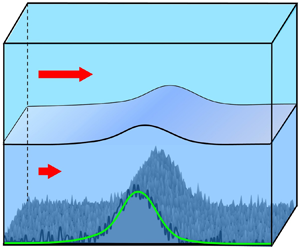
Striving to expand the applicability of the sandpaper theory, we now proceed to develop the next-generation model based on a multilayer shallow-water system. The resulting parameterization is tested using the configuration in figure 2, which depicts an externally forced stratified flow interacting with a corrugated meridional ridge – a set-up motivated by the observations in figure 1. The parametric simulations are compared with the corresponding roughness-resolving experiments. Their close agreement instils confidence in the ability of the sandpaper model to represent challenging systems, inaccessible by quasi-geostrophic models.

Figure 2. The set-up of the simulations used for testing the sandpaper theory. An externally forced current impinges on a large-scale ridge, which is represented by the Gaussian pattern (green curve) perturbed by irregular small-scale variability (black curve).
The material is organized as follows. Section 2 presents the governing equations. In § 3, we describe the stratified sandpaper theory and the resulting explicit parameterization of roughness. This parameterization is then validated by topography-resolving simulations (§ 4). The results are summarized, and conclusions are drawn, in § 5.
2. Formulation
The n-layer shallow-water model (e.g. Pedlosky Reference Pedlosky1987) includes the (x, y) momentum and thickness equations
 \begin{align}\left.
{\begin{array}{*{20}{c}} {\dfrac{{\partial
\boldsymbol{v}_i^\ast }}{{\partial {t^\ast }}} +
(\boldsymbol{v}_i^\ast \boldsymbol{\cdot
}\boldsymbol{\nabla })\boldsymbol{v}_i^\ast + {f^\ast
}\boldsymbol{k} \times \boldsymbol{v}_i^\ast = -
\dfrac{1}{{\rho_0^\ast }}\boldsymbol{\nabla }p_i^\ast +
{\upsilon^\ast }{\nabla^2}\boldsymbol{v}_i^\ast +
\boldsymbol{F}_i^\ast - {\delta_{n\,\,i}}\gamma_b^\ast
\dfrac{{\boldsymbol{v}_i^\ast }}{{h_i^\ast }} +
{\delta_{1\,\,i}}\dfrac{{{\boldsymbol{\tau }^\ast
}}}{{\rho_0^\ast h_i^\ast }},}\\ {\dfrac{{\partial h_i^\ast
}}{{\partial {t^\ast }}} + \boldsymbol{\nabla
}\boldsymbol{\cdot }(\boldsymbol{v}_i^\ast h_i^\ast ) =
E_i^\ast ,} \end{array}}
\right\}\end{align}
\begin{align}\left.
{\begin{array}{*{20}{c}} {\dfrac{{\partial
\boldsymbol{v}_i^\ast }}{{\partial {t^\ast }}} +
(\boldsymbol{v}_i^\ast \boldsymbol{\cdot
}\boldsymbol{\nabla })\boldsymbol{v}_i^\ast + {f^\ast
}\boldsymbol{k} \times \boldsymbol{v}_i^\ast = -
\dfrac{1}{{\rho_0^\ast }}\boldsymbol{\nabla }p_i^\ast +
{\upsilon^\ast }{\nabla^2}\boldsymbol{v}_i^\ast +
\boldsymbol{F}_i^\ast - {\delta_{n\,\,i}}\gamma_b^\ast
\dfrac{{\boldsymbol{v}_i^\ast }}{{h_i^\ast }} +
{\delta_{1\,\,i}}\dfrac{{{\boldsymbol{\tau }^\ast
}}}{{\rho_0^\ast h_i^\ast }},}\\ {\dfrac{{\partial h_i^\ast
}}{{\partial {t^\ast }}} + \boldsymbol{\nabla
}\boldsymbol{\cdot }(\boldsymbol{v}_i^\ast h_i^\ast ) =
E_i^\ast ,} \end{array}}
\right\}\end{align}
where  $\boldsymbol{v}_i^\ast = (u_i^\ast ,v_i^\ast )$ is the lateral velocity in layer $i = 1, \ldots ,n$, which is assumed to be vertically uniform, $p_i^\ast $ is pressure, $\rho _0^\ast $ is the reference density of the Boussinesq approximation, ${\upsilon ^\ast }$ is the eddy viscosity, ${f^\ast }$ is the Coriolis parameter, $\boldsymbol{k}$ is the vertical unit vector, ${\delta _{i\,j}}$ is the Kronecker delta, ${\boldsymbol{\tau }^\ast } = (\tau _x^\ast ,\tau _y^\ast )$ is the wind stress and $\gamma _b^\ast $–the bottom drag coefficient. The asterisks denote dimensional quantities, and the interfacial drag $\boldsymbol{F}_i^\ast = (F_{x\;i}^\ast ,F_{y\;i}^\ast )$ represents frictional effects due to the interaction of layer i with layers above (i − 1) and below (i + 1)
 \begin{equation}\left. {\begin{array}{*{20}{c}} {\boldsymbol{F}_1^\ast = \dfrac{{{\gamma^\ast }}}{{h_i^\ast }}(\boldsymbol{v}_2^\ast - \boldsymbol{v}_1^\ast ),}\\ {\boldsymbol{F}_i^\ast = \dfrac{{{\gamma^\ast }}}{{h_i^\ast }}(\boldsymbol{v}_{i + 1}^\ast + \boldsymbol{v}_{i - 1}^\ast - 2\boldsymbol{v}_i^\ast ),\quad i = 2, \ldots ,n - 1,}\\ {\boldsymbol{F}_n^\ast = \dfrac{{{\gamma^\ast }}}{{h_i^\ast }}(\boldsymbol{v}_{n - 1}^\ast - \boldsymbol{v}_n^\ast ),} \end{array}} \right\}\end{equation}
where  ${\gamma ^\ast }$ is the interfacial drag coefficient. Term $E_i^\ast $ in the thickness equation captures the modification of the water-mass composition by diapycnal mixing. One of the commonly used representations of diapycnal mixing in multilayer models is based on the McDougall and Dewar (Reference McDougall and Dewar1998) framework, which expresses $E_i^\ast $ in terms of layer depths and the effective vertical eddy diffusivity ( $k_\rho ^\ast $)
 \begin{equation}E_i^\ast = k_\rho ^\ast e_i^\ast (h_{i - 1}^\ast ,h_i^\ast ,h_{i + 1}^\ast ).\end{equation}
 It should also be noted that the bottom drag model used in this study – and in all mainstream oceanic general circulation models as well – differs from the original Ekman friction model. The systematic analysis of the Ekman boundary layer over variable topography leads to a more complex and, somewhat counterintuitively, nonlinear drag model (Zavala Sansón and van Heijst Reference Zavala Sansón and van Heijst2002). Since the Ekman theory assumes uniform eddy viscosity, which may not be realized in the ocean, most numerical and theoretical investigations opt for a simpler bottom drag parameterization (2.1). The drag coefficient  $\gamma _b^\ast $ could be either constant (linear drag model) or proportional to the flow speed (nonlinear model).
Another essential component of the multilayer shallow-water model is the hydrostatic approximation, which makes it possible to connect the dynamic pressure in the adjacent layers
 \begin{equation}p_i^\ast = p_{i + 1}^\ast + g(\rho _{i + 1}^\ast - \rho _i^\ast )H_i^\ast ,\quad H_i^\ast = \sum\limits_{j = 1}^i {h_j^\ast } ,\end{equation}
where g is the gravity. We also adopt the rigid-lid approximation for the sea surface, which implies that the water column depth  $H_n^\ast $ does not vary in time. This, in turn, demands that
 \begin{equation}\sum\limits_{i = 1}^n {\boldsymbol{\nabla }\boldsymbol{\cdot }(\boldsymbol{v}_i^\ast h_i^\ast )} = 0.\end{equation}
To reduce the number of controlling parameters, the governing equations are non-dimensionalized as follows:
 \begin{align}\boldsymbol{v}_i^\ast = f_0^\ast {L^\ast }{\boldsymbol{v}_i},\quad p_i^\ast = \rho _0^\ast {(f_0^\ast {L^\ast })^2}{p_i},\quad ({x^\ast },{y^\ast }) = {L^\ast }(x,y),\quad {t^\ast } = \frac{t}{{f_0^\ast }},\quad h_i^\ast = H_0^\ast {h_i},\end{align}
where  ${L^\ast }$, $H_0^\ast $ and $f_0^\ast $ are the representative scales for the width of small-scale topographic features, the ocean depth and the Coriolis parameter, respectively. To be specific, we consider the oceanographically relevant scales of
 \begin{equation}{L^\ast } = {10^4}\ \textrm{m},\quad H_0^\ast = 4000\ \textrm{m},\quad f_0^\ast = {10^{ - 4}}\ \textrm{s}{}^{ - 1}.\end{equation}
The non-dimensional momentum and thickness equations take the form
 \begin{equation}\left.
{\begin{array}{*{20}{c}} \dfrac{{\partial
{\boldsymbol{v}_i}}}{{\partial t}} +
({\boldsymbol{v}_i}\boldsymbol{\cdot }\boldsymbol{\nabla
}){\boldsymbol{v}_i} + f\boldsymbol{k} \times
{\boldsymbol{v}_i} = - \boldsymbol{\nabla }{p_i} +
\upsilon {\nabla^2}{\boldsymbol{v}_i}\\ \quad +\, {\boldsymbol{F}_i}
-
{\delta_{n\,\,i}}{\gamma_b}\dfrac{{{\boldsymbol{v}_i}}}{{{h_i}}}
+ {\delta_{1\,\,i}}\dfrac{\boldsymbol{\tau }}{{{h_i}}}\\
{\dfrac{{\partial {h_i}}}{{\partial t}} +
\boldsymbol{\nabla }\boldsymbol{\cdot
}({\boldsymbol{v}_i}{h_i}) = {k_\rho }{e_i}} \end{array}}
\right\}\quad i = 1, \ldots
,n,\end{equation}
\begin{equation}\left.
{\begin{array}{*{20}{c}} \dfrac{{\partial
{\boldsymbol{v}_i}}}{{\partial t}} +
({\boldsymbol{v}_i}\boldsymbol{\cdot }\boldsymbol{\nabla
}){\boldsymbol{v}_i} + f\boldsymbol{k} \times
{\boldsymbol{v}_i} = - \boldsymbol{\nabla }{p_i} +
\upsilon {\nabla^2}{\boldsymbol{v}_i}\\ \quad +\, {\boldsymbol{F}_i}
-
{\delta_{n\,\,i}}{\gamma_b}\dfrac{{{\boldsymbol{v}_i}}}{{{h_i}}}
+ {\delta_{1\,\,i}}\dfrac{\boldsymbol{\tau }}{{{h_i}}}\\
{\dfrac{{\partial {h_i}}}{{\partial t}} +
\boldsymbol{\nabla }\boldsymbol{\cdot
}({\boldsymbol{v}_i}{h_i}) = {k_\rho }{e_i}} \end{array}}
\right\}\quad i = 1, \ldots
,n,\end{equation}where
 \begin{align}{\boldsymbol{F}_i} =
\frac{{\boldsymbol{F}_i^\ast }}{{{L^\ast }f_0^{{\ast}
2}}},\quad \boldsymbol{\tau } = \frac{{{\boldsymbol{\tau
}^\ast }}}{{\rho _0^\ast {L^\ast }f_0^{{\ast} 2}H_0^\ast
}},\quad \upsilon = \frac{{{\upsilon ^\ast }}}{{{L^{{\ast}
2}}f_0^\ast }},\quad {k_\rho } = \frac{{k_\rho ^\ast
}}{{H_0^\ast {L^\ast }f_0^\ast }},\quad \textrm{(}\gamma
,{\gamma _b}\textrm{)} = \frac{{\textrm{(}{\gamma ^\ast
},\gamma _b^\ast \textrm{)}}}{{f_0^\ast H_0^\ast
}}.\end{align}
\begin{align}{\boldsymbol{F}_i} =
\frac{{\boldsymbol{F}_i^\ast }}{{{L^\ast }f_0^{{\ast}
2}}},\quad \boldsymbol{\tau } = \frac{{{\boldsymbol{\tau
}^\ast }}}{{\rho _0^\ast {L^\ast }f_0^{{\ast} 2}H_0^\ast
}},\quad \upsilon = \frac{{{\upsilon ^\ast }}}{{{L^{{\ast}
2}}f_0^\ast }},\quad {k_\rho } = \frac{{k_\rho ^\ast
}}{{H_0^\ast {L^\ast }f_0^\ast }},\quad \textrm{(}\gamma
,{\gamma _b}\textrm{)} = \frac{{\textrm{(}{\gamma ^\ast
},\gamma _b^\ast \textrm{)}}}{{f_0^\ast H_0^\ast
}}.\end{align}The recursive relation (2.4) reduces in non-dimensional units to
 \begin{equation}{p_i} = {p_{i + 1}} + {B_i}{H_i},\quad i = 1,\ldots ,n - 1, \end{equation}
where  ${B_i} = g(\rho _{i + 1}^\ast - \rho _i^\ast )H_0^\ast{/}\rho _0^\ast {(f_0^\ast {L^\ast })^2}$ is the Burger number.
Guided by the analytical treatment of rough topography in the barotropic sandpaper model (Radko Reference Radko2023b), we base our analysis on the potential vorticity (PV) equation for the bottom layer. The PV equation is obtained by taking the curl of the momentum equations (2.8) for i = n, which eliminates the pressure gradient terms, and combining it with the corresponding thickness equation
 \begin{equation}\frac{{\partial q}}{{\partial t}} + {u_n}\frac{{\partial q}}{{\partial x}} + {v_n}\frac{{\partial q}}{{\partial y}} = {F_q}. \end{equation}
 The relative and potential vorticities in the bottom layer are denoted as  $\varsigma $ and q, respectively,
 \begin{equation}\varsigma = \frac{{\partial {v_n}}}{{\partial x}} - \frac{{\partial {u_n}}}{{\partial y}},\quad q = \frac{{f + \varsigma }}{{{h_n}}},\end{equation}
and the right-hand side of (2.11) represents the cumulative effect of all dissipative processes affecting the Lagrangian conservation of PV
 \begin{equation}{F_q} = \upsilon \frac{{{\nabla ^2}\varsigma }}{{{h_n}}} - \frac{{{\gamma _b}}}{{{h_n}}}\frac{\partial }{{\partial x}}\left( {\frac{{{v_n}}}{{{h_n}}}} \right) + \frac{{{\gamma _b}}}{{{h_n}}}\frac{\partial }{{\partial y}}\left( {\frac{{{u_n}}}{{{h_n}}}} \right) + \frac{1}{{{h_n}}}\frac{{\partial {F_{y\;n}}}}{{\partial x}} - \frac{1}{{{h_n}}}\frac{{\partial {F_{x\;n}}}}{{\partial y}} - {k_\rho }\frac{{{e_n}}}{{h_n^2}}(\varsigma + f).\end{equation}
To explore the interaction between flow components of large and small lateral extent, we introduce the scale-separation parameter
 \begin{equation}\varepsilon = \frac{{{L_C}}}{{{L_{LS}}}} \ll 1,\end{equation}
where LLS is the representative lateral extent of the large-scale flow, and LC is the cutoff value that separates scales that we intend to resolve from those that we wish to parameterize. Parameter  $\varepsilon $ defines the new set of spatial scales (X,Y) that reflects the dynamics of large-scale processes. The large-scale variables are related to the original ones as follows:
 \begin{equation}(X,Y) = \varepsilon (x,y), \end{equation}
and the derivatives in the governing equations are replaced accordingly
 \begin{equation}\frac{\partial }{{\partial x}} \to \frac{\partial }{{\partial x}} + \varepsilon \frac{\partial }{{\partial X}},\quad \frac{\partial }{{\partial y}} \to \frac{\partial }{{\partial y}} + \varepsilon \frac{\partial }{{\partial Y}}.\end{equation}
 We consider topographic patterns  $\eta = 1 - {H_n}$ that vary on both large and small scales
 \begin{equation}\eta = {\eta _L}(X,Y) + {\eta _S}(x,y).\end{equation}
As in the earlier versions of the sandpaper theory (Radko Reference Radko2023a,Reference Radkob), we separate bathymetry into the small-scale and large-scale components using the Fourier transform of  $\eta $
 \begin{equation}\eta = \frac{{\sqrt {{L_x}{L_y}} }}{{2{\rm \pi} }}\iint {\tilde{\eta }(k,l)\,\textrm{exp}(\textrm{i}kx + \textrm{i}ly)\,\textrm{d}k\,\textrm{d}l} ,\end{equation}
where  $(k,l)$ are the wavenumbers in x and y, respectively, tildes hereafter denote Fourier images and $({L_x},{L_y})$ is the domain size. The normalization factor $\sqrt {{L_x}{L_y}} /2{\rm \pi} $ in (2.18) is introduced to ensure that the Parseval identity (Parseval Reference Parseval1806), used in subsequent developments, takes a convenient form
 \begin{equation}\langle ab\rangle = \iint {\tilde{a} \cdot \textrm{conj}(\tilde{b})\,\textrm{d}k\,\textrm{d}l} .\end{equation}
The angle brackets hereafter represent averaging over small-scale variables and primes denote the deviation from them:  $a^{\prime} \equiv a - \langle a\rangle $. The contributions from high and low wavenumbers to the net topographic variability are defined as follows:
 \begin{equation}\begin{aligned} \eta & = \underbrace{{\dfrac{{\sqrt {{L_x}{L_y}} }}{{2{\rm \pi} }}\int_{\kappa < 2{\rm \pi} /{L_C}} {\tilde{\eta }(k,l)\,\textrm{exp}(\textrm{i}kx + \textrm{i}ly)\,\textrm{d}k\,\textrm{d}l} }}_{{{\eta _L}}}\\ & \quad + \underbrace{{\dfrac{{\sqrt {{L_x}{L_y}} }}{{2{\rm \pi} }}\iint_{\kappa > 2{\rm \pi} /{L_C}} {\tilde{\eta }(k,l)\,\textrm{exp}(\textrm{i}kx + \textrm{i}ly)\,\textrm{d}k\,\textrm{d}l} }}_{{{\eta _S}}}, \end{aligned}\end{equation}
 where  $\kappa \equiv \sqrt {{k^2} + {l^2}} $. The ${\eta _L}$ component in (2.20) gently varies on relatively large scales, and ${\eta _S}$ represents small-scale variability. Without loss of generality, we insist that $\langle {\eta _S}\rangle = 0$ and ${\eta ^{\prime}_L} = 0\,.$
3. The multiscale analysis
In this section, we develop the large-scale evolutionary model using methods of multiscale mechanics (e.g. Mei and Vernescu Reference Mei and Vernescu2010). Our earlier explorations (Radko Reference Radko2023a,Reference Radkob) reveal substantial differences in the topographic regulation of relatively slow and fast flows. Thus, we shall separately consider the asymptotic limits of high and low Reynolds numbers (Re), defined as
 \begin{equation}Re = \frac{{{U^\ast }{L^\ast }}}{{{\upsilon ^\ast }}},\end{equation}
where  ${U^\ast }$ is the representative large-scale velocity.
3.1. Fast flows
The limit of large  $( \sim {\varepsilon ^{ - 1}})$ Reynolds numbers is captured by considering the asymptotic sector $U = O(1)$ and $\upsilon = O(\varepsilon )$. The temporal variable is rescaled as $T = \varepsilon t$ – the time scale set by advective processes operating on large spatial scales – and the time derivatives in governing equations are replaced accordingly
 \begin{equation}\frac{\partial }{{\partial t}} \to \varepsilon \frac{\partial }{{\partial T}}.\end{equation}
We open the expansion with the order-one large-scale flow. The velocity field in the deepest layer is represented by
 \begin{equation}{\boldsymbol{v}_n} = \boldsymbol{v}_n^{(0)}(X,Y,T) + \varepsilon \boldsymbol{v}_n^{(1)}(X,Y,x,y,T) + {\varepsilon ^2}\boldsymbol{v}_n^{(2)}(X,Y,x,y,T) + \cdots.\end{equation}
The corresponding pressure field takes the form
 \begin{align}{p_n} = {\varepsilon ^{ - 2}}p_n^{( - 2)}(T) + {\varepsilon ^{ - 1}}p_n^{( - 1)}(X,Y,T) + p_n^{(0)}(X,Y,T) + \varepsilon p_n^{(1)}(X,Y,x,y,T) + \cdots,\end{align}
and the analogous notation is used for the PV (q) series. The leading-order component  $p_n^{( - 2)}$ is laterally uniform and therefore does not directly affect the velocity field. It is included to represent the potential vertical drift of interfaces due to the entrainment of water masses in adjacent layers.
We anticipate that a different solution will be found in the upper layers ( $i < n$). These regions are shielded from the direct influence of bottom roughness and therefore small-scale variability appears in $\textrm{(}{\boldsymbol{v}_i},{p_i}\textrm{)}$ fields only at $O\textrm{(}{\varepsilon ^2}\textrm{)}$. The Coriolis parameter ( $f$) is a function of the large-scale latitudinal coordinate only: $f = f(Y)$. The parameters controlling the intensity of dissipative processes are rescaled as follows:
 \begin{equation}\upsilon = \varepsilon {\upsilon _0},\quad {k_\rho } = \varepsilon {k_{\rho 0}},\quad (\gamma ,{\gamma _b}) = {\varepsilon ^3}({\gamma _0},{\gamma _{b0}}).\end{equation}
Note that the horizontal and vertical friction coefficients are rescaled differently. This scaling places their direct effects on large-scale flows at the same level – at  $O\textrm{(}{\varepsilon ^3}\textrm{)}$ – in the expansion of the momentum equations, which streamlines the model development. However, we mention in passing that the sandpaper theory can be formulated even when $(\gamma ,{\gamma _b})$ are introduced at a lower order. Such an approach was taken, for instance, by Radko (Reference Radko2022a,Reference Radkob), albeit at the expense of some asymptotic untidiness in the model development. Importantly, all our earlier efforts consistently indicated that vertical friction contributes to the sandpaper effect less than lateral friction for the oceanographically relevant parameters. Hence, we proceed with scaling (3.5), which permits a rigorous analytical treatment.
The small-scale bathymetric variability is assumed to be of relatively low amplitude
 \begin{equation}{\eta _S} = \varepsilon {\eta _{S0}}.\end{equation}
In this study, we consider representative configurations in which the first baroclinic Rossby radius of deformation  $R_d^\ast \sim (1/f_0^\ast )\sqrt {g(\varDelta {\rho ^\ast }/\rho _0^\ast )H_0^\ast } $ greatly exceeds the roughness scale. Thus, we assume that ${L^\ast }\sim \varepsilon R_d^\ast $, which suggests rescaling the Burger number as follows:
 \begin{equation}{B_i} = {\varepsilon ^{ - 2}}B_i^{(0)}.\end{equation}
For the interface immediately above the bottom layer, (3.7) transforms (2.10) into
 \begin{equation}{H_{n - 1}} = \frac{{{\varepsilon ^2}}}{{B_{n - 1}^{(0)}}}({p_{n - 1}} - {p_n}),\end{equation}
which implies that Hn −1 varies rather gently in space
 \begin{align}{H_{n - 1}} = H_{n - 1}^{(0)}(T) + \varepsilon H_{n - 1}^{(1)}(X,Y,T) + {\varepsilon ^2}H_{n - 1}^{(2)}(X,Y,T) + {\varepsilon ^3}H_{n - 1}^{(3)}(X,Y,x,y,T) + \cdots ,\end{align}
with small-scale variability relegated to  $O\textrm{(}{\varepsilon ^3}\textrm{)}$. Such a limited imprint of small-scale topography on density interfaces is consistent with our earlier estimates of the vertical extent ( $h_{eff}^\ast $) of the region directly impacted by roughness (Radko Reference Radko2022b). In the continuously stratified model, $h_{eff}^\ast \sim {f^\ast }/({N^\ast }\kappa _S^\ast),$ where ${N^\ast }\sim \sqrt {\varDelta {\rho ^\ast }g/(\rho _0^\ast H_0^\ast) }$ is the buoyancy frequency and $\kappa _S^\ast $ is the representative wavenumber of small-scale topography. When this estimate is expressed in terms of the radius of deformation, we arrive at $h_{eff}^\ast \sim {L^\ast }H_0^\ast{/}(2{\rm \pi} R_d^\ast)$. Thus, as long as ${L^\ast } \ll R_d^\ast $ and $h_n^\ast \sim H_0^\ast $, we conclude that $h_{eff}^\ast \ll h_n^\ast $, which implies that bottom roughness cannot effectively perturb the interface $z = - {H_{n - 1}}$.
Such a weak small-scale variability of interfaces, in turn, has critical ramifications for the bottom layer  ${h_n} = 1 - \eta - {H_{n - 1}}$. In particular, (3.9) demands that ${h_n}$ takes the form
 \begin{align}{h_n} &= h_n^{(0)}(X,Y,T)
+ \varepsilon h_n^{(1)}(X,Y,T) - \varepsilon {\eta
_{S0}}(x,y) + {\varepsilon ^2}h_n^{(2)}(X,Y,T)\nonumber\\ &\quad +
{\varepsilon ^3}h_n^{(3)}(X,Y,x,y,T) + \cdots.
\end{align}
\begin{align}{h_n} &= h_n^{(0)}(X,Y,T)
+ \varepsilon h_n^{(1)}(X,Y,T) - \varepsilon {\eta
_{S0}}(x,y) + {\varepsilon ^2}h_n^{(2)}(X,Y,T)\nonumber\\ &\quad +
{\varepsilon ^3}h_n^{(3)}(X,Y,x,y,T) + \cdots.
\end{align}The relatively gentle spatial variation of density interfaces also implies that the properly discretized vertical buoyancy gradients and associated cross-layer entrainment velocities follow the same pattern
 \begin{align}{e_i} = e_i^{(0)}(X,Y,T) + \varepsilon e_i^{(1)}(X,Y,T) + {\varepsilon ^2}e_i^{(2)}(X,Y,T) + {\varepsilon ^3}e_i^{(3)}(X,Y,x,y,T) + \cdots .\end{align}
 We now substitute all power series in the governing equations and collect terms of the same order. The critical insights into the dynamics of flow–topography interaction are brought by the analysis of the PV equation (2.11). Its O(1) balance is trivially satisfied, whereas at  $O(\varepsilon )$ we arrive at
 \begin{equation}\frac{{\partial {q^{(0)}}}}{{\partial T}} + u_n^{(0)}\frac{{\partial {q^{(1)}}}}{{\partial x}} + v_n^{(0)}\frac{{\partial {q^{(1)}}}}{{\partial y}} + u_n^{(0)}\frac{{\partial {q^{(0)}}}}{{\partial X}} + v_n^{(0)}\frac{{\partial {q^{(0)}}}}{{\partial Y}} = 0,\end{equation}
where  ${q^{(0)}} = f/h_n^{(0)}$ and
 \begin{equation}{q^{(1)}} = \frac{1}{{h_n^{(0)}}}\left( {\frac{{\partial v^{\prime(1)}_n}}{{\partial x}} - \frac{{\partial u^{\prime(1)}_n}}{{\partial y}} + \frac{{\partial v_n^{(0)}}}{{\partial X}} - \frac{{\partial u_n^{(0)}}}{{\partial Y}}} \right) + \frac{{f({\eta _{S0}} - h_n^{(1)})}}{{{{(v)}^2}}}.\end{equation}
Averaging (3.12) in  $(x,y)$ leads to
 \begin{equation}\frac{{\partial {q^{(0)}}}}{{\partial T}} + u_n^{(0)}\frac{{\partial {q^{(0)}}}}{{\partial X}} + v_n^{(0)}\frac{{\partial {q^{(0)}}}}{{\partial Y}} = 0,\end{equation}
which is readily recognized as the leading-order Lagrangian conservation of PV. However, after subtracting (3.12) and (3.14), we also arrive at the diagnostic condition
 \begin{equation}u_n^{(0)}\frac{{\partial {q^{(1)}}}}{{\partial x}} + v_n^{(0)}\frac{{\partial {q^{(1)}}}}{{\partial y}} = 0.\end{equation}
This requirement is satisfied by insisting that  ${q^{(1)}}$ does not vary on small spatial scales
 \begin{equation}{q^{(1)}} = {q^{(1)}}(X,Y,T).\end{equation}
Statement (3.16) reflects the tendency for small-scale homogenization of PV, a well-known phenomenon affecting the dynamics of numerous geophysical systems (e.g. Rhines and Young Reference Rhines and Young1982; Dewar Reference Dewar1986; Marshall et al. Reference Marshall, Williams and Lee1999). Potential vorticity homogenization has also been unambiguously identified as the key mechanism controlling flow–topography interaction in our previous studies (Radko Reference Radko2022a,Reference Radkob, Reference Radko2023a,Reference Radkob; Gulliver and Radko Reference Gulliver and Radko2023).
The lack of small-scale variability in the first-order PV field (3.13) demands that  ${q^{\prime(1)}} = 0$, which in turn requires
 \begin{equation}\frac{{\partial v^{\prime(1)}_n}}{{\partial x}} - \frac{{\partial u^{\prime(1)}_n}}{{\partial y}} + \frac{{f{\eta _{S0}}}}{{h_n^{(0)}}} = 0, \end{equation}
and reduces (3.13) to
 \begin{equation}{q^{(1)}} = \frac{1}{{h_n^{(0)}}}\left( {\frac{{\partial v_n^{(0)}}}{{\partial X}} - \frac{{\partial u_n^{(0)}}}{{\partial Y}}} \right) - \frac{{fh_n^{(1)}}}{{{{(h_n^{(0)})}^2}}}.\end{equation}
The treatment of the second-order components of the PV equation is similar. We establish the  $O({\varepsilon ^2})$ balance, subtract its small-scale average and simplify the result using (3.17)
 \begin{align}u_n^{(0)}\frac{{\partial {{q^{\prime}}^{(2)}}}}{{\partial x}} + v_n^{(0)}\frac{{\partial {{q^{\prime}}^{(2)}}}}{{\partial y}} = - u^{\prime(1)}_n\frac{{\partial {q^{(0)}}}}{{\partial X}} - v^{\prime(1)}_n\frac{{\partial {q^{(0)}}}}{{\partial Y}} - \frac{{{\upsilon _0}}}{{{{(h_n^{(0)})}^2}}}{\nabla ^2}(f{\eta _{S0}}) - {k_{\rho 0}}{e_0}\frac{{f{\eta _{S0}}}}{{{{(h_n^{(0)})}^3}}}.\end{align}
Equation (3.19) represents a critical step in the development of the sandpaper theory. It explicitly links the second-order PV perturbations to the small-scale bathymetric pattern. These PV perturbations are expressed in terms of velocities as follows:
 \begin{equation}{q^{\prime(2)}} = \frac{1}{{h_n^{(0)}}}\left( {\frac{{\partial v^{\prime(2)}_n}}{{\partial x}} - \frac{{\partial u^{\prime(2)}_n}}{{\partial y}} + \frac{{\partial v^{\prime(1)}_n}}{{\partial X}} - \frac{{\partial u^{\prime(1)}_n}}{{\partial Y}}} \right) + \frac{{{\eta _{S0}}{q^{(1)}}}}{{{{(h_n^{(0)})}^2}}}.\end{equation}
 We now turn our attention to the thickness equation. Its leading-order balance is realized at  $O(\varepsilon )$
 \begin{gather}
\dfrac{{\partial h_n^{(0)}}}{{\partial T}} +
\dfrac{\partial }{{\partial x}}(u_n^{(0)}h_n^{(1)} -
u_n^{(0)}{\eta _{S0}} + u_n^{(1)}h_n^{(0)}) +
\dfrac{\partial }{{\partial y}}(v_n^{(0)}h_n^{(1)} -
v_n^{(0)}{\eta _{S0}} + v_n^{(1)}h_n^{(0)})\nonumber\\
\qquad\quad +\, \dfrac{\partial }{{\partial X}}(u_n^{(0)}h_n^{(0)}) +
\dfrac{\partial }{{\partial Y}}(v_n^{(0)}h_n^{(0)}) =
{k_{\rho 0}}e_n^{(0)}.
\end{gather}
\begin{gather}
\dfrac{{\partial h_n^{(0)}}}{{\partial T}} +
\dfrac{\partial }{{\partial x}}(u_n^{(0)}h_n^{(1)} -
u_n^{(0)}{\eta _{S0}} + u_n^{(1)}h_n^{(0)}) +
\dfrac{\partial }{{\partial y}}(v_n^{(0)}h_n^{(1)} -
v_n^{(0)}{\eta _{S0}} + v_n^{(1)}h_n^{(0)})\nonumber\\
\qquad\quad +\, \dfrac{\partial }{{\partial X}}(u_n^{(0)}h_n^{(0)}) +
\dfrac{\partial }{{\partial Y}}(v_n^{(0)}h_n^{(0)}) =
{k_{\rho 0}}e_n^{(0)}.
\end{gather}
When this balance is averaged in  $(x,y)$ and the result is subtracted from (3.21), we arrive at
 \begin{equation}\frac{\partial }{{\partial x}}( - u_n^{(0)}{\eta _{S0}} + u^{\prime(1)}_nh_n^{(0)}) + \frac{\partial }{{\partial y}}( - v_n^{(0)}{\eta _{S0}} + v^{\prime(1)}_nh_n^{(0)}) = 0.\end{equation}
Combining (3.22) and (3.17) makes it possible to compute the first-order perturbation velocity
 \begin{equation}\left. {\begin{array}{*{20}{c}} {{\nabla^2}u^{\prime(1)}_n = \dfrac{1}{{h_n^{(0)}}}\left( {u_n^{(0)}\dfrac{{{\partial^2}{\eta_{S0}}}}{{\partial {x^2}}} + v_n^{(0)}\dfrac{{{\partial^2}{\eta_{S0}}}}{{\partial x\partial y}} + f\dfrac{{\partial {\eta_{S0}}}}{{\partial y}}} \right),}\\ {{\nabla^2}v^{\prime(1)}_n = \dfrac{1}{{h_n^{(0)}}}\left( {u_n^{(0)}\dfrac{{{\partial^2}{\eta_{S0}}}}{{\partial x\partial y}} + v_n^{(0)}\dfrac{{{\partial^2}{\eta_{S0}}}}{{\partial {y^2}}} - f\dfrac{{\partial {\eta_{S0}}}}{{\partial x}}} \right).} \end{array}} \right\}\end{equation}
The first two terms on the right-hand sides of both expressions represent the fundamentally ageostrophic processes that are not considered in the quasi-geostrophic version of the sandpaper theory (Radko Reference Radko2023a). One of the key objectives of the present study is the assessment of the role played by these ageostrophic effects in the interaction between large-scale flows and rough topography.
The second-order balance of the thickness equation (not shown) is treated similarly, but the third-order balance of the thickness equation reveals a new and interesting dynamics. Its small-scale average amounts to
 \begin{gather}
\dfrac{{\partial h_n^{(2)}}}{{\partial T}} +
\dfrac{\partial }{{\partial X}}(u_n^{(0)}h_n^{(2)} +
\langle u_n^{(1)}\rangle h_n^{(1)} + \langle
u_n^{(2)}\rangle h_n^{(0)} - \langle u^{\prime(1)}_n{\eta
_{S0}}\rangle )\nonumber\\
+\, \dfrac{\partial }{{\partial
Y}}(v_n^{(0)}h_n^{(2)} + \langle v_n^{(1)}\rangle h_n^{(1)}
+ \langle v_n^{(2)}\rangle h_n^{(0)} - \langle
v^{\prime(1)}_n{\eta _{S0}}\rangle ) = {k_{\rho
0}}e_n^{(2)}.
\end{gather}
\begin{gather}
\dfrac{{\partial h_n^{(2)}}}{{\partial T}} +
\dfrac{\partial }{{\partial X}}(u_n^{(0)}h_n^{(2)} +
\langle u_n^{(1)}\rangle h_n^{(1)} + \langle
u_n^{(2)}\rangle h_n^{(0)} - \langle u^{\prime(1)}_n{\eta
_{S0}}\rangle )\nonumber\\
+\, \dfrac{\partial }{{\partial
Y}}(v_n^{(0)}h_n^{(2)} + \langle v_n^{(1)}\rangle h_n^{(1)}
+ \langle v_n^{(2)}\rangle h_n^{(0)} - \langle
v^{\prime(1)}_n{\eta _{S0}}\rangle ) = {k_{\rho
0}}e_n^{(2)}.
\end{gather}
The key feature of (3.24) is the appearance of eddy-transfer terms  $\langle u^{\prime(1)}_n{\eta _{S0}}\rangle$ and $\langle v^{\prime(1)}_n{\eta _{S0}}\rangle$ that directly influence the evolution of the large-scale thickness field. The treatment of these terms is based on the transformed Eulerian mean (TEM) framework (e.g. Andrews and McIntyre Reference Andrews and Mcintyre1976), which reformulates the conservation equations in terms of a residual circulation that includes the effect of both mean flow and eddies. Following the principal tenet of the TEM theory, we introduce the residual-mean velocities
 \begin{equation}\boldsymbol{v}_{res}^{(2)} = \langle \boldsymbol{v}_n^{(2)}\rangle - \frac{{\langle {\boldsymbol{v}^{\prime}}_n^{(1)}{\eta _{S0}}\rangle }}{{h_n^{(0)}}}.\end{equation}
 In this study, we consider statistically isotropic seafloor patterns with power spectra that are uniquely determined by the absolute wavenumber:  ${|{{{\tilde{\eta }}_{S0}}} |^2} = S(\kappa )$. For such patterns, the eddy-transfer components in (3.25) can be conveniently linked to the leading-order velocities using (3.23) as follows:
 \begin{equation}\langle {\boldsymbol{v}^{\prime}}_n^{(1)}{\eta _{S0}}\rangle = \frac{{{\alpha _{10}}\boldsymbol{v}_n^{(0)}}}{{h_n^{(0)}}},\quad {\alpha _{10}} = \frac{1}{2}\langle \eta _{S0}^2\rangle = {\rm \pi} \int {{{|{{{\tilde{\eta }}_{S0}}} |}^2}\kappa \,\textrm{d}\kappa } .\end{equation}
The residual-mean formulation (3.25) makes it possible to reduce (3.24) to
 \begin{align}\frac{{\partial
h_n^{(2)}}}{{\partial T}} & + \frac{\partial }{{\partial
X}}(u_n^{(0)}h_n^{(2)} + \langle u_n^{(1)}\rangle h_n^{(1)}
+ u_{res}^{(2)}h_n^{(0)}) + \frac{\partial }{{\partial
Y}}(v_n^{(0)}h_n^{(2)}\nonumber\\ &\quad + \langle v_n^{(1)}\rangle h_n^{(1)}
+ v_{res}^{(2)}h_n^{(0)}) = {k_{\rho
0}}e_n^{(2)},\end{align}
\begin{align}\frac{{\partial
h_n^{(2)}}}{{\partial T}} & + \frac{\partial }{{\partial
X}}(u_n^{(0)}h_n^{(2)} + \langle u_n^{(1)}\rangle h_n^{(1)}
+ u_{res}^{(2)}h_n^{(0)}) + \frac{\partial }{{\partial
Y}}(v_n^{(0)}h_n^{(2)}\nonumber\\ &\quad + \langle v_n^{(1)}\rangle h_n^{(1)}
+ v_{res}^{(2)}h_n^{(0)}) = {k_{\rho
0}}e_n^{(2)},\end{align}which, as will be seen shortly, leads to several technical and conceptual simplifications.
The fourth-order balance of the averaged thickness equation is similarly expressed in terms of residual velocities as follows:
 \begin{gather}
\dfrac{{\partial \langle h_n^{(3)}\rangle }}{{\partial T}}
+ \dfrac{\partial }{{\partial X}}(u_n^{(0)}\langle
h_n^{(3)}\rangle + \langle u_n^{(1)}\rangle h_n^{(2)} +
u_{res}^{(2)}h_n^{(1)} + u_{res}^{(3)}h_n^{(0)})\nonumber\\
+\, \dfrac{\partial }{{\partial Y}}(v_n^{(0)}\langle
h_n^{(3)}\rangle + \langle v_n^{(1)}\rangle h_n^{(2)} +
v_{res}^{(2)}h_n^{(1)} + v_{res}^{(3)}h_n^{(0)}) = {k_{\rho
0}}\langle e_n^{(3)}\rangle ,
\end{gather}
\begin{gather}
\dfrac{{\partial \langle h_n^{(3)}\rangle }}{{\partial T}}
+ \dfrac{\partial }{{\partial X}}(u_n^{(0)}\langle
h_n^{(3)}\rangle + \langle u_n^{(1)}\rangle h_n^{(2)} +
u_{res}^{(2)}h_n^{(1)} + u_{res}^{(3)}h_n^{(0)})\nonumber\\
+\, \dfrac{\partial }{{\partial Y}}(v_n^{(0)}\langle
h_n^{(3)}\rangle + \langle v_n^{(1)}\rangle h_n^{(2)} +
v_{res}^{(2)}h_n^{(1)} + v_{res}^{(3)}h_n^{(0)}) = {k_{\rho
0}}\langle e_n^{(3)}\rangle ,
\end{gather}where
 \begin{equation}\boldsymbol{v}_{res}^{(3)} = \langle {\boldsymbol{v}}_n^{(3)}\rangle + \frac{{\langle {\boldsymbol{v}^{\prime}}_n^{(1)}{\eta _{S0}}\rangle }}{{{{(h_n^{(0)})}^2}}}h_n^{(1)} - \frac{{\langle {\boldsymbol{v}^{\prime}}_n^{(2)}{\eta _{S0}}\rangle }}{{h_n^{(0)}}}.\end{equation}
 Finally, we proceed with the analysis of the momentum equations. At  $O(1)$, we arrive at the geostrophic balance for large-scale components
 \begin{equation}\left.
{\begin{array}{*{20}{c}} {fv_n^{(0)} = \dfrac{{\partial
p_n^{( - 1)}}}{{\partial X}},}\\ {fu_n^{(0)} = -
\dfrac{{\partial p_n^{( - 1)}}}{{\partial Y}}.}
\end{array}}
\right\}\end{equation}
\begin{equation}\left.
{\begin{array}{*{20}{c}} {fv_n^{(0)} = \dfrac{{\partial
p_n^{( - 1)}}}{{\partial X}},}\\ {fu_n^{(0)} = -
\dfrac{{\partial p_n^{( - 1)}}}{{\partial Y}}.}
\end{array}}
\right\}\end{equation} At  $O(\varepsilon )$, the $(x,y)$-averaged equations represent the dominant advective large-scale processes
 \begin{equation}\left.
{\begin{array}{*{20}{c}} {\dfrac{{\partial
u_n^{(0)}}}{{\partial T}} + u_n^{(0)}\dfrac{{\partial
u_n^{(0)}}}{{\partial X}} + v_n^{(0)}\dfrac{{\partial
u_n^{(0)}}}{{\partial Y}} - f\langle v_n^{(1)}\rangle = -
\dfrac{{\partial p_n^{(0)}}}{{\partial X}},}\\
{\dfrac{{\partial v_n^{(0)}}}{{\partial T}} +
u_n^{(0)}\dfrac{{\partial v_n^{(0)}}}{{\partial X}} +
v_n^{(0)}\dfrac{{\partial v_n^{(0)}}}{{\partial Y}} +
f\langle u_n^{(1)}\rangle = - \dfrac{{\partial
p_n^{(0)}}}{{\partial Y}}.} \end{array}}
\right\}\end{equation}
\begin{equation}\left.
{\begin{array}{*{20}{c}} {\dfrac{{\partial
u_n^{(0)}}}{{\partial T}} + u_n^{(0)}\dfrac{{\partial
u_n^{(0)}}}{{\partial X}} + v_n^{(0)}\dfrac{{\partial
u_n^{(0)}}}{{\partial Y}} - f\langle v_n^{(1)}\rangle = -
\dfrac{{\partial p_n^{(0)}}}{{\partial X}},}\\
{\dfrac{{\partial v_n^{(0)}}}{{\partial T}} +
u_n^{(0)}\dfrac{{\partial v_n^{(0)}}}{{\partial X}} +
v_n^{(0)}\dfrac{{\partial v_n^{(0)}}}{{\partial Y}} +
f\langle u_n^{(1)}\rangle = - \dfrac{{\partial
p_n^{(0)}}}{{\partial Y}}.} \end{array}}
\right\}\end{equation}
We note that large-scale equations (3.30) and (3.31) also appear in the widely used quasi-geostrophic model (e.g. Charney Reference Charney1948, Reference Charney1971; Pedlosky Reference Pedlosky1987). The key distinction is that quasi-geostrophy also assumes small variations in layer depths, which is not required in the present formulation. The  $O({\varepsilon ^2})$ balance of the averaged momentum equations takes the form
 \begin{equation}\left.
{\begin{array}{*{20}{c}} {\dfrac{{\partial \langle
u_n^{(1)}\rangle }}{{\partial {t_1}}} + A_u^{(2)} +
\left\langle {v^{\prime(1)}_n\dfrac{{\partial
u^{\prime(1)}_n}}{{\partial y}}} \right\rangle - f\langle
v_n^{(2)}\rangle = - \dfrac{{\partial \langle
p_n^{(1)}\rangle }}{{\partial X}},}\\ {\dfrac{{\partial
\langle v_n^{(1)}\rangle }}{{\partial {t_1}}} + A_v^{(2)} +
\left\langle {u^{\prime(1)}_n\dfrac{{\partial
v^{\prime(1)}_n}}{{\partial x}}} \right\rangle + f\langle
u_n^{(2)}\rangle = - \dfrac{{\partial \langle
p_n^{(1)}\rangle }}{{\partial Y}},} \end{array}}
\right\}\end{equation}
\begin{equation}\left.
{\begin{array}{*{20}{c}} {\dfrac{{\partial \langle
u_n^{(1)}\rangle }}{{\partial {t_1}}} + A_u^{(2)} +
\left\langle {v^{\prime(1)}_n\dfrac{{\partial
u^{\prime(1)}_n}}{{\partial y}}} \right\rangle - f\langle
v_n^{(2)}\rangle = - \dfrac{{\partial \langle
p_n^{(1)}\rangle }}{{\partial X}},}\\ {\dfrac{{\partial
\langle v_n^{(1)}\rangle }}{{\partial {t_1}}} + A_v^{(2)} +
\left\langle {u^{\prime(1)}_n\dfrac{{\partial
v^{\prime(1)}_n}}{{\partial x}}} \right\rangle + f\langle
u_n^{(2)}\rangle = - \dfrac{{\partial \langle
p_n^{(1)}\rangle }}{{\partial Y}},} \end{array}}
\right\}\end{equation}
where  $A_u^{(2)}$ and $A_v^{(2)}$ are the second-order mean-field advection terms
 \begin{equation}\left.
{\begin{array}{*{20}{c}} {A_u^{(2)} =
u_n^{(0)}\dfrac{{\partial \langle u_n^{(1)}\rangle
}}{{\partial X}} + \langle u_n^{(1)}\rangle
\dfrac{{\partial u_n^{(0)}}}{{\partial X}} +
v_n^{(0)}\dfrac{{\partial \langle u_n^{(1)}\rangle
}}{{\partial Y}} + \langle v_n^{(1)}\rangle
\dfrac{{\partial u_n^{(0)}}}{{\partial Y}},}\\ {A_v^{(2)} =
u_n^{(0)}\dfrac{{\partial \langle v_n^{(0)}\rangle
}}{{\partial X}} + \langle u_n^{(1)}\rangle
\dfrac{{\partial v_n^{(0)}}}{{\partial X}} +
v_n^{(0)}\dfrac{{\partial \langle v_n^{(1)}\rangle
}}{{\partial Y}} + \langle v_n^{(1)}\rangle
\dfrac{{\partial v_n^{(0)}}}{{\partial Y}}.} \end{array}}
\right\}\end{equation}
\begin{equation}\left.
{\begin{array}{*{20}{c}} {A_u^{(2)} =
u_n^{(0)}\dfrac{{\partial \langle u_n^{(1)}\rangle
}}{{\partial X}} + \langle u_n^{(1)}\rangle
\dfrac{{\partial u_n^{(0)}}}{{\partial X}} +
v_n^{(0)}\dfrac{{\partial \langle u_n^{(1)}\rangle
}}{{\partial Y}} + \langle v_n^{(1)}\rangle
\dfrac{{\partial u_n^{(0)}}}{{\partial Y}},}\\ {A_v^{(2)} =
u_n^{(0)}\dfrac{{\partial \langle v_n^{(0)}\rangle
}}{{\partial X}} + \langle u_n^{(1)}\rangle
\dfrac{{\partial v_n^{(0)}}}{{\partial X}} +
v_n^{(0)}\dfrac{{\partial \langle v_n^{(1)}\rangle
}}{{\partial Y}} + \langle v_n^{(1)}\rangle
\dfrac{{\partial v_n^{(0)}}}{{\partial Y}}.} \end{array}}
\right\}\end{equation} The dynamics reflected by (3.32) requires some interpretation. The presence of finite Reynolds stress terms  $\langle v_n^{\prime(1)}(\partial u_n^{\prime(1)}/\partial y)\rangle$ and $\langle u_n^{\prime(1)}(\partial v_n^{\prime(1)}/\partial x)\rangle$ seems to indicate that topography can influence large-scale evolution at $O({\varepsilon ^2})$ through the eddy-induced transfer of momentum. Some reflection, however, casts doubt on this proposition. The Reynolds stress terms can be expressed, using (3.23), in terms of basic velocities
 \begin{equation}\left\langle
{v_n^{\prime(1)}\frac{{\partial u_n^{\prime(1)}}}{{\partial y}}}
\right\rangle = \frac{{{\alpha
_{10}}v_n^{(0)}f}}{{{{(h_n^{(0)})}^2}}},\quad \left\langle
{u_n^{\prime(1)}\frac{{\partial v_n^{\prime(1)}}}{{\partial x}}}
\right\rangle = - \frac{{{\alpha
_{10}}u_n^{(0)}f}}{{{{(h_n^{(0)})}^2}}}.\end{equation}
\begin{equation}\left\langle
{v_n^{\prime(1)}\frac{{\partial u_n^{\prime(1)}}}{{\partial y}}}
\right\rangle = \frac{{{\alpha
_{10}}v_n^{(0)}f}}{{{{(h_n^{(0)})}^2}}},\quad \left\langle
{u_n^{\prime(1)}\frac{{\partial v_n^{\prime(1)}}}{{\partial x}}}
\right\rangle = - \frac{{{\alpha
_{10}}u_n^{(0)}f}}{{{{(h_n^{(0)})}^2}}}.\end{equation}When we substitute (3.34) and (3.25) in (3.32), the result is
 \begin{equation}\left.
{\begin{array}{*{20}{c}} {\dfrac{{\partial \langle
u_n^{(1)}\rangle }}{{\partial T}} + A_u^{(2)} - f\langle
v_{res}^{(2)}\rangle = - \dfrac{{\partial \langle
p_n^{(1)}\rangle }}{{\partial X}},}\\ {\dfrac{{\partial
\langle v_n^{(1)}\rangle }}{{\partial T}} + A_v^{(2)} +
f\langle u_{res}^{(2)}\rangle = - \dfrac{{\partial \langle
p_n^{(1)}\rangle }}{{\partial Y}}.} \end{array}}
\right\}\end{equation}
\begin{equation}\left.
{\begin{array}{*{20}{c}} {\dfrac{{\partial \langle
u_n^{(1)}\rangle }}{{\partial T}} + A_u^{(2)} - f\langle
v_{res}^{(2)}\rangle = - \dfrac{{\partial \langle
p_n^{(1)}\rangle }}{{\partial X}},}\\ {\dfrac{{\partial
\langle v_n^{(1)}\rangle }}{{\partial T}} + A_v^{(2)} +
f\langle u_{res}^{(2)}\rangle = - \dfrac{{\partial \langle
p_n^{(1)}\rangle }}{{\partial Y}}.} \end{array}}
\right\}\end{equation}
System (3.35) indicates that the Reynolds stress terms do not explicitly appear in the residual-mean (rather than Eulerian) momentum equations at  $O({\varepsilon ^2})$. This finding suggests the leading-order cancellation of the net effects of the eddy-induced transport of momentum and thickness. Thus, to quantify the tangible impact of small scales on large-scale patterns, we must analyse the $O({\varepsilon ^3})$ momentum balance.
The (x, y)-averaged third-order momentum equations are
 \begin{equation}\left.
{\begin{array}{*{20}{c}} \dfrac{{\partial \langle
u_n^{(2)}\rangle }}{{\partial T}} + A_u^{(3)} + R_u^{(3)} -
{f}\langle v_n^{(3)}\rangle = - \dfrac{{\partial \langle
p_n^{(2)}\rangle }}{{\partial X}} + {\nu_0}\left(
{\dfrac{{{\partial^2}u_n^{(0)}}}{{\partial {X^2}}} +
\dfrac{{{\partial^2}u_n^{(0)}}}{{\partial {Y^2}}}} \right)\\
\quad +\, {\gamma_0}\dfrac{{u_{n - 1}^{(0)} -
u_n^{(0)}}}{{h_n^{(0)}}} -
{\gamma_{b0}}\dfrac{{u_n^{(0)}}}{{h_n^{(0)}}},\\
\dfrac{{\partial \langle v_n^{(2)}\rangle }}{{\partial T}}
+ A_v^{(3)} + R_v^{(3)} + {f}\langle u_n^{(3)}\rangle
= - \dfrac{{\partial \langle p_n^{(2)}\rangle }}{{\partial
Y}} + {\nu_0}\left(
{\dfrac{{{\partial^2}v_n^{(0)}}}{{\partial {X^2}}} +
\dfrac{{{\partial^2}v_n^{(0)}}}{{\partial {Y^2}}}} \right) \\
\quad +\, {\gamma_0}\dfrac{{v_{n - 1}^{(0)} -
v_n^{(0)}}}{{h_n^{(0)}}} -
{\gamma_{b0}}\dfrac{{v_n^{(0)}}}{{h_n^{(0)}}},
\end{array}}
\right\}\end{equation}
\begin{equation}\left.
{\begin{array}{*{20}{c}} \dfrac{{\partial \langle
u_n^{(2)}\rangle }}{{\partial T}} + A_u^{(3)} + R_u^{(3)} -
{f}\langle v_n^{(3)}\rangle = - \dfrac{{\partial \langle
p_n^{(2)}\rangle }}{{\partial X}} + {\nu_0}\left(
{\dfrac{{{\partial^2}u_n^{(0)}}}{{\partial {X^2}}} +
\dfrac{{{\partial^2}u_n^{(0)}}}{{\partial {Y^2}}}} \right)\\
\quad +\, {\gamma_0}\dfrac{{u_{n - 1}^{(0)} -
u_n^{(0)}}}{{h_n^{(0)}}} -
{\gamma_{b0}}\dfrac{{u_n^{(0)}}}{{h_n^{(0)}}},\\
\dfrac{{\partial \langle v_n^{(2)}\rangle }}{{\partial T}}
+ A_v^{(3)} + R_v^{(3)} + {f}\langle u_n^{(3)}\rangle
= - \dfrac{{\partial \langle p_n^{(2)}\rangle }}{{\partial
Y}} + {\nu_0}\left(
{\dfrac{{{\partial^2}v_n^{(0)}}}{{\partial {X^2}}} +
\dfrac{{{\partial^2}v_n^{(0)}}}{{\partial {Y^2}}}} \right) \\
\quad +\, {\gamma_0}\dfrac{{v_{n - 1}^{(0)} -
v_n^{(0)}}}{{h_n^{(0)}}} -
{\gamma_{b0}}\dfrac{{v_n^{(0)}}}{{h_n^{(0)}}},
\end{array}}
\right\}\end{equation}
where  $A_u^{(3)}$ and $A_v^{(3)}$ represent the mean-flow advection
 \begin{equation}\left.
\begin{array}{*{20}{c}} A_u^{(3)} = \langle
u_n^{(2)}\rangle \dfrac{{\partial u_n^{(0)}}}{{\partial X}}
+ \langle u_n^{(1)}\rangle \dfrac{{\partial \langle
u_n^{(1)}\rangle }}{{\partial X}} +
u_n^{(0)}\dfrac{{\partial \langle u_n^{(2)}\rangle
}}{{\partial X}} + \langle v_n^{(2)}\rangle
\dfrac{{\partial u_n^{(0)}}}{{\partial Y}}\\ \quad +\, \langle
v_n^{(1)}\rangle \dfrac{{\partial \langle u_n^{(1)}\rangle
}}{{\partial Y}} + v_n^{(0)}\dfrac{{\partial \langle
u_n^{(2)}\rangle }}{{\partial Y}},\\ A_v^{(3)} = \langle
u_n^{(2)}\rangle \dfrac{{\partial v_n^{(0)}}}{{\partial X}}
+ \langle u_n^{(1)}\rangle \dfrac{{\partial \langle
v_n^{(1)}\rangle }}{{\partial X}} +
u_n^{(0)}\dfrac{{\partial \langle v_n^{(2)}\rangle
}}{{\partial X}} + \langle v_n^{(2)}\rangle
\dfrac{{\partial v_n^{(0)}}}{{\partial Y}}\\ \quad +\, \langle
v_n^{(1)}\rangle \dfrac{{\partial \langle v_n^{(1)}\rangle
}}{{\partial Y}} + v_n^{(0)}\dfrac{{\partial \langle
v_n^{(2)}\rangle }}{{\partial Y}}, \end{array}
\right\}\end{equation}
\begin{equation}\left.
\begin{array}{*{20}{c}} A_u^{(3)} = \langle
u_n^{(2)}\rangle \dfrac{{\partial u_n^{(0)}}}{{\partial X}}
+ \langle u_n^{(1)}\rangle \dfrac{{\partial \langle
u_n^{(1)}\rangle }}{{\partial X}} +
u_n^{(0)}\dfrac{{\partial \langle u_n^{(2)}\rangle
}}{{\partial X}} + \langle v_n^{(2)}\rangle
\dfrac{{\partial u_n^{(0)}}}{{\partial Y}}\\ \quad +\, \langle
v_n^{(1)}\rangle \dfrac{{\partial \langle u_n^{(1)}\rangle
}}{{\partial Y}} + v_n^{(0)}\dfrac{{\partial \langle
u_n^{(2)}\rangle }}{{\partial Y}},\\ A_v^{(3)} = \langle
u_n^{(2)}\rangle \dfrac{{\partial v_n^{(0)}}}{{\partial X}}
+ \langle u_n^{(1)}\rangle \dfrac{{\partial \langle
v_n^{(1)}\rangle }}{{\partial X}} +
u_n^{(0)}\dfrac{{\partial \langle v_n^{(2)}\rangle
}}{{\partial X}} + \langle v_n^{(2)}\rangle
\dfrac{{\partial v_n^{(0)}}}{{\partial Y}}\\ \quad +\, \langle
v_n^{(1)}\rangle \dfrac{{\partial \langle v_n^{(1)}\rangle
}}{{\partial Y}} + v_n^{(0)}\dfrac{{\partial \langle
v_n^{(2)}\rangle }}{{\partial Y}}, \end{array}
\right\}\end{equation}
while  $R_u^{(3)}$ and $R_v^{(3)}$ are the Reynolds stresses associated with small-scale topographic forcing
 \begin{equation}\left.
{\begin{array}{*{20}{c}} R_u^{(3)} = \left\langle
{u^{\prime(2)}_n\dfrac{{\partial
u^{\prime(1)}_n}}{{\partial x}}} \right\rangle +
\left\langle {u^{\prime(1)}_n\dfrac{{\partial
u^{\prime(2)}_n}}{{\partial x}}} \right\rangle +
\left\langle {u^{\prime(1)}_n\dfrac{{\partial
u^{\prime(1)}_n}}{{\partial X}}} \right\rangle +
\left\langle {v^{\prime(2)}_n\dfrac{{\partial
u^{\prime(1)}_n}}{{\partial y}}} \right\rangle\\ \quad +\,
\left\langle {v^{\prime(1)}_n\dfrac{{\partial
u^{\prime(2)}_n}}{{\partial y}}} \right\rangle +
\left\langle {v^{\prime(1)}_n\dfrac{{\partial
u^{\prime(1)}_n}}{{\partial Y}}} \right\rangle ,\\
R_v^{(3)} = \left\langle {u^{\prime(2)}_n\dfrac{{\partial
v^{\prime(1)}_n}}{{\partial x}}} \right\rangle +
\left\langle {u^{\prime(1)}_n\dfrac{{\partial
v^{\prime(2)}_n}}{{\partial x}}} \right\rangle +
\left\langle {u^{\prime(1)}_n\dfrac{{\partial
v^{\prime(1)}_n}}{{\partial X}}} \right\rangle +
\left\langle {v^{\prime(2)}_n\dfrac{{\partial
v^{\prime(1)}_n}}{{\partial y}}} \right\rangle\\ \quad +
\left\langle {v^{\prime(1)}_n\dfrac{{\partial
v^{\prime(2)}_n}}{{\partial y}}} \right\rangle +
\left\langle {v^{\prime(1)}_n\dfrac{{\partial
v^{\prime(1)}_n}}{{\partial Y}}} \right\rangle .
\end{array}}
\right\}\end{equation}
\begin{equation}\left.
{\begin{array}{*{20}{c}} R_u^{(3)} = \left\langle
{u^{\prime(2)}_n\dfrac{{\partial
u^{\prime(1)}_n}}{{\partial x}}} \right\rangle +
\left\langle {u^{\prime(1)}_n\dfrac{{\partial
u^{\prime(2)}_n}}{{\partial x}}} \right\rangle +
\left\langle {u^{\prime(1)}_n\dfrac{{\partial
u^{\prime(1)}_n}}{{\partial X}}} \right\rangle +
\left\langle {v^{\prime(2)}_n\dfrac{{\partial
u^{\prime(1)}_n}}{{\partial y}}} \right\rangle\\ \quad +\,
\left\langle {v^{\prime(1)}_n\dfrac{{\partial
u^{\prime(2)}_n}}{{\partial y}}} \right\rangle +
\left\langle {v^{\prime(1)}_n\dfrac{{\partial
u^{\prime(1)}_n}}{{\partial Y}}} \right\rangle ,\\
R_v^{(3)} = \left\langle {u^{\prime(2)}_n\dfrac{{\partial
v^{\prime(1)}_n}}{{\partial x}}} \right\rangle +
\left\langle {u^{\prime(1)}_n\dfrac{{\partial
v^{\prime(2)}_n}}{{\partial x}}} \right\rangle +
\left\langle {u^{\prime(1)}_n\dfrac{{\partial
v^{\prime(1)}_n}}{{\partial X}}} \right\rangle +
\left\langle {v^{\prime(2)}_n\dfrac{{\partial
v^{\prime(1)}_n}}{{\partial y}}} \right\rangle\\ \quad +
\left\langle {v^{\prime(1)}_n\dfrac{{\partial
v^{\prime(2)}_n}}{{\partial y}}} \right\rangle +
\left\langle {v^{\prime(1)}_n\dfrac{{\partial
v^{\prime(1)}_n}}{{\partial Y}}} \right\rangle .
\end{array}}
\right\}\end{equation} Our goal is to explicitly connect the Reynolds stresses (3.38) to large-scale properties. We shall start with  $R_u^{(3)}$. The first two terms in $R_u^{(3)}$ are combined and then eliminated by virtue of identity $(\partial /\partial x)(u^{\prime(1)}_nu^{\prime(2)}_n) = u^{\prime(2)}_n(\partial /\partial x)u^{\prime(1)}_n + u^{\prime(1)}_n(\partial /\partial x)u^{\prime(2)}_n$, and the third term is written as $(\partial /\partial X)\langle {\textstyle{1 \over 2}}{(u^{\prime(1)}_n)^2}\rangle$. The remaining terms are expressed in terms of PV components using (3.17) and (3.20)
 \begin{align}R_u^{(3)} =
\frac{\partial }{{\partial X}}\left\langle
{\frac{{{{(u^{\prime(1)}_n)}^2} +
{{(v^{\prime(1)}_n)}^2}}}{2}} \right\rangle + \langle
v^{\prime(1)}_n{\eta _{S0}}\rangle {q^{(1)}} - \langle
v^{\prime(1)}_n{q^{\prime(2)}}\rangle h_n^{(0)} + \langle
v^{\prime(2)}_n{\eta _{S0}}\rangle
{q^{(0)}}.\end{align}
\begin{align}R_u^{(3)} =
\frac{\partial }{{\partial X}}\left\langle
{\frac{{{{(u^{\prime(1)}_n)}^2} +
{{(v^{\prime(1)}_n)}^2}}}{2}} \right\rangle + \langle
v^{\prime(1)}_n{\eta _{S0}}\rangle {q^{(1)}} - \langle
v^{\prime(1)}_n{q^{\prime(2)}}\rangle h_n^{(0)} + \langle
v^{\prime(2)}_n{\eta _{S0}}\rangle
{q^{(0)}}.\end{align}
The principal complication in evaluating (3.39) is presented by term  ${R_q} = - \langle v^{\prime(1)}_n{q^{\prime(2)}}\rangle h_n^{(0)}$. The technical difficulty here is that the PV equation (3.19) provides only the along-flow variation in ${q^{\prime(2)}}$. To surmount this problem and compute ${R_q}$ using (3.19), we follow the methodology implemented in the previous versions of the sandpaper theory (e.g. Radko Reference Radko2023b). First, we apply the Parseval identity
 \begin{equation}\langle v^{\prime(1)}_n{q^{\prime(2)}}\rangle = \iint {\tilde{v^{\prime}}_n^{(1)} \cdot \textrm{conj}({{\tilde{q^{\prime}}}^{(2)}})\,\textrm{d}k\,\textrm{d}l} ,\end{equation}
and then adopt the flow-following coordinate system
 \begin{equation}\left.
{\begin{array}{*{20}{c@{}}} {\hat{k} = k\,\textrm{cos}\,\theta
+ l\,\textrm{sin}\,\theta ,}\\ {\hat{l} = -
k\,\textrm{sin}\,\theta + l\,\textrm{cos}\,\theta .}
\end{array}}
\right\}\end{equation}
\begin{equation}\left.
{\begin{array}{*{20}{c@{}}} {\hat{k} = k\,\textrm{cos}\,\theta
+ l\,\textrm{sin}\,\theta ,}\\ {\hat{l} = -
k\,\textrm{sin}\,\theta + l\,\textrm{cos}\,\theta .}
\end{array}}
\right\}\end{equation}
The flow-orientation variable  $\theta $ in (3.41) is defined by
 \begin{equation}\textrm{cos}(\theta ) = \frac{{u_n^{(0)}}}{{{V_0}}},\quad \textrm{sin}(\theta ) = \frac{{v_n^{(0)}}}{{{V_0}}},\end{equation}
where  ${V_0} = \sqrt {{{(u_n^{(0)})}^2} + {{(v_n^{(0)})}^2}}$. The transition to the flow-following coordinate system greatly simplifies the treatment of ${q^{\prime(2)}}$. We apply the Fourier transform to the PV equation (3.19). In the flow-following coordinate system, the Fourier transform of its left-hand side $(u_n^{(0)}(\partial {q^{\prime(2)}}/\partial x) + v_n^{(0)}(\partial {q^{\prime(2)}}/\partial y))$ is remarkably concise: ${V_0}{\kern 1pt} \hat{k}\,{\tilde{q}^{\prime(2)}}$. This simplification leads to an explicit expression for ${\tilde{q}^{\prime}_2}$, which is then used to evaluate (3.40) and thereby determine ${R_q}$
 \begin{equation}{R_q} = \frac{{{\alpha _{20}}{f^2}}}{{{{(h_n^{(0)})}^3}}}\frac{{\partial h_n^{(0)}}}{{\partial X}} + \frac{{2\upsilon {\alpha _{10}}u_n^{(0)}{f^2}}}{{V_0^2{{(h_n^{(0)})}^2}}} - {k_\rho }{\alpha _{20}}\frac{{u_n^{(0)}{f^2}e_n^{(0)}}}{{V_0^2{{(h_n^{(0)})}^3}}},\end{equation}
where  ${\alpha _{20}} = 2{\rm \pi} \int {{{|{{{\tilde{\eta }}_{S0}}} |}^2}{\kappa ^{ - 1}}\,\textrm{d}\kappa }$.
The final step in deriving the large-scale evolutionary x-momentum equation is the transition from Eulerian large-scale velocities to their residual counterparts using (3.25) and (3.29)
 \begin{gather}
\dfrac{\partial }{{\partial T}}\left( {u_{res}^{(2)} +
\dfrac{{{\alpha_1}u_n^{(0)}}}{{{{(h_n^{(0)})}^2}}}} \right)
+ A_{u\;res}^{(3)} + D_{u\;fast}^{(3)} - {f_0}\langle
v_{res}^{(3)}\rangle\nonumber \\
= - \dfrac{{\partial
\langle p_n^{(2)}\rangle }}{{\partial X}} + {\nu _0}\left(
{\dfrac{{{\partial^2}u_n^{(0)}}}{{\partial {X^2}}} +
\dfrac{{{\partial^2}u_n^{(0)}}}{{\partial {Y^2}}}} \right)
+ {\gamma _0}\dfrac{{u_{n - 1}^{(0)} -
u_n^{(0)}}}{{h_n^{(0)}}} - {\gamma
_{b0}}\dfrac{{u_n^{(0)}}}{{h_n^{(0)}}},
\end{gather}
\begin{gather}
\dfrac{\partial }{{\partial T}}\left( {u_{res}^{(2)} +
\dfrac{{{\alpha_1}u_n^{(0)}}}{{{{(h_n^{(0)})}^2}}}} \right)
+ A_{u\;res}^{(3)} + D_{u\;fast}^{(3)} - {f_0}\langle
v_{res}^{(3)}\rangle\nonumber \\
= - \dfrac{{\partial
\langle p_n^{(2)}\rangle }}{{\partial X}} + {\nu _0}\left(
{\dfrac{{{\partial^2}u_n^{(0)}}}{{\partial {X^2}}} +
\dfrac{{{\partial^2}u_n^{(0)}}}{{\partial {Y^2}}}} \right)
+ {\gamma _0}\dfrac{{u_{n - 1}^{(0)} -
u_n^{(0)}}}{{h_n^{(0)}}} - {\gamma
_{b0}}\dfrac{{u_n^{(0)}}}{{h_n^{(0)}}},
\end{gather}where
 \begin{align}A_{u_{res}}^{(3)} =
u_{res}^{(2)}\frac{{\partial u_n^{(0)}}}{{\partial X}} +
\langle u_n^{(1)}\rangle \frac{{\partial \langle
u_n^{(1)}\rangle }}{{\partial X}} +
u_n^{(0)}\frac{{\partial u_{res}^{(2)}}}{{\partial X}} +
v_{res}^{(2)}\frac{{\partial u_n^{(0)}}}{{\partial Y}} +
\langle v_n^{(1)}\rangle \frac{{\partial \langle
u_n^{(1)}\rangle }}{{\partial Y}} +
v_n^{(0)}\frac{{\partial u_{res}^{(2)}}}{{\partial
Y}},\end{align}
\begin{align}A_{u_{res}}^{(3)} =
u_{res}^{(2)}\frac{{\partial u_n^{(0)}}}{{\partial X}} +
\langle u_n^{(1)}\rangle \frac{{\partial \langle
u_n^{(1)}\rangle }}{{\partial X}} +
u_n^{(0)}\frac{{\partial u_{res}^{(2)}}}{{\partial X}} +
v_{res}^{(2)}\frac{{\partial u_n^{(0)}}}{{\partial Y}} +
\langle v_n^{(1)}\rangle \frac{{\partial \langle
u_n^{(1)}\rangle }}{{\partial Y}} +
v_n^{(0)}\frac{{\partial u_{res}^{(2)}}}{{\partial
Y}},\end{align}and
 \begin{align}
D_{u\;fast}^{(3)} & = \dfrac{{{\alpha
_{10}}}}{{{{(h_n^{(0)})}^3}}}\left(
{3u_n^{(0)}h_n^{(0)}\dfrac{{\partial u_n^{(0)}}}{{\partial
X}} - 3{{(u_n^{(0)})}^2}\dfrac{{\partial
h_n^{(0)}}}{{\partial X}} +
2v_n^{(0)}h_n^{(0)}\dfrac{{\partial v_n^{(0)}}}{{\partial
X}} - {{(v_n^{(0)})}^2}\dfrac{{\partial
h_n^{(0)}}}{{\partial X}}} \right)\nonumber\\
& \quad +\, \dfrac{{{\alpha _{10}}}}{{{{(h_n^{(0)})}^3}}}\left(
{v_n^{(0)}h_n^{(0)}\dfrac{{\partial u_n^{(0)}}}{{\partial
Y}} - 2u_n^{(0)}v_n^{(0)}\dfrac{{\partial
h_n^{(0)}}}{{\partial Y}}} \right)\nonumber\\
&\quad +\, \dfrac{{2\upsilon
{\alpha _{10}}u_n^{(0)}{f^2}}}{{V_0^2{{(h_n^{(0)})}^2}}} -
{k_\rho }{\alpha _{20}}\dfrac{{u_n^{(0)}{f^2}e_n^{(0)}}}{{V_0^2{{(h_n^{(0)})}^3}}}.
\end{align}
\begin{align}
D_{u\;fast}^{(3)} & = \dfrac{{{\alpha
_{10}}}}{{{{(h_n^{(0)})}^3}}}\left(
{3u_n^{(0)}h_n^{(0)}\dfrac{{\partial u_n^{(0)}}}{{\partial
X}} - 3{{(u_n^{(0)})}^2}\dfrac{{\partial
h_n^{(0)}}}{{\partial X}} +
2v_n^{(0)}h_n^{(0)}\dfrac{{\partial v_n^{(0)}}}{{\partial
X}} - {{(v_n^{(0)})}^2}\dfrac{{\partial
h_n^{(0)}}}{{\partial X}}} \right)\nonumber\\
& \quad +\, \dfrac{{{\alpha _{10}}}}{{{{(h_n^{(0)})}^3}}}\left(
{v_n^{(0)}h_n^{(0)}\dfrac{{\partial u_n^{(0)}}}{{\partial
Y}} - 2u_n^{(0)}v_n^{(0)}\dfrac{{\partial
h_n^{(0)}}}{{\partial Y}}} \right)\nonumber\\
&\quad +\, \dfrac{{2\upsilon
{\alpha _{10}}u_n^{(0)}{f^2}}}{{V_0^2{{(h_n^{(0)})}^2}}} -
{k_\rho }{\alpha _{20}}\dfrac{{u_n^{(0)}{f^2}e_n^{(0)}}}{{V_0^2{{(h_n^{(0)})}^3}}}.
\end{align}
Term  $D_{u\;fast}^{(3)}$ represents the cumulative effect of seafloor roughness on large-scale flows.
The y-momentum equation is treated in a similar fashion, and the entire set of evolutionary large-scale equations is now reconstructed by combining all  $(x,y)$-averaged balances. The result is simplified by introducing the large-scale field variables as follows:
 \begin{equation}\left.
{\begin{array}{*{20}{c@{}}} {{{\bar{\boldsymbol{v}}}_n} =
\boldsymbol{v}_n^{(0)} + \varepsilon \langle
\boldsymbol{v}_n^{(1)}\rangle + {\varepsilon^2}\langle
\boldsymbol{v}_{res}^{(2)}\rangle + {\varepsilon^3}\langle
\boldsymbol{v}_{res}^{(3)}\rangle ,}\\ {{{\bar{h}}_n} =
h_n^{(0)} + \varepsilon h_n^{(1)} +
{\varepsilon^2}h_n^{(2)} + {\varepsilon^3}\langle
h_n^{(3)}\rangle .} \end{array}}
\right\}\end{equation}
\begin{equation}\left.
{\begin{array}{*{20}{c@{}}} {{{\bar{\boldsymbol{v}}}_n} =
\boldsymbol{v}_n^{(0)} + \varepsilon \langle
\boldsymbol{v}_n^{(1)}\rangle + {\varepsilon^2}\langle
\boldsymbol{v}_{res}^{(2)}\rangle + {\varepsilon^3}\langle
\boldsymbol{v}_{res}^{(3)}\rangle ,}\\ {{{\bar{h}}_n} =
h_n^{(0)} + \varepsilon h_n^{(1)} +
{\varepsilon^2}h_n^{(2)} + {\varepsilon^3}\langle
h_n^{(3)}\rangle .} \end{array}}
\right\}\end{equation}
The analogous notation is used for pressure ( ${\bar{p}_n}$), diapycnal transfer ( ${\bar{e}_n}$) and all field variables in the upper layers. At this point, we can rewrite the evolutionary large-scale equations for the bottom layer using the original independent variables $(x,y,t)$ in lieu of $(X,Y,T)$ without the risk of confusing the scales
 \begin{equation}\left.
{\begin{array}{*{20}{c}} \dfrac{\partial }{{\partial
t}}\left( {{{\bar{\boldsymbol{v}}}_n} +
{\alpha_1}\dfrac{{{{\bar{\boldsymbol{v}}}_n}}}{{\bar{h}_n^2}}}
\right) + ({{\bar{\boldsymbol{v}}}_n}\boldsymbol{\cdot
}\boldsymbol{\nabla }){{\bar{\boldsymbol{v}}}_n} +
{\boldsymbol{D}_{fast}} + f\boldsymbol{k} \times
{{\bar{\boldsymbol{v}}}_n} = - \boldsymbol{\nabla
}{{\bar{p}}_n} + \upsilon
{\nabla^2}{{\bar{\boldsymbol{v}}}_n}\\ \quad +\, \gamma
\dfrac{{{{\bar{\boldsymbol{v}}}_{n - 1}} -
{{\bar{\boldsymbol{v}}}_n}}}{{{{\bar{h}}_n}}} -
{\gamma_b}\dfrac{{{{\bar{\boldsymbol{v}}}_n}}}{{{{\bar{h}}_n}}},\\
{\dfrac{{\partial {{\bar{h}}_n}}}{{\partial t}} +
\boldsymbol{\nabla }\boldsymbol{\cdot
}({{\bar{\boldsymbol{v}}}_n}{{\bar{h}}_n}) = {k_\rho
}{{\bar{e}}_n}.} \end{array}}
\right\}\end{equation}
\begin{equation}\left.
{\begin{array}{*{20}{c}} \dfrac{\partial }{{\partial
t}}\left( {{{\bar{\boldsymbol{v}}}_n} +
{\alpha_1}\dfrac{{{{\bar{\boldsymbol{v}}}_n}}}{{\bar{h}_n^2}}}
\right) + ({{\bar{\boldsymbol{v}}}_n}\boldsymbol{\cdot
}\boldsymbol{\nabla }){{\bar{\boldsymbol{v}}}_n} +
{\boldsymbol{D}_{fast}} + f\boldsymbol{k} \times
{{\bar{\boldsymbol{v}}}_n} = - \boldsymbol{\nabla
}{{\bar{p}}_n} + \upsilon
{\nabla^2}{{\bar{\boldsymbol{v}}}_n}\\ \quad +\, \gamma
\dfrac{{{{\bar{\boldsymbol{v}}}_{n - 1}} -
{{\bar{\boldsymbol{v}}}_n}}}{{{{\bar{h}}_n}}} -
{\gamma_b}\dfrac{{{{\bar{\boldsymbol{v}}}_n}}}{{{{\bar{h}}_n}}},\\
{\dfrac{{\partial {{\bar{h}}_n}}}{{\partial t}} +
\boldsymbol{\nabla }\boldsymbol{\cdot
}({{\bar{\boldsymbol{v}}}_n}{{\bar{h}}_n}) = {k_\rho
}{{\bar{e}}_n}.} \end{array}}
\right\}\end{equation}
The terms representing the topographic forcing  ${\boldsymbol{D}_{fast}} = ({D_{u\;fast}},{D_{v\;fast}})$ contain the contributions from both advective and dissipative small-scale processes
 \begin{equation}{\boldsymbol{D}_{fast}} = {\varepsilon ^3}\boldsymbol{D}_{fast}^{(3)} = {\boldsymbol{D}^{(ad)}} + {\boldsymbol{D}^{(diss)}},\end{equation}
where
 \begin{align}\left.
{\begin{array}{*{20}{c@{}}} {D_u^{(ad)} =
\dfrac{{{\alpha_1}}}{{\bar{h}_n^3}}\left(
{3{{\bar{u}}_n}{{\bar{h}}_n}\dfrac{{\partial
{{\bar{u}}_n}}}{{\partial x}} -
3\bar{u}_n^2\dfrac{{\partial {{\bar{h}}_n}}}{{\partial x}}
+ 2{{\bar{v}}_n}{{\bar{h}}_n}\dfrac{{\partial
{{\bar{v}}_n}}}{{\partial x}} - \bar{v}_n^2\dfrac{{\partial
{{\bar{h}}_n}}}{{\partial x}} +
{{\bar{v}}_n}{{\bar{h}}_n}\dfrac{{\partial
{{\bar{u}}_n}}}{{\partial y}} -
2{{\bar{u}}_n}{{\bar{v}}_n}\dfrac{{\partial
{{\bar{h}}_n}}}{{\partial y}}} \right),}\\ {D_v^{(ad)} =
\dfrac{{{\alpha_1}}}{{\bar{h}_n^3}}\left(
{3{{\bar{v}}_n}{{\bar{h}}_n}\dfrac{{\partial
{{\bar{v}}_n}}}{{\partial y}} -
3\bar{v}_n^2\dfrac{{\partial {{\bar{h}}_n}}}{{\partial y}}
+ 2{{\bar{u}}_n}{{\bar{h}}_n}\dfrac{{\partial
{{\bar{u}}_n}}}{{\partial y}} - \bar{u}_n^2\dfrac{{\partial
{{\bar{h}}_n}}}{{\partial y}} +
{{\bar{u}}_n}{{\bar{h}}_n}\dfrac{{\partial
{{\bar{v}}_n}}}{{\partial x}} -
2{{\bar{u}}_n}{{\bar{v}}_n}\dfrac{{\partial
{{\bar{h}}_n}}}{{\partial x}}} \right),}\\
{{\boldsymbol{D}^{(diss)}} = \dfrac{{2\upsilon
{\alpha_1}{{\bar{\boldsymbol{v}}}_n}{f^2}}}{{(\bar{u}_n^2 +
\bar{v}_n^2)\bar{h}_n^2}} - \dfrac{{{k_\rho
}{\alpha_2}{{\bar{\boldsymbol{v}}}_n}{f^2}\bar{e}}}{{(\bar{u}_n^2
+ \bar{v}_n^2)\bar{h}_n^3}},} \end{array}}
\right\}\end{align}
\begin{align}\left.
{\begin{array}{*{20}{c@{}}} {D_u^{(ad)} =
\dfrac{{{\alpha_1}}}{{\bar{h}_n^3}}\left(
{3{{\bar{u}}_n}{{\bar{h}}_n}\dfrac{{\partial
{{\bar{u}}_n}}}{{\partial x}} -
3\bar{u}_n^2\dfrac{{\partial {{\bar{h}}_n}}}{{\partial x}}
+ 2{{\bar{v}}_n}{{\bar{h}}_n}\dfrac{{\partial
{{\bar{v}}_n}}}{{\partial x}} - \bar{v}_n^2\dfrac{{\partial
{{\bar{h}}_n}}}{{\partial x}} +
{{\bar{v}}_n}{{\bar{h}}_n}\dfrac{{\partial
{{\bar{u}}_n}}}{{\partial y}} -
2{{\bar{u}}_n}{{\bar{v}}_n}\dfrac{{\partial
{{\bar{h}}_n}}}{{\partial y}}} \right),}\\ {D_v^{(ad)} =
\dfrac{{{\alpha_1}}}{{\bar{h}_n^3}}\left(
{3{{\bar{v}}_n}{{\bar{h}}_n}\dfrac{{\partial
{{\bar{v}}_n}}}{{\partial y}} -
3\bar{v}_n^2\dfrac{{\partial {{\bar{h}}_n}}}{{\partial y}}
+ 2{{\bar{u}}_n}{{\bar{h}}_n}\dfrac{{\partial
{{\bar{u}}_n}}}{{\partial y}} - \bar{u}_n^2\dfrac{{\partial
{{\bar{h}}_n}}}{{\partial y}} +
{{\bar{u}}_n}{{\bar{h}}_n}\dfrac{{\partial
{{\bar{v}}_n}}}{{\partial x}} -
2{{\bar{u}}_n}{{\bar{v}}_n}\dfrac{{\partial
{{\bar{h}}_n}}}{{\partial x}}} \right),}\\
{{\boldsymbol{D}^{(diss)}} = \dfrac{{2\upsilon
{\alpha_1}{{\bar{\boldsymbol{v}}}_n}{f^2}}}{{(\bar{u}_n^2 +
\bar{v}_n^2)\bar{h}_n^2}} - \dfrac{{{k_\rho
}{\alpha_2}{{\bar{\boldsymbol{v}}}_n}{f^2}\bar{e}}}{{(\bar{u}_n^2
+ \bar{v}_n^2)\bar{h}_n^3}},} \end{array}}
\right\}\end{align}and
 \begin{equation}{\alpha _1} = {\varepsilon ^2}{\alpha _{10}} = \tfrac{1}{2}\langle \eta _S^2\rangle = {\rm \pi} \int {{{|{{{\tilde{\eta }}_S}} |}^2}\kappa \,\textrm{d}\kappa } ,\quad {\alpha _2} = {\varepsilon ^2}{\alpha _{20}} = 2{\rm \pi} \int {{{|{{{\tilde{\eta }}_S}} |}^2}{\kappa ^{ - 1}}\,\textrm{d}\kappa } .\end{equation}
While the structure of dissipative components  ${\boldsymbol{D}^{(diss)}} = (D_u^{(diss)},D_v^{(diss)})$ fully conforms to the quasi-geostrophic sandpaper model (Radko Reference Radko2023a), the advective components ${\boldsymbol{D}^{(ad)}} = (D_u^{(ad)},D_v^{(ad)})$ are fundamentally ageostrophic. Thus, a question arises regarding their relative contribution to the net topographic forcing. For the development of parameterizations, the emergence of the new advective forcing terms could be both a blessing and a curse. Component ${\boldsymbol{D}^{(ad)}}$ is well defined, whereas ${\boldsymbol{D}^{(diss)}}$ depends on the values of eddy viscosity and diffusivity $(\upsilon ,{k_\rho })$ that are poorly constrained by observations and models. Therefore, the dominance of advective forcing could open a pathway for more rigorous parameterizations of rough topography. On the other hand, a substantial magnitude of ${\boldsymbol{D}^{(ad)}}$ could bring into question the generality of conclusions based on earlier quasi-geostrophic versions of the sandpaper model.
The large-scale equations for the upper layers do not explicitly reflect the topographic forcing
 \begin{equation}\left.
{\begin{array}{*{20}{c@{}}} {\dfrac{{\partial
{{\bar{\boldsymbol{v}}}_i}}}{{\partial t}} +
({{\bar{\boldsymbol{v}}}_i}\boldsymbol{\cdot
}\boldsymbol{\nabla }){{\bar{\boldsymbol{v}}}_i} +
f\boldsymbol{k} \times {{\bar{\boldsymbol{v}}}_i} = -
\boldsymbol{\nabla }{{\bar{p}}_i} + \upsilon
{\nabla^2}{{\bar{\boldsymbol{v}}}_i} +
{{\bar{\boldsymbol{F}}}_i} +
{\delta_{1\,\,i}}\dfrac{\boldsymbol{\tau }}{{{h_i}}},}\\
{\dfrac{{\partial {{\bar{h}}_i}}}{{\partial t}} +
\boldsymbol{\nabla }\boldsymbol{\cdot
}({{\bar{\boldsymbol{v}}}_n}{{\bar{h}}_n}) = {k_\rho
}{{\bar{e}}_n},} \end{array}} \right\}\quad i = 1, \ldots
,n -
1\end{equation}
\begin{equation}\left.
{\begin{array}{*{20}{c@{}}} {\dfrac{{\partial
{{\bar{\boldsymbol{v}}}_i}}}{{\partial t}} +
({{\bar{\boldsymbol{v}}}_i}\boldsymbol{\cdot
}\boldsymbol{\nabla }){{\bar{\boldsymbol{v}}}_i} +
f\boldsymbol{k} \times {{\bar{\boldsymbol{v}}}_i} = -
\boldsymbol{\nabla }{{\bar{p}}_i} + \upsilon
{\nabla^2}{{\bar{\boldsymbol{v}}}_i} +
{{\bar{\boldsymbol{F}}}_i} +
{\delta_{1\,\,i}}\dfrac{\boldsymbol{\tau }}{{{h_i}}},}\\
{\dfrac{{\partial {{\bar{h}}_i}}}{{\partial t}} +
\boldsymbol{\nabla }\boldsymbol{\cdot
}({{\bar{\boldsymbol{v}}}_n}{{\bar{h}}_n}) = {k_\rho
}{{\bar{e}}_n},} \end{array}} \right\}\quad i = 1, \ldots
,n -
1\end{equation}although it will be shown (§ 4) that the roughness-induced modification of circulation in the bottom layer can profoundly affect the entire water column.
3.2. Regularization
The combination of (3.48) and (3.52) offers an explicit description of large-scale flows forced by rough topography. However, its implementation in theoretical and coarse-resolution numerical models is complicated by the singularity of the forcing term (3.50) in the weak flow regime:  $\bar{V} = \sqrt {\bar{u}_n^2 + \bar{v}_n^2} \to 0$. To regularize this limit, we consider asymptotic theory designed specifically for weak flows and then develop a hybrid model that encompasses the fast-flow and slow-flow limits. Two different slow-flow models, A and B, are presented. Model A is relevant for strongly dissipative systems with $Re \ll 1$. Details of this formulation are relegated to Appendix A and the key result is the explicit expression (A19) for the flow forcing by small-scale topography. Model B (Appendix B), on the other hand, does not permit a fully analytical treatment. However, it is more general and can be used for arbitrary values of Re. The resulting representations of roughness-induced drag ${\boldsymbol{D}_{slow}}$ replace ${\boldsymbol{D}_{fast}}$ in (3.48) for relatively slow flows. The forcing terms take the form
 \begin{equation}{\boldsymbol{D}_{slow}} = {G_{slow}}{\bar{\boldsymbol{v}}_n},\end{equation}
where coefficient  ${G_{slow}}$ is given in (A21) and (B17) for slow-flow models A and B, respectively. It is interesting to note that, while the fast-flow forcing (3.50) is linked to the action of the Reynolds stresses, its slow-flow counterpart (3.53) can be interpreted (Appendix A) as the ‘form drag’ caused by the pressure differences on the upstream and downstream sides of small-scale topographic features.
To represent the transition from a slow-flow to a fast-flow dynamics, we consider the hybrid model that is expected to be uniformly valid for a wide range of velocities. Importantly, we shall focus on the dissipative component of the fast-flow model  ${\boldsymbol{D}^{(diss)}}$. The advective component of the fast-flow parameterization ${\boldsymbol{D}^{(ad)}}$ is well behaved and systematically decreases with the decreasing speed of the large-scale current. Therefore, ${\boldsymbol{D}^{(ad)}}$ will be retained in its original form in the hybrid model. The analogous reasoning can be applied to term $(\partial /\partial t)({\alpha _1}({\bar{\boldsymbol{v}}_n}/\bar{h}_n^2))$ that is present in the fast-flow model (3.48) but does not appear explicitly in its slow-flow counterpart. For scales considered in the slow-flow model, this term represents a higher-order correction, and its inclusion does not compromise its asymptotic accuracy. For simplicity, $(\partial /\partial t)({\alpha _1}({\bar{\boldsymbol{v}}_n}/\bar{h}_n^2))$ is retained in the hybrid model.
Modelling the transition from  ${\boldsymbol{D}^{(diss)}}$ for fast flows to ${\boldsymbol{D}_{slow}}$ for slow ones is more challenging. While ${\boldsymbol{D}_{slow}}$ tends to increase with increasing flow speed $(\bar{V})$, ${\boldsymbol{D}^{(diss)}}$ somewhat counterintuitively decreases. Fortunately, the problem of bridging these solutions is essentially identical to the one that has already been addressed in the quasi-geostrophic sandpaper model (Radko Reference Radko2023a). To keep our discussion self-contained, we now review this approach. First, we recognize that vectors ${\boldsymbol{D}^{(diss)}}$ and ${\boldsymbol{D}_{slow}}$ are aligned with the basic current
 \begin{equation}{\boldsymbol{D}_{slow}} = {G_{slow}}\bar{V}\,\boldsymbol{s}\textrm{,}\quad {\boldsymbol{D}^{(diss)}} = {G_{fast}}{\bar{V}^{ - 1}}\,\boldsymbol{s},\end{equation}
where
 \begin{equation}{G_{fast}} = \frac{{2\upsilon {\alpha _1}{f^2}}}{{\bar{h}_n^2}} - \frac{{{k_\rho }{\alpha _2}{f^2}{{\bar{e}}_n}}}{{\bar{h}_n^3}},\end{equation}
and  $\boldsymbol{s} \equiv {\bar{\boldsymbol{v}}_n}\,{\bar{V}^{ - 1}}$ is the unit vector representing the flow direction. We connect the two regimes using the analytical function $\varPhi (\bar{V})$ that reduces to ${G_{slow}}\bar{V}\,$ and ${G_{fast}}{\bar{V}^{ - 1}}$ in the slow-flow and fast-flow limits, respectively,
 \begin{equation}\varPhi = \sqrt {{G_{slow}}{G_{fast}}} \,\textrm{exp}( - \sqrt {1 + {{\ln }^2}(\bar{V}V_C^{ - 1})} ),\end{equation}
where  ${V_C} = \sqrt {{G_{fast}}/{G_{slow}}} $ is the critical velocity marking the transition between the fast-flow and slow-flow regimes. It is defined as the crossing point of the fast-flow and slow-flow models: ${\boldsymbol{D}_{slow}}({V_C}) = {\boldsymbol{D}^{(diss)}}({V_C})$. The critical velocity also corresponds to the maximal roughness-induced drag. The hybrid model of topographic forcing is then obtained using (3.56) and adding the advection-controlled fast-flow terms
 \begin{equation}{\boldsymbol{D}_{hybrid}} = \sqrt {{G_{slow}}{G_{fast}}} \,\textrm{exp}( - \sqrt {1 + {{\ln }^2}(\bar{V}V_C^{ - 1})} )\frac{{{{\bar{\boldsymbol{v}}}_n}}}{{\bar{V}}} + {\boldsymbol{D}^{(ad)}}.\end{equation}
The corresponding evolutionary large-scale equations for the bottom layer take the form
 \begin{equation}\left.
{\begin{array}{*{20}{c}} \dfrac{\partial }{{\partial
t}}\left( {{{\bar{\boldsymbol{v}}}_n} +
{\alpha_1}\dfrac{{{{\bar{\boldsymbol{v}}}_n}}}{{\bar{h}_n^2}}}
\right) + ({{\bar{\boldsymbol{v}}}_n}\boldsymbol{\cdot
}\boldsymbol{\nabla }){{\bar{\boldsymbol{v}}}_n} +
{\boldsymbol{D}_{hybrid}} + f\,\boldsymbol{k} \times
{{\bar{\boldsymbol{v}}}_n} = - \boldsymbol{\nabla
}{{\bar{p}}_n} + \upsilon
{\nabla^2}{{\bar{\boldsymbol{v}}}_n}\\ \quad +\, \gamma
\dfrac{{{{\bar{\boldsymbol{v}}}_{n - 1}} -
{{\bar{\boldsymbol{v}}}_n}}}{{{{\bar{h}}_n}}} -
{\gamma_b}\dfrac{{{{\bar{\boldsymbol{v}}}_n}}}{{{{\bar{h}}_n}}},\\
{\dfrac{{\partial {{\bar{h}}_n}}}{{\partial t}} +
\boldsymbol{\nabla }\boldsymbol{\cdot
}({{\bar{\boldsymbol{v}}}_n}{{\bar{h}}_n}) = {k_\rho
}{{\bar{e}}_n}.} \end{array}}
\right\}\end{equation}
\begin{equation}\left.
{\begin{array}{*{20}{c}} \dfrac{\partial }{{\partial
t}}\left( {{{\bar{\boldsymbol{v}}}_n} +
{\alpha_1}\dfrac{{{{\bar{\boldsymbol{v}}}_n}}}{{\bar{h}_n^2}}}
\right) + ({{\bar{\boldsymbol{v}}}_n}\boldsymbol{\cdot
}\boldsymbol{\nabla }){{\bar{\boldsymbol{v}}}_n} +
{\boldsymbol{D}_{hybrid}} + f\,\boldsymbol{k} \times
{{\bar{\boldsymbol{v}}}_n} = - \boldsymbol{\nabla
}{{\bar{p}}_n} + \upsilon
{\nabla^2}{{\bar{\boldsymbol{v}}}_n}\\ \quad +\, \gamma
\dfrac{{{{\bar{\boldsymbol{v}}}_{n - 1}} -
{{\bar{\boldsymbol{v}}}_n}}}{{{{\bar{h}}_n}}} -
{\gamma_b}\dfrac{{{{\bar{\boldsymbol{v}}}_n}}}{{{{\bar{h}}_n}}},\\
{\dfrac{{\partial {{\bar{h}}_n}}}{{\partial t}} +
\boldsymbol{\nabla }\boldsymbol{\cdot
}({{\bar{\boldsymbol{v}}}_n}{{\bar{h}}_n}) = {k_\rho
}{{\bar{e}}_n}.} \end{array}}
\right\}\end{equation}Unlike the corresponding fast-flow model (3.48), this formulation is well posed and can be readily implemented in parametric simulations.
4. Validation
To assess the performance of the hybrid parametric model, we turn to simulations. The roughness-resolving experiments are compared with solutions based on the parameterized system (3.58). For the latter, both regularization models A and B are considered. The numerical configuration is illustrated in figure 2. The two-layer current in a zonal channel impinges on a meridional ridge. The substantial height of the ridge  $({H_L} = 1/3)$ from the outset precludes the use of quasi-geostrophic models. The upper-layer flow is maintained at the mean speed of ${U_1} = 0.1$, which is attributed to the action of the wind stress. The interfacial friction causes the lower layer, which is initially at rest, to gradually spin up. The mean thickness of the upper layer is ${H_{1\;mean}} = 0.25$ and the beta-plane model $f = {f_0} + \beta y$ is assumed for the Coriolis parameter. Other parameters are assigned values of
 \begin{equation}\gamma = {\gamma _b} = {10^{ - 3}},\quad \upsilon = 5 \times {10^{ - 3}},\quad {f_0} = 1,\quad \beta = {10^{ - 3}},\quad {k_\rho } = 0.\end{equation}
These translate in dimensional units to
 \begin{equation}\left.
{\begin{array}{*{20}{c@{}}} {U_1^\ast =
0.1\ \textrm{m}\ {\textrm{s}^{ - 1}},\quad
H_{1\ mean}^\ast = {{10}^3}\ \textrm{m},\quad H_L^\ast =
1.33 \times {{10}^3}\ \textrm{m},}\\ {\gamma^\ast } =
\gamma_b^\ast = 4 \times {{10}^{ -
4}}\ \textrm{m}\ {\textrm{s}^{ - 1}},\quad {\upsilon^\ast }
= 50\ {\textrm{m}^2}\ {\textrm{s}^{ - 1}},\quad f_0^\ast =
{{10}^{ - 4}}\ {\textrm{s}^{ - 1}},\\ \quad {\beta^\ast } =
{{10}^{ - 11}}\ {\textrm{m}^{ - 1}}\ {\textrm{s}^{ - 1}}.
\end{array}}
\right\}\end{equation}
\begin{equation}\left.
{\begin{array}{*{20}{c@{}}} {U_1^\ast =
0.1\ \textrm{m}\ {\textrm{s}^{ - 1}},\quad
H_{1\ mean}^\ast = {{10}^3}\ \textrm{m},\quad H_L^\ast =
1.33 \times {{10}^3}\ \textrm{m},}\\ {\gamma^\ast } =
\gamma_b^\ast = 4 \times {{10}^{ -
4}}\ \textrm{m}\ {\textrm{s}^{ - 1}},\quad {\upsilon^\ast }
= 50\ {\textrm{m}^2}\ {\textrm{s}^{ - 1}},\quad f_0^\ast =
{{10}^{ - 4}}\ {\textrm{s}^{ - 1}},\\ \quad {\beta^\ast } =
{{10}^{ - 11}}\ {\textrm{m}^{ - 1}}\ {\textrm{s}^{ - 1}}.
\end{array}}
\right\}\end{equation}Topography is represented by the superposition of the Gaussian large-scale ridge
 \begin{equation}{\eta _L} =
{H_L}\,\textrm{exp}\Bigg( { -
\frac{{{x^2}}}{{L_{LS}^2}}}\Bigg),\quad {L_{LS}} =
10,\end{equation}
\begin{equation}{\eta _L} =
{H_L}\,\textrm{exp}\Bigg( { -
\frac{{{x^2}}}{{L_{LS}^2}}}\Bigg),\quad {L_{LS}} =
10,\end{equation}
and irregular small-scale variability ( ${\eta _S}$) that conforms to the observationally derived spectrum of Goff and Jordan (Reference Goff and Jordan1988). In our non-dimensional units, the Goff–Jordan spectrum takes the form
 \begin{equation}{P_{GJ}} = C{\Bigg( {1 +
{{\left( {\frac{\kappa }{{2{\rm \pi} {L^\ast }k_0^\ast }}}
\right)}^2}} \Bigg)^{ - \mu /2}},\quad C = \frac{{\mu -
2}}{{{{(2{\rm \pi} )}^3}}}{\left( {\frac{{{h^\ast }}}{{H_0^\ast
k_0^\ast {L^\ast }}}} \right)^2}.\end{equation}
\begin{equation}{P_{GJ}} = C{\Bigg( {1 +
{{\left( {\frac{\kappa }{{2{\rm \pi} {L^\ast }k_0^\ast }}}
\right)}^2}} \Bigg)^{ - \mu /2}},\quad C = \frac{{\mu -
2}}{{{{(2{\rm \pi} )}^3}}}{\left( {\frac{{{h^\ast }}}{{H_0^\ast
k_0^\ast {L^\ast }}}} \right)^2}.\end{equation}Following Nikurashin et al. (Reference Nikurashin, Ferrari, Grisouard and Polzin2014), we assume
 \begin{equation}\mu = 3.5,\quad k_0^\ast = 1.8 \times {10^{ - 4}}\ {\textrm{m}^{ - 1}},\quad l_0^\ast = 1.8 \times {10^{ - 4}}\ {\textrm{m}^{ - 1}}, \end{equation}
and the small-scale topography  ${\eta _S}$ is obtained as a sum of Fourier modes with random phases and spectral amplitudes conforming to (4.4). The wavelengths that constitute ${\eta _S}$ are constrained from both above and below
 \begin{equation}{L_{min}} < 2{\rm \pi} {\kappa ^{ - 1}} < {L_C}.\end{equation}
We assume  ${L_C} = 3$ to satisfy (2.14) and ${L_{min}} = 0.3$ to ensure that all scales present in the topography are well resolved. The components of ${\eta _S}$ with wavelengths outside of interval (4.6) are excluded.
The calculations are performed on the computational domain of size  $({L_x},{L_y}) = (100,50)$. The spectral numerical model utilized in this study is analogous to that of Radko (Reference Radko2020). It assumes periodic boundary conditions in x and rigid no-stress conditions at the walls of the zonal channel ( $y = 0,{L_y}$). To conform to these boundary conditions, we use a full Fourier series in x. In y, we expand variables $({h_i},{p_i},{u_i})$ in $\textrm{cos}({\rm \pi} {n_y}yL_y^{ - 1})$ and ${v_i}$ in $\textrm{sin}({\rm \pi} {n_y}yL_y^{ - 1})$. Combining the prognostic momentum and thickness equations with the diagnostic relation (2.5) leads to an elliptic equation for ${p_1}$, which is iteratively solved on each time step using the generalized minimum residual method. The pressure in the lower layer $({p_2})$ is computed using (2.10) and the Fourier-transformed field variables $({\tilde{u}_i},{\tilde{v}_i},{\tilde{h}_i})$ are then advanced in time using (2.8). In the following roughness-resolving simulations, we use a fine mesh with $({N_x},{N_y}) = (1536,768)$ grid points.
Our first example is a roughness-resolving experiment with the root-mean-square (r.m.s.) amplitude of roughness set to  ${\eta _{S\;rms}} = 0.05$, which corresponds to $\eta _{S\;rms}^\ast = 200\ \textrm{m}$. Figure 3 presents the patterns of absolute velocity ${V_i} = \sqrt {u_i^2 + v_i^2} $ in both layers $(i = 1,2)$ at various times. The first evolutionary stage (figure 3a,b) represents the adjustment of the large-scale flow field and the development of a quasi-steady circulation pattern. As the flow in the abyssal layer spins up, it must negotiate the Gaussian ridge in its path. The leading-order conservation of the PV (2.12) demands the southward (northward) displacement of water columns on the upstream (downstream) side of the ridge. Away from the ridge, the flow remains largely zonal. The next stage (figure 3c,d) is characterized by the destabilization of the flow field. The zonal speed of the subsurface flow considerably exceeds that of the abyssal layer, which makes flow susceptible to baroclinic instability (e.g. Pedlosky Reference Pedlosky1987). The instability manifests itself through the emergence and gradual amplification of irregular transient perturbations with wavelengths of the order of $L\sim 10$, dimensionally equivalent to L* ∼ 100 km. By t = 5000 (figure 3e,f), the perturbations statistically equilibrate, and this state is maintained indefinitely.

Figure 3. The snapshots of the absolute velocity at t = 1000, 2500 and 5000 in the top (a,c,e) and bottom (b,d,f) layers in the roughness-resolving experiment.
To determine whether the sandpaper model captures the key features of the roughness-resolving simulation, we integrate the parametric equations (3.52) and (3.58). The configuration, parameters and numerical algorithm used in the parametric simulation match those employed in its roughness-resolving counterpart. The only principal difference is the resolution. Parametric simulations do not require resolving of the roughness scale and therefore can be performed on relatively coarse grids. The convergence testing revealed that the parametric model is largely insensitive to resolution. In figure 4, we present the experiment performed with  $({N_x},{N_y}) = (384,192)$ grid points. This calculation is performed with the regularization model A (Appendix A). As expected for disorganized and turbulent flows, there are notable differences in the specific realizations of the flow field in roughness-resolving (figure 3) and parametric (figure 4) experiments. However, the overall structure of the flow, its evolutionary pattern and the level of intensity of transient eddies in the two models are consistent.

Figure 4. The snapshots of the absolute velocity at t = 1000, 2500 and 5000 in the top (a,c,e) and bottom (b,d,f) layers in the parametric experiment.
Figure 5 offers a more quantitative comparison of the roughness-resolving and parametric (versions A and B) simulations. It presents the time series of the spatially averaged large-scale kinetic energy in the upper (figure 5a) and lower (figure 5b) layers. For consistency, the energy record computed for the roughness-resolving simulations is based on large-scale components of velocity – the components that the sandpaper theory is designed to represent. The large-scale velocities were reconstructed from the Fourier images of u and v by retaining only the harmonics with wavelengths exceeding the cutoff scale  $(2{\rm \pi} {\kappa ^{ - 1}} > {L_C})$. The results confirm that the parametric models offer a statistically representative description of the flow field. In all simulations, the energy in both layers gradually increases initially, reaching the quasi-equilibrium level at $t\sim 5000$. Afterward, ${\bar{E}_1}$ and ${\bar{E}_2}$ exhibit irregular oscillations that persist throughout the remainder of the experiments. There are some systematic differences between parametric and topography-resolving simulations. In particular, the parametric model A (blue curves) is characterized by lower average energy levels than its roughness-resolving counterpart, while model B (red curves) slightly overestimates it. However, these differences appear to be rather inconsequential in comparison with the much larger mismatch between rough-topography and smooth-topography $({\eta _S} = 0)$ solutions. The latter are also presented in figure 5. Rough topography reduces the mean energy in the upper layer by a factor of three and the energy in the lower layer by a factor of thirty. Fortunately, this dramatic reduction can be adequately captured by the parametric sandpaper models.

Figure 5. Time series of mean kinetic energy in the upper (a) and lower (b) layers plotted on the logarithmic scale. The roughness-resolving, parametric A, parametric B and smooth-bottom simulations are indicated by solid black, blue, red and dashed black curves, respectively.
In figure 6, we explore the dependence of the roughness-resolving and parametric solutions on the r.m.s. roughness height. In most of the ocean, small-scale variability is limited to the range of  $40\ \textrm{m} < \eta _{S\;rms}^\ast < 400\ \textrm{m}$ (Goff Reference Goff2020), which is equivalent to $0.01 < {\eta _{S\;rms}} < 0.1$ in non-dimensional units. To glean some insight into this regime, we compute the average energy values over the quasi-equilibrium interval $5000 < t < 20\,000$ for simulations performed with ${\eta _{S\;rms}} = 0.025$, 0.05, 0.075 and 0.1. The results (figure 6) reveal the rapid energy reduction in both layers with increasing ${\eta _{S\;rms}}$, and this tendency is captured by both sandpaper models. Parametric model B turned out to be generally more accurate than model A. However, the differences in precision are limited, and model A could still be a preferred choice if simplicity and analytical tractability are of the essence. The corresponding smooth-topography values, which are also indicated in figure 6, are significantly larger than their rough-topography counterparts. For ${\eta _{S\;rms}} = 0.1$, seafloor roughness reduces the lower-layer energy by more than three orders of magnitude. Overall, the diagnostics in figure 6 indicate that small-scale topographic features can profoundly affect large-scale circulation patterns and underscore the urgency of developing roughness parameterizations for global ocean models.

Figure 6. The mean values of kinetic energy in the top (a) and bottom (b) layers are plotted on a logarithmic scale as a function of the r.m.s. roughness amplitude ( ${\eta _{S\;rms}}$). The roughness-resolving, parametric A and parametric B simulations are indicated by black circles, blue crosses and red triangles, respectively. The mean energy levels in the corresponding smooth-topography system are represented by dashed lines.
It is also of interest to examine the role of fundamentally ageostrophic components of the roughness-induced large-scale forcing. To that end, we reproduced the parametric runs using a simplified closure that neglects  ${\boldsymbol{D}^{(ad)}}$ – the advective component of parameterization (3.57). The simulations performed with the simplified geostrophic closure turned out to be very close to the corresponding full parametric solutions. In all cases, the average energy levels for the geostrophic and full parametric simulations were within 2%. While suggestive, such a minor impact of the ageostrophic components should be interpreted with caution. The chosen configuration (figure 2) is characterized by a low-intensity circulation in the lower layer. The effective Rossby numbers based on the roughness scale are small – in the range of ${10^{ - 3}}\lesssim Ro \lesssim {10^{ - 1}}$, depending on the chosen ${\eta _{S\;rms}}$. For such systems, the lack of ageostrophic effects is, to some extent, expected. However, this conclusion should not be taken for granted since ageostrophic components can become significant in more active ocean regions with intense abyssal flows.
Finally, to assess the potential ramifications of roughness-induced drag, we find it instructive to estimate the effective spin-down time for abyssal flows suggested by the sandpaper theory. In relatively slow flows, the effective spin-down time ( ${t_{eff}}$) of the abyssal layer is controlled by ${G_{slow}}$. For a nominal case of $\eta _{S\,\,rms}^\ast = 305\ \textrm{m}$ (Goff and Jordan Reference Goff and Jordan1988) and $h_n^\ast = 3000\ \textrm{m}$, we arrive at $t_{eff}^\ast = {({G_{slow}}f_0^\ast )^{ - 1}}\sim 3 - 4\ \textrm{days}$. This value is much less than the spin-down time scale associated with the Ekman drag ( ${t_{Ek}}$). For parameters used in this study, $t_{Ek}^\ast \approx 67\ \textrm{days}$ which is consistent with previous estimates of bottom friction in the ocean (e.g. Arbic and Flierl Reference Arbic and Flierl2004). Such a dramatic increase in the strength of momentum dissipation above a rough topography likely affects numerous large-scale processes in the ocean. For instance, it can explain the observed suppression of the dominant mode of sub-inertial variability near the bottom (Wunsch Reference Wunsch1997; LaCasce and Groeskamp Reference LaCasce and Groeskamp2020).
5. Discussion
The present study addresses the twin challenge of identifying key mechanisms of flow forcing by small-scale topography and parameterizing the impact of seafloor roughness on large-scale currents. A promising step towards this goal is the sandpaper theory, which expresses the topographic forcing in terms of the Fourier spectra of small-scale bathymetry. The shortcoming of early attempts in this area is their reliance on the quasi-geostrophic approximation. While quasi-geostrophy represents an undeniably effective approach to conceptualizing essential physics, its assumptions are frequently violated in the ocean. The small-scale flows generated by the seafloor roughness may not satisfy the low Rossby number requirement  $({U^\ast }{f^\ast }^{ - 1}{L^{{\ast} - 1}} \ll 1)$. Even more concerning is the condition of small depth variation that is not met in many critical regions, including continental slopes and mid-ocean ridges.
Our recent efforts (Radko Reference Radko2023b) have led to the development of a consistent, albeit highly idealized, barotropic sandpaper model that abandons quasi-geostrophic approximation in favour of the shallow-water system. However, the natural progression towards realism demands considering the effects of density stratification. In this regard, considerable advancement is the transition to the isopycnal model, which represents ocean stratification by a set of stacked uniform-density layers. This configuration is utilized, for instance, by HYCOM (HYbrid Coordinate Ocean Model), a versatile numerical framework used for climate prediction, operational forecasting and process-oriented studies (Bleck Reference Bleck2002; Metzger et al. Reference Metzger2014).
The development of the multilayer sandpaper theory generally follows the roadmap set by its unstratified counterpart. We apply the established methods of multiscale mechanics (e.g. Mei and Vernescu Reference Mei and Vernescu2010) to the observationally derived bathymetric spectrum of Goff and Jordan (Reference Goff and Jordan1988) and proceed to derive a closed system of large-scale evolutionary equations. This formulation represents a rigorous asymptotics-based parameterization of the flow forcing by small-scale topography. To assess its performance characteristics, we consider the interaction of a stratified zonal current with a corrugated meridional ridge (figure 2). This configuration is marked by the substantial depth variation, which precludes the use of a simplified quasi-geostrophic description of the system's dynamics. We find that the sandpaper models based on the shallow-water framework exhibit considerable skill in reproducing key features of the corresponding topography-resolving simulations – an impressive feat, given that the proposed closure does not contain any adjustable parameters.
The present versions of the sandpaper model also make it possible to quantify the role of fundamentally ageostrophic phenomena in large-scale forcing by a rough topography. For the configuration used in simulations (§ 4), such effects proved to be relatively minor, and their inclusion only marginally improved the accuracy of the parametric model. Nevertheless, the presented analysis of ageostrophic effects is significant. From a theoretical perspective, it presents an interesting and rare example of an analytical treatment of a fundamentally nonlinear phenomenon. For modelling, the inclusion of ageostrophic terms ensures that the parameterization remains adequate even for very active  $(Ro \gtrsim 1)$ systems. On the other hand, if environmental conditions are relatively mild, it is reasonable to adopt the geostrophic version of the sandpaper model, particularly if a simple and dynamically transparent formulation is desired.
Finally, we emphasize that, despite the considerable progress in representing the effects of roughness brought by the sandpaper model, its development is far from complete. Future enhancements should address the water-mass transformation, the non-hydrostatic dynamics and the anisotropy of bathymetric spectra (Mashayek Reference Mashayek2023). The extension to continuously stratified systems will make it possible to incorporate roughness parameterizations in z-coordinate and sigma-coordinate general circulation models, also widely used by the oceanographic community. Nevertheless, we believe that the level of realism attained by the sandpaper closure is already sufficient to embark on the analysis of the oceanic processes directly affected by roughness. Such phenomena are numerous and diverse, exemplified by the baroclinic and barotropic instabilities, planetary waves and western boundary currents, among many others. In each case, the concise and dynamically transparent descriptions offered by the sandpaper theory are expected to greatly assist in revealing the principal dynamics at play.
Funding
Support of the National Science Foundation (grant OCE 2241625) is gratefully acknowledged.
Declaration of interests
The author reports no conflict of interest.
Appendix A. The slow-flow model (formulation A)
We consider a highly dissipative regime in which the direct effects of advective and frictional processes on large-scale patterns are comparable. To that end, we focus on the asymptotic sector  $U = O(\varepsilon )$ and $\upsilon = O(1)$. To capture the resulting dynamics, the temporal variable is rescaled as ${T_2} = {\varepsilon ^2}t$, and the time derivative in the governing system is replaced accordingly
 \begin{equation}\frac{\partial }{{\partial t}} \to {\varepsilon ^2}\frac{\partial }{{\partial {T_2}}}.\end{equation}
For consistency, the eddy viscosity, diffusivity, drag coefficients and small-scale bathymetric variability in this regime are rescaled as follows:
 \begin{equation}(\gamma ,{\gamma _b}) = {\varepsilon ^2}({\gamma _0},{\gamma _{b0}}),\quad {k_\rho } = {\varepsilon ^2}{k_{\rho 0}},\quad {\eta _S} = \varepsilon {\eta _{S0}},\end{equation}
We open the expansion with the  $O(\varepsilon )$ large-scale flow. In the bottom layer, we seek the solution in terms of power series
 \begin{equation}{\boldsymbol{v}_n} = \varepsilon \boldsymbol{v}_n^{(1)}(X,Y,{T_2}) + {\varepsilon ^2}\boldsymbol{v}_n^{(2)}(X,Y,x,y,{T_2}) + {\varepsilon ^3}\boldsymbol{v}_n^{(3)}(X,Y,x,y,{T_2}) + \cdots ,\end{equation}
and the corresponding pressure pattern is
 \begin{align}{p_n} = {\varepsilon ^{ - 2}}p_n^{( - 2)}({T_2}) + p_n^{(0)}(X,Y,{T_2}) + \varepsilon p_n^{(1)}(X,Y,{T_2}) + {\varepsilon ^2}p_n^{(2)}(X,Y,x,y,{T_2}) + \cdots .\end{align}
We anticipate that, in the upper layers ( $i < n$), shielded from the direct influence of bottom roughness, small-scale variability in velocity and pressure enters the expansion only at $O({\varepsilon ^3})$. In view of (3.8), (A4) demands that the interface above the bottom layer ( ${H_{n - 1}}$) varies predominantly on large scales, with small scales first appearing at $O({\varepsilon ^4})$. This, in turn, implies that the bottom layer thickness ${h_n} = 1 - \eta - {H_{n - 1}}$ takes the form
 \begin{align}{h_n} &=
h_n^{(0)}(X,Y,{T_2}) - \varepsilon {\eta _{S0}}(x,y) +
\varepsilon h_n^{(1)}(X,Y,{T_2}) + {\varepsilon
^2}h_n^{(2)}(X,Y,{T_2})\nonumber\\ &\quad + {\varepsilon
^3}h_n^{(3)}(X,Y,{T_2}) + \cdots
.\end{align}
\begin{align}{h_n} &=
h_n^{(0)}(X,Y,{T_2}) - \varepsilon {\eta _{S0}}(x,y) +
\varepsilon h_n^{(1)}(X,Y,{T_2}) + {\varepsilon
^2}h_n^{(2)}(X,Y,{T_2})\nonumber\\ &\quad + {\varepsilon
^3}h_n^{(3)}(X,Y,{T_2}) + \cdots
.\end{align}
Given the weak small-scale variability of  ${H_{n - 1}}$, we also expect the pattern of diapycnal mixing across this interface to be largely devoid of small scales. Therefore, $(x,y)$ will enter the ${e_n}$ series only at $O({\varepsilon ^4})$.
As in the fast-flow model (§ 3.1), a prominent role in multiscale theory is assigned to the PV. Of particular interest is the  $O({\varepsilon ^2})$ balance of the PV equation (2.11), which takes form
 \begin{align}&\frac{{\partial
{q^{(0)}}}}{{\partial {T_2}}} + u_n^{(1)}\frac{{\partial
{q^{(1)}}}}{{\partial x}} + v_n^{(1)}\frac{{\partial
{q^{(1)}}}}{{\partial y}} + u_n^{(1)}\frac{{\partial
{q^{(0)}}}}{{\partial X}} + v_n^{(1)}\frac{{\partial
{q^{(0)}}}}{{\partial Y}}\nonumber\\ &\quad = \frac{\upsilon
}{{h_n^{(0)}}}{\nabla ^2}\left( {\frac{{\partial
v_n^{(2)}}}{{\partial x}} - \frac{{\partial
u_n^{(2)}}}{{\partial y}}} \right) - \frac{{{k_\rho
}e_n^{(0)}f}}{{{{(h_n^{(0)})}^2}}},\end{align}
\begin{align}&\frac{{\partial
{q^{(0)}}}}{{\partial {T_2}}} + u_n^{(1)}\frac{{\partial
{q^{(1)}}}}{{\partial x}} + v_n^{(1)}\frac{{\partial
{q^{(1)}}}}{{\partial y}} + u_n^{(1)}\frac{{\partial
{q^{(0)}}}}{{\partial X}} + v_n^{(1)}\frac{{\partial
{q^{(0)}}}}{{\partial Y}}\nonumber\\ &\quad = \frac{\upsilon
}{{h_n^{(0)}}}{\nabla ^2}\left( {\frac{{\partial
v_n^{(2)}}}{{\partial x}} - \frac{{\partial
u_n^{(2)}}}{{\partial y}}} \right) - \frac{{{k_\rho
}e_n^{(0)}f}}{{{{(h_n^{(0)})}^2}}},\end{align}where
 \begin{equation}{q^{(1)}} = f\frac{{{\eta _{S0}} - h_n^{(1)}}}{{{{(h_n^{(0)})}^2}}}.\end{equation}
Subtracting the (x, y)-averages from (A6) and (A7) yields
 \begin{equation}u_n^{(1)}\frac{{\partial {{q^{\prime}}^{(1)}}}}{{\partial x}} + v_n^{(1)}\frac{{\partial {{q^{\prime}}^{(1)}}}}{{\partial y}} = \frac{\upsilon }{{h_n^{(0)}}}{\nabla ^2}\left( {\frac{{\partial v^{\prime(2)}_n}}{{\partial x}} - \frac{{\partial u^{\prime(2)}_n}}{{\partial y}}} \right),\end{equation}
and
 \begin{equation}{q^{\prime(1)}} = \frac{{f{\eta _{S0}}}}{{{{(h_n^{(0)})}^2}}},\end{equation}
respectively. Relations (A8) and (A9) establish the explicit connection between the small-scale velocity components and the roughness pattern.
The PV balance can be further simplified by utilizing the perturbation momentum equations at  $O({\varepsilon ^3})$, which merely reflects the viscous-geostrophic balance
 \begin{equation}\left.
{\begin{aligned} { - fv^{\prime(2)}_n = -
\dfrac{{\partial p_n^{(2)}}}{{\partial x}} + \upsilon
{\nabla^2}u^{\prime(2)}_n,}\\ {fu^{\prime(2)}_n = -
\dfrac{{\partial p_n^{(2)}}}{{\partial y}} + \upsilon
{\nabla^2}v^{\prime(2)}_n.} \end{aligned}}
\right\}\end{equation}
\begin{equation}\left.
{\begin{aligned} { - fv^{\prime(2)}_n = -
\dfrac{{\partial p_n^{(2)}}}{{\partial x}} + \upsilon
{\nabla^2}u^{\prime(2)}_n,}\\ {fu^{\prime(2)}_n = -
\dfrac{{\partial p_n^{(2)}}}{{\partial y}} + \upsilon
{\nabla^2}v^{\prime(2)}_n.} \end{aligned}}
\right\}\end{equation}Cross-differentiating (A10), we arrive at
 \begin{equation}f\left( {\frac{{\partial u^{\prime(2)}_n}}{{\partial x}} + \frac{{\partial v^{\prime(2)}_n}}{{\partial y}}} \right) = \upsilon {\nabla ^2}\left( {\frac{{\partial v^{\prime(2)}_n}}{{\partial x}} - \frac{{\partial u^{\prime(2)}_n}}{{\partial y}}} \right).\end{equation}
The evolutionary momentum equations are obtained by averaging their  $O({\varepsilon ^3})$ components in small-scale variables $(x,y)$
 \begin{align}\left.
\begin{aligned} \dfrac{{\partial
u_n^{(1)}}}{{\partial {T_2}}} + u_n^{(1)}\dfrac{{\partial
u_n^{(1)}}}{{\partial X}} &+ v_n^{(1)}\dfrac{{\partial
u_n^{(1)}}}{{\partial Y}} - f\langle v_n^{(3)}\rangle =
\dfrac{{\partial \langle p_n^{(2)}\rangle }}{{\partial X}}
+ \upsilon \left(
{\dfrac{{{\partial^2}u_n^{(1)}}}{{\partial {X^2}}} +
\dfrac{{{\partial^2}u_n^{(1)}}}{{\partial {Y^2}}}} \right) \\
&\qquad\quad +\, {\gamma_0}\dfrac{{u_{n - 1}^{(1)} -
u_n^{(1)}}}{{h_n^{(0)}}} -
{\gamma_{b0}}\dfrac{{u_n^{(1)}}}{{h_n^{(0)}}},\\
\dfrac{{\partial v_n^{(1)}}}{{\partial {T_2}}} +
u_n^{(1)}\dfrac{{\partial v_n^{(1)}}}{{\partial X}} &+
v_n^{(1)}\dfrac{{\partial v_n^{(1)}}}{{\partial Y}} +
f\langle u_n^{(3)}\rangle = - \dfrac{{\partial \langle
p_n^{(2)}\rangle }}{{\partial Y}} + \upsilon \left(
{\dfrac{{{\partial^2}v_n^{(1)}}}{{\partial {X^2}}} +
\dfrac{{{\partial^2}v_n^{(1)}}}{{\partial {Y^2}}}} \right)\\
&\qquad\quad +\, {\gamma_0}\dfrac{{v_{n - 1}^{(1)} -
v_n^{(1)}}}{{h_n^{(0)}}} -
{\gamma_{b0}}\dfrac{{v_n^{(1)}}}{{h_n^{(0)}}}.
\end{aligned}
\right\}\end{align}
\begin{align}\left.
\begin{aligned} \dfrac{{\partial
u_n^{(1)}}}{{\partial {T_2}}} + u_n^{(1)}\dfrac{{\partial
u_n^{(1)}}}{{\partial X}} &+ v_n^{(1)}\dfrac{{\partial
u_n^{(1)}}}{{\partial Y}} - f\langle v_n^{(3)}\rangle =
\dfrac{{\partial \langle p_n^{(2)}\rangle }}{{\partial X}}
+ \upsilon \left(
{\dfrac{{{\partial^2}u_n^{(1)}}}{{\partial {X^2}}} +
\dfrac{{{\partial^2}u_n^{(1)}}}{{\partial {Y^2}}}} \right) \\
&\qquad\quad +\, {\gamma_0}\dfrac{{u_{n - 1}^{(1)} -
u_n^{(1)}}}{{h_n^{(0)}}} -
{\gamma_{b0}}\dfrac{{u_n^{(1)}}}{{h_n^{(0)}}},\\
\dfrac{{\partial v_n^{(1)}}}{{\partial {T_2}}} +
u_n^{(1)}\dfrac{{\partial v_n^{(1)}}}{{\partial X}} &+
v_n^{(1)}\dfrac{{\partial v_n^{(1)}}}{{\partial Y}} +
f\langle u_n^{(3)}\rangle = - \dfrac{{\partial \langle
p_n^{(2)}\rangle }}{{\partial Y}} + \upsilon \left(
{\dfrac{{{\partial^2}v_n^{(1)}}}{{\partial {X^2}}} +
\dfrac{{{\partial^2}v_n^{(1)}}}{{\partial {Y^2}}}} \right)\\
&\qquad\quad +\, {\gamma_0}\dfrac{{v_{n - 1}^{(1)} -
v_n^{(1)}}}{{h_n^{(0)}}} -
{\gamma_{b0}}\dfrac{{v_n^{(1)}}}{{h_n^{(0)}}}.
\end{aligned}
\right\}\end{align}
The key feature of (A12), which stands in stark contrast to the fast-flow model (§ 3), is the lack of the Reynolds stress terms. In this slow-flow regime, the leading-order topographic forcing components reside in the thickness equation. Its  $O({\varepsilon ^4})$ balance, averaged in $(x,y)$, takes the form
 \begin{gather}
\dfrac{{\partial h_n^{(2)}}}{{\partial {T_2}}} +
\dfrac{\partial }{{\partial X}}(h_n^{(0)}\langle
u_n^{(3)}\rangle + h_n^{(1)}\langle u_n^{(2)}\rangle +
h_n^{(2)}u_n^{(1)} - \langle u^{\prime(2)}_n{\eta
_{S0}}\rangle )\nonumber\\
+\, \dfrac{\partial }{{\partial
Y}}(h_n^{(0)}\langle v_n^{(3)}\rangle + h_n^{(1)}\langle
v_n^{(2)}\rangle + h_n^{(2)}\langle v_n^{(1)}\rangle -
\langle v^{\prime(2)}_n{\eta _{S0}}\rangle ) = {k_\rho
}{e_2}.
\end{gather}
\begin{gather}
\dfrac{{\partial h_n^{(2)}}}{{\partial {T_2}}} +
\dfrac{\partial }{{\partial X}}(h_n^{(0)}\langle
u_n^{(3)}\rangle + h_n^{(1)}\langle u_n^{(2)}\rangle +
h_n^{(2)}u_n^{(1)} - \langle u^{\prime(2)}_n{\eta
_{S0}}\rangle )\nonumber\\
+\, \dfrac{\partial }{{\partial
Y}}(h_n^{(0)}\langle v_n^{(3)}\rangle + h_n^{(1)}\langle
v_n^{(2)}\rangle + h_n^{(2)}\langle v_n^{(1)}\rangle -
\langle v^{\prime(2)}_n{\eta _{S0}}\rangle ) = {k_\rho
}{e_2}.
\end{gather}
The large-scale topographic forcing in (A13) is represented by  $\langle u^{\prime(2)}_n{\eta _{S0}}\rangle$ and $\langle v^{\prime(2)}_n{\eta _{S0}}\rangle$. To be consistent with the formulation of the fast-flow model (§ 3), these eddy-transfer terms are treated using the TEM framework (Andrews and McIntyre Reference Andrews and Mcintyre1976). Thus, we introduce the residual-mean velocities
 \begin{equation}\boldsymbol{v}_{res}^{(3)} = \langle \boldsymbol{v}_n^{(3)}\rangle - \frac{{\langle {\boldsymbol{v}^{\prime}}_n^{(2)}{\eta _{S0}}\rangle }}{{h_n^{(0)}}}.\end{equation}
Using (A8), (A9), (A11) and assuming statistically isotropic seafloor patterns, the eddy-transfer components in (A14) can be linked to the leading-order velocities
 \begin{equation}\langle u^{\prime(2)}_n{\eta _{S0}}\rangle = \frac{{{\alpha _{10}}u_n^{(1)}}}{{h_n^{(0)}}} + \frac{{{\alpha _{20}}fv_n^{(1)}}}{{2\upsilon h_n^{(0)}}},\quad \langle v^{\prime(2)}_n{\eta _{S0}}\rangle = \frac{{{\alpha _{10}}v_n^{(1)}}}{{h_n^{(0)}}} - \frac{{{\alpha _{20}}fu_n^{(1)}}}{{2\upsilon h_n^{(0)}}},\end{equation}
where  ${\alpha _{10}} = {\textstyle{1 \over 2}}\langle \eta _{S0}^2\rangle = {\rm \pi} \int {{{|{{{\tilde{\eta }}_{S0}}} |}^2}\kappa \,\textrm{d}\kappa }$ and ${\alpha _{20}} = 2{\rm \pi} \int {{{|{{{\tilde{\eta }}_{S0}}} |}^2}{\kappa ^{ - 1}}\,\textrm{d}\kappa }$. Both $\langle u^{\prime(2)}_n{\eta _{S0}}\rangle$ and $\langle v^{\prime(2)}_n{\eta _{S0}}\rangle$ in (A15) contain two terms that formally appear at the same order in the expansion in $\varepsilon $. However, their numerical values can differ substantially. In particular, terms ${\alpha _{20}}fv_n^{(1)}/2\upsilon h_n^{(0)}$ and ${\alpha _{20}}fu_n^{(1)}/2\upsilon h_n^{(0)}$ contain the factor $f/\upsilon $ that greatly exceeds unity. For realistic values of eddy viscosity and the Coriolis parameter – for instance, $\upsilon = 5 \times {10^{ - 3}}$ and ${f_0} = 1$ are used in our numerical experiments (§ 4) – these terms become dominant, which reduces (A15) to
 \begin{equation}\langle u^{\prime(2)}_n{\eta _{S0}}\rangle = \frac{{{\alpha _{20}}fv_n^{(1)}}}{{2\upsilon h_n^{(0)}}},\quad \langle v^{\prime(2)}_n{\eta _{S0}}\rangle = - \frac{{{\alpha _{20}}fu_n^{(1)}}}{{2\upsilon h_n^{(0)}}}.\end{equation}
The numerical parametric simulations, analogous to those presented in § 4, indicate that the solutions based on (A15) and (A16) are virtually indistinguishable. Therefore, compelled by the substantial reduction in complexity, we present a dynamically more transparent solution based on (A16).
At this point, we can introduce the new large-scale field variables, defined as follows:
 \begin{equation}\left.
{\begin{array}{*{20}{c@{}}} {{{\bar{\boldsymbol{v}}}_n} =
\varepsilon \boldsymbol{v}_n^{(1)} + {\varepsilon^2}\langle
\boldsymbol{v}_n^{(2)}\rangle +
{\varepsilon^3}\boldsymbol{v}_{res}^{(3)},}\\
{{{\bar{h}}_n} = h_n^{(0)} + \varepsilon h_n^{(1)} +
{\varepsilon^2}h_n^{(2)} + {\varepsilon^3}h_n^{(3)}.}
\end{array}}
\right\}\end{equation}
\begin{equation}\left.
{\begin{array}{*{20}{c@{}}} {{{\bar{\boldsymbol{v}}}_n} =
\varepsilon \boldsymbol{v}_n^{(1)} + {\varepsilon^2}\langle
\boldsymbol{v}_n^{(2)}\rangle +
{\varepsilon^3}\boldsymbol{v}_{res}^{(3)},}\\
{{{\bar{h}}_n} = h_n^{(0)} + \varepsilon h_n^{(1)} +
{\varepsilon^2}h_n^{(2)} + {\varepsilon^3}h_n^{(3)}.}
\end{array}}
\right\}\end{equation}
The analogous notation is used for pressure, diapycnal transfer and variables in the upper layer. The closed system of evolutionary large-scale equations is obtained by combining all  $(x,y)$-averaged balances. We neglect $o({\varepsilon ^3})$ terms in the momentum equations, $o({\varepsilon ^4})$ terms in the thickness equation and revert to the original independent variables $(x,y,t)$
 \begin{equation}\left.
{\begin{array}{*{20}{c@{}}} {\dfrac{{\partial
{{\bar{\boldsymbol{v}}}_n}}}{{\partial t}} +
({{\bar{\boldsymbol{v}}}_n}\boldsymbol{\cdot
}\boldsymbol{\nabla }){{\bar{\boldsymbol{v}}}_n} +
{\boldsymbol{D}_{slow}} + f{\kern 1pt} \boldsymbol{k}
\times {{\bar{\boldsymbol{v}}}_n} = - \boldsymbol{\nabla
}{{\bar{p}}_n} + \upsilon
{\nabla^2}{{\bar{\boldsymbol{v}}}_n} + \gamma
\dfrac{{{{\bar{\boldsymbol{v}}}_{n - 1}} -
{{\bar{\boldsymbol{v}}}_n}}}{{{{\bar{h}}_n}}} -
{\gamma_b}\dfrac{{{{\bar{\boldsymbol{v}}}_n}}}{{{{\bar{h}}_n}}},}\\
{\dfrac{{\partial {{\bar{h}}_n}}}{{\partial t}} +
\boldsymbol{\nabla }\boldsymbol{\cdot
}({{\bar{\boldsymbol{v}}}_n}{{\bar{h}}_n}) = {k_\rho
}{{\bar{e}}_n},} \end{array}}
\right\}\end{equation}
\begin{equation}\left.
{\begin{array}{*{20}{c@{}}} {\dfrac{{\partial
{{\bar{\boldsymbol{v}}}_n}}}{{\partial t}} +
({{\bar{\boldsymbol{v}}}_n}\boldsymbol{\cdot
}\boldsymbol{\nabla }){{\bar{\boldsymbol{v}}}_n} +
{\boldsymbol{D}_{slow}} + f{\kern 1pt} \boldsymbol{k}
\times {{\bar{\boldsymbol{v}}}_n} = - \boldsymbol{\nabla
}{{\bar{p}}_n} + \upsilon
{\nabla^2}{{\bar{\boldsymbol{v}}}_n} + \gamma
\dfrac{{{{\bar{\boldsymbol{v}}}_{n - 1}} -
{{\bar{\boldsymbol{v}}}_n}}}{{{{\bar{h}}_n}}} -
{\gamma_b}\dfrac{{{{\bar{\boldsymbol{v}}}_n}}}{{{{\bar{h}}_n}}},}\\
{\dfrac{{\partial {{\bar{h}}_n}}}{{\partial t}} +
\boldsymbol{\nabla }\boldsymbol{\cdot
}({{\bar{\boldsymbol{v}}}_n}{{\bar{h}}_n}) = {k_\rho
}{{\bar{e}}_n},} \end{array}}
\right\}\end{equation}where
 \begin{equation}{\boldsymbol{D}_{slow}} = {\alpha _2}\frac{{{f^2}{{\bar{\boldsymbol{v}}}_n}}}{{2\upsilon \bar{h}_n^2}},\end{equation}
and  ${\alpha _2} = {\varepsilon ^2}{\alpha _{20}} = 2{\rm \pi} \int {{{|{{{\tilde{\eta }}_S}} |}^2}{\kappa ^{ - 1}}\,\textrm{d}\kappa }$. The cumulative effect of small-scale topography in (A18) is represented solely by the forcing terms ${\boldsymbol{D}_{slow}}$ in the momentum equations. Using (A10), these terms can also be expressed as the leading-order components of the so-called form drag
 \begin{equation}{\boldsymbol{D}_{slow}} \approx - \frac{1}{{{{\bar{h}}_n}}}\langle \boldsymbol{\nabla }{p_n}{\eta _S}\rangle = \frac{1}{{{{\bar{h}}_n}}}\langle {p_n}\boldsymbol{\nabla }{\eta _S}\rangle ,\end{equation}
which is attributed to the pressure differences between the upstream and downstream sides of topographic features. This interpretation underscores the fundamental differences between the mechanisms of topographic forcing in the fast-flow and slow-flow regimes. In the former model, forcing is ultimately caused by the lateral eddy-induced mixing of the momentum. It is a two-step process. It starts with the generation of small-scale eddies through the interaction of large-scale currents with a rough topography, which is followed by the transfer of momentum through the associated Reynolds stresses. The form drag mechanism for slow flows is more conventional and direct; it involves the establishment of pressure patterns around fine topographic features that are statistically correlated with the bottom slope. Finally, we express (A19) in a more concise form
 \begin{equation}{\boldsymbol{D}_{slow}} = {G_{slow}}{\bar{\boldsymbol{v}}_n},\quad {G_{slow}} = \frac{{{\alpha _2}{f^2}}}{{2\upsilon \bar{h}_n^2}}.\end{equation}
Appendix B. The slow-flow model (formulation B)
The most appealing quality of the slow-flow model A (Appendix A) is its simplicity. It offers an explicit and concise description of the dynamics at play. However, some reflection suggests that model A may not capture all relevant regimes of the flow–topography interaction. A tell-tale sign is the singularity of the expression for roughness-induced drag (A19) in the limit of low viscosity  $\upsilon \to 0$. The numerical simulations (§ 4) also indicate that model A may systematically overestimate the impact of roughness on slow flows. These limitations prompt us to explore alternatives, even if they come at the expense of analytical tractability.
To generalize the slow-flow model, we consider an asymptotic sector  $U = O({\varepsilon ^2})$ and $\upsilon = O(\varepsilon )$. The temporal variable is rescaled accordingly: ${T_3} = {\varepsilon ^3}t$. This asymptotic sector still represents relatively slow flows but, in contrast to model A, it captures the dynamics of high Taylor number systems: $Ta \equiv f_0^{{\ast} 2}{L^{{\ast} 4}}/{\upsilon ^{{\ast} 2}} \gg 1$. This parameter regime was previously (Radko Reference Radko2023a) linked to the formation of Taylor columns that trap fluid above small-scale topographic features and to the emergence of an active topographic Rossby wave field. One of the characteristic properties of such systems is a relatively large magnitude of the small-scale velocity field that is comparable to or exceeds the large-scale speed. Hence, we expand the bottom layer velocity as follows:
 \begin{equation}{\boldsymbol{v}_n} = {\varepsilon ^2}\boldsymbol{v}_n^{(2)}(X,Y,x,y,{T_3}) + {\varepsilon ^3}\boldsymbol{v}_n^{(3)}(X,Y,x,y,{T_3}) + {\varepsilon ^4}\boldsymbol{v}_n^{(4)}(X,Y,x,y,{T_3}) + \cdots .\end{equation}
The corresponding pressure pattern is
 \begin{align}{p_n} &= {\varepsilon ^{
- 2}}p_n^{( - 2)}({T_3}) + \varepsilon p_n^{(1)}(X,Y,{T_3})
+ {\varepsilon ^2}p_n^{(2)}(X,Y,x,y,{T_3})\nonumber\\ &\quad + {\varepsilon
^3}p_n^{(3)}(X,Y,x,y,{T_3}) + \cdots
,\end{align}
\begin{align}{p_n} &= {\varepsilon ^{
- 2}}p_n^{( - 2)}({T_3}) + \varepsilon p_n^{(1)}(X,Y,{T_3})
+ {\varepsilon ^2}p_n^{(2)}(X,Y,x,y,{T_3})\nonumber\\ &\quad + {\varepsilon
^3}p_n^{(3)}(X,Y,x,y,{T_3}) + \cdots
,\end{align}
and the thickness series are, as previously, given by (A5). The analysis centres on the  $O({\varepsilon ^3})$ component of the PV equation. Its small-scale component (2.11) takes form
 \begin{equation}u_n^{(2)}\frac{{\partial {{q^{\prime}}^{(1)}}}}{{\partial x}} + v_n^{(2)}\frac{{\partial {{q^{\prime}}^{(1)}}}}{{\partial y}} + u^{\prime(2)}_n\frac{{\partial {q^{(0)}}}}{{\partial X}} + v^{\prime(2)}_n\frac{{\partial {q^{(0)}}}}{{\partial Y}} = \frac{{{\upsilon _0}}}{{h_n^{(0)}}}{\nabla ^2}\left( {\frac{{\partial v^{\prime(2)}_n}}{{\partial x}} - \frac{{\partial u^{\prime(2)}_n}}{{\partial y}}} \right),\end{equation}
where  ${q^{(0)}} = f/h_n^{(0)}$ and ${q^{\prime(1)}} = f{\eta _{S0}}/{(h_n^{(0)})^2}$. Note that the gradients of the leading-order small-scale and large-scale PV components appear at the same order in (B3). However, in the ocean, typical numerical values of the former greatly exceed the latter (e.g. Radko Reference Radko2020). Therefore, we approximate (B3) by
 \begin{equation}\langle u_n^{(2)}\rangle \frac{{\partial {{q^{\prime}}^{(1)}}}}{{\partial x}} + \langle v_n^{(2)}\rangle \frac{{\partial {{q^{\prime}}^{(1)}}}}{{\partial y}} + u^{\prime(2)}_n\frac{{\partial {{q^{\prime}}^{(1)}}}}{{\partial x}} + v^{\prime(2)}_n\frac{{\partial {{q^{\prime}}^{(1)}}}}{{\partial y}} = \frac{{{\upsilon _0}}}{{h_n^{(0)}}}{\nabla ^2}\left( {\frac{{\partial v^{\prime(2)}_n}}{{\partial x}} - \frac{{\partial u^{\prime(2)}_n}}{{\partial y}}} \right).\end{equation}
The leading-order small-scale velocity components are geostrophic, as evident from the small-scale  $O({\varepsilon ^2})$ balance of the momentum equations
 \begin{equation}\left.
{\begin{array}{*{20}{c@{}}} { - fv^{\prime(2)}_n = -
\dfrac{{\partial p^{\prime(2)}_n}}{{\partial x}},}\\
{fu^{\prime(2)}_n = - \dfrac{{\partial
p^{\prime(2)}_n}}{{\partial y}}.} \end{array}}
\right\}\end{equation}
\begin{equation}\left.
{\begin{array}{*{20}{c@{}}} { - fv^{\prime(2)}_n = -
\dfrac{{\partial p^{\prime(2)}_n}}{{\partial x}},}\\
{fu^{\prime(2)}_n = - \dfrac{{\partial
p^{\prime(2)}_n}}{{\partial y}}.} \end{array}}
\right\}\end{equation}This balance is used to simplify (B4)
 \begin{equation}\langle u_n^{(2)}\rangle \frac{{\partial {{q^{\prime}}^{(1)}}}}{{\partial x}} + \langle v_n^{(2)}\rangle \frac{{\partial {{q^{\prime}}^{(1)}}}}{{\partial y}} + J({\psi ^{(2)}},{q^{\prime(1)}}) = {\upsilon _0}{\nabla ^4}{\psi ^{(2)}},\end{equation}
where  ${\psi ^{(2)}} = p^{\prime(2)}_n{f^{ - 1}}$. The key difference between this formulation and model A is that (B6) captures the interaction of the small-scale velocity field with small-scale topography – the effect represented by the Jacobian. The counterpart of balance (B6) in model A is (A8), which retains only terms representing the interaction of large-scale velocity with roughness and explicit dissipation. Thus, the two models are expected to converge for large values of viscosity but deviate for small $\upsilon$.
Equation (B6), in turn, can be further simplified by adopting the flow-following coordinate system
 \begin{equation}\left.
{\begin{array}{*{20}{c@{}}} {\hat{x} = x\,\textrm{cos}\,\theta
+ y\,\textrm{sin}\,\theta ,}\\ {\hat{y} = -
x\,\textrm{sin}\,\theta + y\,\textrm{cos}\,\theta .}
\end{array}}
\right\}\end{equation}
\begin{equation}\left.
{\begin{array}{*{20}{c@{}}} {\hat{x} = x\,\textrm{cos}\,\theta
+ y\,\textrm{sin}\,\theta ,}\\ {\hat{y} = -
x\,\textrm{sin}\,\theta + y\,\textrm{cos}\,\theta .}
\end{array}}
\right\}\end{equation}
The flow-orientation variable  $({u_0},{v_0}) \equiv ( - \partial {\psi _0}/\partial y,\partial {\psi _0}/\partial x)$ in (B7) is defined by
 \begin{equation}\cos (\theta ) = \frac{{\langle u_n^{(2)}\rangle }}{{{V^{(2)}}}},\quad \textrm{sin}(\theta ) = \frac{{\langle v_n^{(2)}\rangle }}{{{V^{(2)}}}},\quad {V^{(2)}} = \sqrt {{{\langle u_n^{(2)}\rangle }^2} + {{\langle v_n^{(2)}\rangle }^2}} .\end{equation}
After this transition, (B6) reduces to
 \begin{equation}\frac{{\partial {\eta _{S0}}}}{{\partial \hat{x}}} + {J_{\hat{x},\hat{y}}}(\hat{\psi },{\eta _{S0}}) = \frac{{h_n^{(0)}{\upsilon _0}}}{f}{\hat{\nabla }^4}\hat{\psi },\end{equation}
where  $\hat{\psi } = {\psi ^{(2)}}/{V^{(2)}}$.
To complete the analytical development, we introduce the residual velocities
 \begin{equation}\boldsymbol{v}_{res}^{(3)}
= \langle \boldsymbol{v}_n^{(3)}\rangle - \frac{{\langle
{\boldsymbol{v}^{\prime}}_n^{(2)}{\eta _{S0}}\rangle
}}{{h_n^{(0)}}},
\end{equation}
\begin{equation}\boldsymbol{v}_{res}^{(3)}
= \langle \boldsymbol{v}_n^{(3)}\rangle - \frac{{\langle
{\boldsymbol{v}^{\prime}}_n^{(2)}{\eta _{S0}}\rangle
}}{{h_n^{(0)}}},
\end{equation}and define new large-scale velocities as
 \begin{equation}\left.
{\begin{array}{*{20}{c@{}}} {{{\bar{\boldsymbol{v}}}_n} =
{\varepsilon^2}\langle \boldsymbol{v}_n^{(2)}\rangle +
{\varepsilon^3}\boldsymbol{v}_{res}^{(3)},}\\
{{{\bar{h}}_n} = \varepsilon h_n^{(1)} +
{\varepsilon^2}h_n^{(2)} + {\varepsilon^3}h_n^{(3)}.}
\end{array}}
\right\}\end{equation}
\begin{equation}\left.
{\begin{array}{*{20}{c@{}}} {{{\bar{\boldsymbol{v}}}_n} =
{\varepsilon^2}\langle \boldsymbol{v}_n^{(2)}\rangle +
{\varepsilon^3}\boldsymbol{v}_{res}^{(3)},}\\
{{{\bar{h}}_n} = \varepsilon h_n^{(1)} +
{\varepsilon^2}h_n^{(2)} + {\varepsilon^3}h_n^{(3)}.}
\end{array}}
\right\}\end{equation}As in model A, we confirm the lack of importance of the Reynolds stresses and relegate the form drag terms from the thickness to the momentum equations using (B10) and (B11). The resulting forcing terms take the form
 \begin{equation}\left.
{\begin{array}{*{20}{c@{}}} {D_{u\;slow}^{(3)} = -
\dfrac{f}{{h_n^{(0)}}}\langle
v^{\prime(2)}_n{\eta_{S0}}\rangle ,}\\ {D_{v\;slow}^{(3)} =
\dfrac{f}{{h_n^{(0)}}}\langle
u^{\prime(2)}_n{\eta_{S0}}\rangle .} \end{array}}
\right\}\end{equation}
\begin{equation}\left.
{\begin{array}{*{20}{c@{}}} {D_{u\;slow}^{(3)} = -
\dfrac{f}{{h_n^{(0)}}}\langle
v^{\prime(2)}_n{\eta_{S0}}\rangle ,}\\ {D_{v\;slow}^{(3)} =
\dfrac{f}{{h_n^{(0)}}}\langle
u^{\prime(2)}_n{\eta_{S0}}\rangle .} \end{array}}
\right\}\end{equation}To express the topographic forcing in terms of large-scale variables, we evaluate (B12) in the flow-following coordinate system, which yields
 \begin{equation}{\boldsymbol{D}_{slow}} = {\varepsilon ^3}\boldsymbol{D}_{slow}^{(3)} = - \frac{f}{{{{\bar{h}}_n}}}\left\langle {\frac{{\partial \hat{\psi }}}{{\partial \hat{x}}}{\eta_S}} \right\rangle {\bar{\boldsymbol{v}}_n},\end{equation}
where  $\hat{\psi }$ is obtained as a solution of the diagnostic equation
 \begin{equation}\frac{{\partial {\eta _S}}}{{\partial \hat{x}}} + {J_{\hat{x},\hat{y}}}(\hat{\psi },{\eta _S}) = \frac{{{{\bar{h}}_n}\upsilon }}{f}{\hat{\nabla }^4}\hat{\psi }.\end{equation}
In the regime where Jacobian in (B14) is of secondary importance, topographic forcing (B13) reduces to its simplified form given by (A19). However, for small values of  $\upsilon$ it becomes essential to retain all components, which requires solving (B14) numerically. Fortunately, the challenge of exploring the parameter space can be reduced considerably by renormalizing (B14) as follows:
 \begin{equation}\frac{{\partial {{\hat{\eta }}_S}}}{{\partial \hat{x}}} + {J_{\hat{x},\hat{y}}}(\hat{\psi },{\hat{\eta }_S}) = \hat{\upsilon }{\hat{\nabla }^4}\hat{\psi },\end{equation}
where  ${\hat{\eta }_S} = {\eta _S}/{\eta _{rms}}$ and $\hat{\upsilon } = {\bar{h}_n}\upsilon /{\eta _{rms}}f$. This renormalization reduces the analysis to essentially a one-parameter problem. We perform a series of calculations with varying $\hat{\upsilon }$ on a doubly periodic computational domain of size $({L_x},{L_y}) = (20,20)$ resolved by $({N_x},{N_y}) = (1024,1024)$ grid points. The Goff–Jordan spectrum is assumed for ${\eta _S}$ and (B15) is iteratively solved for $\hat{\psi }$ using the generalized minimum residual method. The results are expressed in terms of the normalized drag coefficient $\hat{G} = - \langle (\partial \hat{\psi }/\partial \hat{x}){\hat{\eta }_S}\rangle$ and presented in figure 7, where we plot $\hat{G}(\hat{\upsilon })$ in logarithmic coordinates along with its sixth-order polynomial fit
 \begin{equation}\hat{G} = \textrm{exp}\left[ {\sum\limits_{i = 0}^6 {{P_i}{{(\textrm{ln}\,\hat{\upsilon })}^i}} } \right],\end{equation}
where  $\boldsymbol{P} = ( - 4.572, - 1.077,\textrm{1}\textrm{.156} \times {10^{ - 2}},\textrm{2}\textrm{.595} \times {10^{ - 2}},\textrm{2}\textrm{.727} \times {10^{ - 3}},\textrm{1}\textrm{.12} \times {10^{ - 4}}, \textrm{1}\textrm{.662} \times {10^{ - 6}})$. Also, figure 7 presents the corresponding expression based on slow-flow model A.

Figure 7. The normalized drag coefficient ( $\hat{G}$) is plotted as a function of normalized viscosity ( $\hat{\upsilon }$) in logarithmic coordinates. The numerical calculations based on (B15) are indicated by dots, and the solid curve represents the polynomial fit (B16). The corresponding relation based on model A is represented by a dashed line.
Form (B16) has two desirable characteristics. In the limit of large viscosity, it is fully consistent with the inverse relation (A19) suggested by the slow-flow model A. On the other hand, it also conforms to our intuitive expectations in the nearly inviscid limit, where the roughness-induced drag becomes largely independent of viscosity. Finally, combining (B16) and (B13), we arrive at the concise expression for topographic forcing
 \begin{equation}{\boldsymbol{D}_{slow}} = {G_{slow}}{\bar{\boldsymbol{v}}_n},\quad {G_{slow}} = \frac{f}{{{{\bar{h}}_n}}}{\eta _{rms}}\hat{G}\left( {\frac{{{{\bar{h}}_n}\upsilon }}{{{\eta_{rms}}f}}} \right).\end{equation}


