


1. Introduction
Acoustic techniques based on high intensity fields are non-invasive approaches commonly used to affect solids and fluids through heat and cavitation generation, for example, the medical application of high-intensity focused ultrasound. High-intensity focused ultrasound can be used for the treatment of soft tissue tumours, arterial diseases and uterine myoma, see e.g. Duc & Keserci (Reference Duc and Keserci2019), Bachu et al. (Reference Bachu, Kedda, Suk, Green and Tyler2021) and Yao et al. (Reference Yao, Hu, Zhao, Cheng and Feng2022). High intensity acoustic fields are also widely used for process intensification. Ultrasound-assisted microreactors have proven to be relevant for various applications in biological, pharmaceutical and chemical processes (Fernandez Rivas & Kuhn Reference Fernandez Rivas and Kuhn2016; Suryawanshi et al. Reference Suryawanshi, Gumfekar, Bhanvase, Sonawane and Pimplapure2018; Dong et al. Reference Dong, Wen, Zhao, Kuhn and Noël2021). High intensity acoustic fields enable non-invasive manipulation of fluids and solids, which can for example be exploited to enhance fluid mixing in microreactors, to generate nanoemulsions (Modarres-Gheisari et al. Reference Modarres-Gheisari, Gavagsaz-Ghoachani, Malaki, Safarpour and Zandi2019; Udepurkar, Clasen & Kuhn Reference Udepurkar, Clasen and Kuhn2023) and to achieve controlled atomisation in ultrasonic nebulisers to produce fine chemicals and pharmaceuticals (Naidu, Kahraman & Feng Reference Naidu, Kahraman and Feng2022). Focused ultrasound can also be used to enhance drug delivery through the fragmentation of drug carriers and the enhancement of nanoparticle penetration in the region of interest, see e.g. Tharkar et al. (Reference Tharkar, Varanasi, Wong, Jin and Chrzanowski2019) and Sitta & Howard (Reference Sitta and Howard2021).
The application of high intensity acoustic fields triggers complex phenomena, especially in the presence of interfaces. In the typically used ultrasound frequency range from 100 kHz to 10 MHz, the wavelength can match the characteristic dimension of the sonicated objects, giving rise to resonance effects. In the confined region, and in regions with interfaces, multiple reflections as well as excitation of resonance modes can occur, resulting in a high intensity acoustic field. A high intensity acoustic field can deform a liquid surface, which is caused by the acoustic radiation pressure arising due to a gradient or discontinuity in the acoustic properties between two media. A basic example of acoustic deformation of a liquid consists of focusing an ultrasonic field on a free surface, which results in its growth, the phenomenon known as the acoustic fountain. For a low acoustic intensity, the acoustic radiation force pushes the surface to form a smooth bump. For a high acoustic intensity, the liquid forms a growing even drop-chain or a complex unstable elongated shape.
The acoustic fountain has been extensively studied using experiments (Barreras, Amaveda & Lozano Reference Barreras, Amaveda and Lozano2002; Simon et al. Reference Simon, Sapozhnikov, Khokhlova, Wang, Crum and Bailey2012, Reference Simon, Sapozhnikov, Khokhlova, Crum and Bailey2015; Tomita Reference Tomita2014; Kudo et al. Reference Kudo, Sekiguchi, Sankoda, Namiki and Nii2017; Wang, Mori & Tsuchiya Reference Wang, Mori and Tsuchiya2022). Simon et al. (Reference Simon, Sapozhnikov, Khokhlova, Wang, Crum and Bailey2012, Reference Simon, Sapozhnikov, Khokhlova, Crum and Bailey2015) carried out an experimental investigation to characterise atomisation in acoustic fountains. The authors managed to generate drop-chain acoustic fountains at different ultrasonic frequencies (155 kHz, 1.04 MHz and 2.165 MHz), and observed that the liquid properties, ambient temperature and pressure, and excitation frequency play a significant role in the generation of atomisation. The results showed that atomisation arises in an uncontrolled way with sudden bursts of particular patterns, which can be summarised as three different forms: primary breakup, atomisation bursts of microdroplets or elongated jets. Kudo et al. (Reference Kudo, Sekiguchi, Sankoda, Namiki and Nii2017) focused their study on nanosized ultrasonic atomisation, generated at frequencies ranging from 200 kHz to 2.4 MHz, using a similar experimental set-up. In these experiments, atomisation was observed as clouds of droplets emanating from the acoustic fountain. Wang et al. (Reference Wang, Mori and Tsuchiya2022) investigated the drop-chain behaviour at different frequencies (1 MHz, 2 MHz and 3 MHz) and observed that the diameter of the evenly generated drops coincides with the acoustic wavelength in the liquid (approximately 1.5 mm, 0.74 mm and 0.5 mm, respectively). The authors also confirmed the observation of not only atomisation bursts of microdroplets, but also single bursting droplets originating from a cavitation bubble. Barreras et al. (Reference Barreras, Amaveda and Lozano2002) studied the ultrasonic atomisation of water at megahertz frequencies and observed the coexistence of different high power ultrasonic phenomena: liquid deformation due to the acoustic radiation force; Faraday-instability atomisation; and cavitation. They studied how these complex interactions affect the atomisation pattern and specifically the droplet distribution. The coexistence of acoustic interface deformation, atomisation and cavitation bubbles was also observed by Mc Carogher et al. (Reference Mc Carogher, Dong, Stephens, Leblebici, Mettin and Kuhn2021) for a gas–liquid segmented flow in a microchannel. It has been shown that these phenomena, including transient bubble deformation and oscillation, are activated by acoustic resonance between bubbles (Cailly et al. Reference Cailly, Mc Carogher, Bolze, Yin and Kuhn2023).
While aforementioned experimental studies provide an advanced description of the acoustic fountain phenomenon, the analysis of the acoustic field in the presence of a moving liquid surface is still lacking. For the acoustic fountain experiment, the acoustic field can be measured near the free surface when the liquid is at rest (Canney et al. Reference Canney, Bailey, Crum, Khokhlova and Sapozhnikov2008; Sisombat et al. Reference Sisombat, Devaux, Haumesser and Callé2022). Typically, a Bessel-beam pattern with a maximum acoustic pressure at the focal point is observed, which is then also the common approximation for the acoustic field in the acoustic fountain configuration (Simon et al. Reference Simon, Sapozhnikov, Khokhlova, Crum and Bailey2015; Xu, Yasuda & Liu Reference Xu, Yasuda and Liu2016; Lim, Kim & Kim Reference Lim, Kim and Kim2019; Kim et al. Reference Kim, Cheng, Hong, Kim, Li and Chamorro2021). However, the observed large deformation of the liquid surface implies that the static acoustic field approach, such as the static Bessel-beam, is not appropriate to describe the phenomenon. This is also highlighted by the shadowgraphy experiments of Tomita (Reference Tomita2014) which qualitatively show how the pattern of the standing acoustic wave changes with the deformation of the liquid surface. In our previous work, we also addressed the relevance of a numerical approach based on predicting and updating the driving acoustic field with respect to the moving surface and its applicability to the complex acoustic deformation of a gas–liquid interface (Cailly et al. Reference Cailly, Mc Carogher, Bolze, Yin and Kuhn2023). The specific behaviour of these gas–liquid–acoustic systems is based on the nonlinear nature of the involved mechanisms. The acoustic field moves the liquid surface through the acoustic radiation force, and at the same time the acoustic field evolves due to the moving boundary. Acoustic resonance conditions depend on the geometry of the boundary, and a moving boundary leads to a dynamic acoustic field where local acoustic resonances can be found, resulting in sudden deformation and instability.
In this work, we provide a quantitative understanding of the acoustic fountain through a numerical study of the 1 MHz experimental configuration of Simon et al. (Reference Simon, Sapozhnikov, Khokhlova, Crum and Bailey2015). The approach is based on comparing the simulated acoustic fountain behaviour with the experimentally observed liquid deformation to expose the associated dynamic acoustic field. For this, a finite element method (FEM) with dynamic computational domain was developed, and different excitation magnitudes were studied to analyse the nonlinear behaviour of the system. Furthermore, the prediction of atomisation via the Faraday-instability hypothesis is investigated.
2. Methods
2.1. Basic hypotheses and constitutive equations
The constitutive equations for the considered systems are derived from the perturbation expansion method, commonly used for the prediction of acoustic streaming and the acoustophoretic force on particles, see e.g. Friend & Yeo (Reference Friend and Yeo2011), Settnes & Bruus (Reference Settnes and Bruus2012), Muller & Bruus (Reference Muller and Bruus2014), Lei, Glynne-Jones & Hill (Reference Lei, Glynne-Jones and Hill2017), Baudoin & Thomas (Reference Baudoin and Thomas2020) and Pavlic & Dual (Reference Pavlic and Dual2021). The basic idea of the perturbation expansion method is to divide the motion of the liquid into an oscillating component, associated with the acoustic standing wave, and an average component, associated with the effect of the acoustic radiation force. Let us consider a finite liquid domain  $\varOmega$ whose boundary is divided into a free surface $\varGamma _{free}$, rigid walls $\varGamma _{walls}$ and vibrating walls
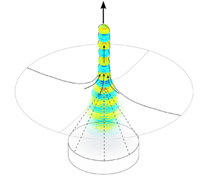
  $\varGamma _{exc}$. An illustration of the configuration for the acoustic fountain is given in figure 1. The expansions of pressure, velocity and density can be written as follows: $p=p_0 + p_1 + p_2, \boldsymbol {v}=\boldsymbol {v}_0 + \boldsymbol {v}_1 + \boldsymbol {v}_2, \rho =\rho _0 + \rho _1 + \rho _2$, respectively, to obtain the first-order acoustic equations defined in $\varOmega$,
 \begin{gather} \frac{1}{c_0^2} \partial_t p_1 + \rho_0 \boldsymbol{\nabla} \boldsymbol{\cdot} \boldsymbol{v}_1 = 0 , \end{gather}
 \begin{gather}\rho_0 \partial_t \boldsymbol{v}_1 ={-} \boldsymbol{\nabla} p_1 , \end{gather}
 \begin{gather}\rho_1 = \frac{1}{c_0^2}p_1 , \end{gather}
where  $c_0$ is the speed of sound in the liquid, assumed to be homogeneous. The static values for velocity and pressure were chosen to equal zero: $\boldsymbol {v}_0=\boldsymbol {0}, p_0=0$. A pure standing wave is assumed, and thus the acoustic equations can be transposed in the frequency-domain, leading to the Helmholtz equation for the acoustic pressure $p_1$,
 \begin{equation} \frac{1}{\rho_0}\nabla^2 p_1 + \frac{\omega^2}{\rho_0 c_0^2} p_1 =0 \ \text{in} \ \varOmega , \end{equation}
for a given driving pulsation  $\omega$ (in rad s $^{-1}$). One can define the acoustic wavenumber $k_0 = \omega /c_0$ and the acoustic wavelength $\lambda =(2{\rm \pi} )/k_0$. The acoustic pressure is assumed to be zero at $\varGamma _{free}$, i.e. the free surface can vibrate freely. As a consequence of this, only pure acoustic standing waves are considered and capillary standing waves are neglected (in this configuration, the vibration amplitude of a linear capillary wave is negligible). To represent the excitation of the transducer a normal vibration amplitude $u_{1,exc}$ is defined at $\varGamma _{exc}$, and at the rigid walls $\varGamma _{walls}$ the normal vibration amplitude is set to zero. The boundary conditions for the standing acoustic wave computation are summarised as follows:
 \begin{gather} p_1 =0 \ \text{at} \ \varGamma_{free} , \end{gather}
 \begin{gather}\boldsymbol{\nabla} p_1 \boldsymbol{\cdot} \boldsymbol{n} ={-} \rho_0 \omega^2 u_{1,exc} \ \text{at} \ \varGamma_{exc} , \end{gather}
 \begin{gather}\boldsymbol{\nabla} p_1 \boldsymbol{\cdot} \boldsymbol{n} = 0 \ \text{at} \ \varGamma_{walls} . \end{gather}
Figure 1. Representation of the axisymmetric FEM configuration for the acoustic fountain simulations. (a) Summary of the FEM geometry and view of the initial acoustic pressure. The domain's boundary is divided into the symmetry axis  $\varGamma _{axi}$, the free surface $\varGamma _{free}$, the rigid walls $\varGamma _{walls}$ and the transducer $\varGamma _{exc}$. The contour plot depicts the normalised acoustic pressure for an excitation of 1 MHz at $\varGamma _{exc}$. The normalisation is done with respect to the maximum absolute pressure of the field. (b) Overview of the computational mesh for an initial flat surface and a deformed surface.
The acoustic radiation force to compute the induced motion of the liquid is derived from the Helmholtz equation solution, and the second-order flow is assumed to be potential-irrotational,
 \begin{equation} \boldsymbol{v}_2= \boldsymbol{\nabla} \phi_2 \ \text{in} \ \varOmega , \end{equation}
for a scalar potential  $\phi _2$. The balance between surface tension and acoustic radiation pressure can be directly expressed at the free surface, applying the perturbation expansion method, as a boundary condition,
 \begin{equation} \rho_0 \partial_t \phi_2= \gamma \kappa - \tfrac{1}{2}\rho_0\langle ( \boldsymbol{\nabla} \phi_1 )^2 \rangle\ \text{at} \ \varGamma_{free} , \end{equation}
where  $\gamma$ is the surface tension and $\kappa$ is the curvature of the surface. The acoustic velocity potential $\phi _1$ is directly derived from the acoustic pressure: $\rho _0 \partial _t \phi _1=-p_1$. The $\langle {\cdot }\rangle$ notation denotes time averaging. As a pure standing wave is considered, the acoustic field is assumed to have the form $p_1(x,t)=p_1(x)\sin (\omega t)$ for the considered time period (usually several acoustic periods), so that the terms in $\langle \sin ^2(\omega t)\rangle$ and $\langle \cos ^2(\omega t)\rangle$ introduce a factor of $1/2$ when evaluating the time average, see e.g. Pavlic & Dual (Reference Pavlic and Dual2021). This formulation follows the common derivation from the Bernoulli equation (inviscid case) applied to the free surface of the liquid, see Galtier (Reference Galtier2021). Thus, in the configuration for which the liquid can be described as inviscid, the liquid motion caused by acoustic streaming is negligible compared with the motion of the free surface caused by the acoustic radiation force. The second term on the right-hand side of (2.9) can be called the average acoustic kinetic energy, from which the acoustic radiation force at the free surface is derived. Considering an inviscid and incompressible liquid, this leads to the following system of equations to calculate the average second-order motion:
 \begin{gather} \nabla^2 p_2 = 0 \ \text{in} \ \varOmega , \end{gather}
 \begin{gather}\rho_0 \partial_t \boldsymbol{v}_2 ={-}\boldsymbol{\nabla} p_2 \ \text{in} \ \varOmega , \end{gather}
 \begin{gather}p_2= \gamma \kappa - \tfrac{1}{2}\rho_0\langle ( \boldsymbol{\nabla} \phi_1 )^2 \rangle\ \text{at} \varGamma_{free} , \end{gather}
 \begin{gather}\boldsymbol{\nabla} p_2 \boldsymbol{\cdot} \boldsymbol{n} = 0 \ \text{at} \ \varGamma_{walls} \ \text{and} \varGamma_{exc}. \end{gather}
One can demonstrate that this formulation is equivalent to the general volume acoustic radiation force formulation involving the volume source term  $\mathcal {F}=-\rho _0 \boldsymbol {\nabla } \boldsymbol {\cdot } \langle \boldsymbol {v}_1 \otimes \boldsymbol {v}_1 \rangle$ (see Baudoin & Thomas Reference Baudoin and Thomas2020, p. 210) applied to the case of a free surface. The two systems for the first- and second-order motions were solved numerically using MATLAB R2021a. The numerical computation uses the following procedure:
(i) the standing acoustic field is computed from (2.4)–(2.7), with a FEM solver;
(ii) the interface curvature and acoustic radiation pressure are computed and set as Dirichlet boundary conditions at the free surface following (2.12);
(iii) $p_2$ is computed using a FEM solver for (2.10)–(2.13);
(iv)
$\boldsymbol {\nabla } p_2$ is computed using FEM gradient computation;(v) the Lagrangian motion of the free surface is computed by integrating equation (2.11) at the free surface using the forward Euler scheme;
(vi) the domain is remeshed according to the new boundary geometry defined by the free surface motion;
(vii) the velocity of the free surface is linearly interpolated on the new mesh;
(viii) the algorithm returns to the standing acoustic field computation to update the acoustic field for the new geometry.


The numerical Lagrangian motion of the free surface is similar to a ‘surface evolver’ approach, see Brakke (Reference Brakke1992) and Carter (Reference Carter1996), which consists of computing the motion of the nodes in the surface normal direction, remeshing of the surface to avoid distorted meshes, explicit integration of the surface tension and volume conservation constraints. The main benefit of our developed approach is that the acoustic radiation force and the surface tension is implemented in a consistent manner with the tracked and meshed surface. Contrary to Eulerian phase-field methods, there is no need for a surface reconstruction algorithm. On the other hand, the drawbacks are the time consumption in the remeshing procedure and the possible aberration when interpolating velocity from one mesh to another. Due to the relatively short duration of the phenomena and the relatively low absorption of the medium, heating up effects due to viscous dissipation were neglected, i.e. the temperature was assumed to be constant in the entire simulation domain.
2.2. Acoustic resonance
The FEM discretisation of the Helmholtz equation (2.4) leads to the following linear algebra formulation:
 \begin{equation} -\omega^2\boldsymbol{M}\boldsymbol{p}_1 + \boldsymbol{K}\boldsymbol{p}_1 = \boldsymbol{f} , \end{equation}
where  $\boldsymbol {M}$ is the mass matrix, $\boldsymbol {K}$ is the stiffness matrix, $\boldsymbol {p}_1$ is the unknown acoustic pressure vector and $\boldsymbol {f}$ is the excitation vector. The unknown acoustic pressure vector is then obtained by direct matrix inversion,
 \begin{equation} \boldsymbol{p}_1=[-\omega^2\boldsymbol{M} + \boldsymbol{K}]^{{-}1} \boldsymbol{f} . \end{equation}
The solution becomes singular for the following condition for any vector  $\boldsymbol {q}$:
 \begin{equation} [-\omega^2\boldsymbol{M} + \boldsymbol{K}] \boldsymbol{q}=\boldsymbol{0}. \end{equation}
This equation represents the eigenproblem associated with the matrix  $\boldsymbol {M}^{-1}\boldsymbol {K}$. In other words, the solution becomes singular if the excitation frequency matches an eigenfrequency of the current configuration. Modal decomposition, see e.g. Ewins (Reference Ewins2009, pp. 47–57), leads to the following formulation highlighting resonance in the solution:
 \begin{equation} \boldsymbol{p}_1=\left[\sum_{k=1}^{N} \frac{\boldsymbol{A}_k}{(\omega^2 - \omega_k^2)} \right]\boldsymbol{f} , \end{equation}
where  $N$ depends on the dimension of the discretised problem, $\boldsymbol {A}_k$ are the modal matrices associated with eigenmodes of indexes $k$. The acoustic pressure is proportional to the excitation, and becomes large when the excitation frequency $\omega$ approaches an eigenfrequency $\omega _k$. The resonance also induces a phase shift, a change in sign, when resonance is matched. The excitation of a particular mode is dependent on the relation of the distribution of the excitation in space and the mode pattern, through the product $\boldsymbol {A}_k \boldsymbol {f}$, corresponding to a modal projection. The absorption due to the liquid viscosity was defined as its theoretical value for water at the selected frequency. The characteristic relaxation time $\tau$ of a fluid is
 \begin{equation} \tau = \frac{\mu_b + \frac{4}{3}\mu}{\rho_0 c_0^2} , \end{equation}
where  $\mu _b$ is the bulk viscosity, and $\mu$ is the shear viscosity of the fluid. Using the viscosity values in table 1, the relaxation time $\tau$ for water at 20 $\,^\circ$C is $1.689\times 10^{-12}$ s. The equivalent loss factor damping model was implemented, which adds an imaginary part to the real stiffness matrix $\boldsymbol {K}'$,
 \begin{equation} \boldsymbol{K}=\boldsymbol{K}' + i \eta \boldsymbol{K}', \end{equation}
where  $\eta =\tau \omega$ is the loss factor, which equals $1.06\times 10^{-5}$ at 1 MHz. Taking the imaginary part of the wavenumber $k_0'=\omega /(c_0 \sqrt {1-i \omega \tau })$, one can show that this model gives an equivalent absorption coefficient of 0.0225 Np m $^{-1}$, or equivalently 0.002 dB cm $^{-1}$, which is consistent with commonly observed ultrasound absorption values in water at 1 MHz. Due to this relatively low absorption value the dampening term $i \eta \boldsymbol {K}'$ has limited impact on the acoustic field for the case of water.
Table 1. Fluid properties implemented in the numerical model.

2.3. Acoustic fountain configuration
For the numerical acoustic fountain study we reproduced the experimental set-up of Simon et al. (Reference Simon, Sapozhnikov, Khokhlova, Crum and Bailey2015) at an excitation frequency of 1 MHz and for different transducer excitation amplitudes. The associated acoustic wavelength  $\lambda$ is 1.48 mm. The tank was 80 mm in diameter and its height was set to 55 mm. The transducer was a spherical bowl shape transducer with an aperture of 45 mm, and it was placed at a distance of 45 mm from the free surface so that its location coincided with the geometric focus of the transducer. The fluid properties implemented in the numerical model are listed in table 1. The fluid is assumed to be at a constant temperature of 20 $\,^\circ$C and at atmospheric pressure, and all fluid properties were evaluated for this temperature and static pressure. Absorbing boundaries were set in the vicinity of the rigid walls to avoid possible spurious reflection of acoustic waves. The focused acoustic pressure field for the initial state is depicted in figure 1(a). An axisymmetric version of the model was used, with the following boundary condition at the axis: $\boldsymbol {\nabla } p_1 \boldsymbol {\cdot } \boldsymbol {n} = 0, \boldsymbol {\nabla } p_2 \boldsymbol {\cdot } \boldsymbol {n} = 0 \ \text {at} \ \varGamma _{axis}$. The computational mesh is depicted in figure 1(b). Linear triangle elements with three integration points were used, and the average cell size in the domain was set to $2\times 10^{-4}$ m. At the free surface, the mesh was refined to a cell size of $4\times 10^{-5}$ m. To reduce the remeshing time only a deformable region was remeshed, which was defined as a layer of 5 mm depth with respect to the initial free surface height. The solver follows the steps described in § 2.1 with an integration time step of $3\times 10^{-6}$ s, which is equal to three acoustic periods. The computation of the axisymmetric curvature $\kappa$ is given explicitly by
 \begin{gather} \kappa = \chi_1 + \chi_2 , \end{gather}
 \begin{gather}\chi_1 = \frac{r' z''-z'r''}{(r'^2 + z'^2 )^{3/2}}, \end{gather}
 \begin{gather}\chi_1 = \frac{ z'}{r(r'^2 + z'^2 )^{1/2}}, \end{gather}
where  $(r(s),z(s))$ are the parametric coordinates of the axisymmetric surface. The FEM inversion of the axisymmetric Laplacian in (2.10), as well as the FEM gradient computation in (2.11), introduces a singular behaviour near the axis that may cause a numerical aberration in this region, such as a non-physical velocity or breakup of the mesh due to too strong deformation. To smoothen the solution near the symmetry axis the radial coordinate was offset when constructing the numerical axisymmetric Laplacian: $r_{reg} = r + \epsilon$. This regularisation offset was set empirically to $\epsilon =3\times 10^{-4}$ m. The validation of the axisymmetric solver, especially the validation of the surface tension implementation, was performed with the free oscillating droplet benchmark. A relative error for the frequency of the fundamental droplet vibration mode of 1.17 % was obtained. The detailed result of the benchmark is given in the Appendix A.
An illustration of the change in the acoustic field pattern upon surface deformation is provided in figures 2(a) and 2(b), which depicts shadowgraph results reported in Tomita (Reference Tomita2014). The initial field in figures 2(a) and 2(d) consists of a focused beam. It is possible to show that the initial field at the free surface has a Bessel-beam pattern (see the Appendix B). As shown in figures 2(b) and 2(e), the initial beam is altered by the deformation of the free surface. The altered pattern shows interference lobes, due to the new reflecting geometry. The localised deformation forms a geometric focus for the acoustic waves. The shadowgraph technique is unable to detect the pattern inside the deformed growing region, but it is expected that the acoustic field is focused in this region as in figure 2(e).

Figure 2. Illustration of the acoustic field pattern upon surface deformation in an acoustic fountain experiment with a 1 MHz transducer focused at 80 mm from the surface. (a–c) Shadowgraphs taken at (a) 60  $\mathrm {\mu }$s and (b) 4.5 ms. Standing waves may be seen in the water layer in both (a) and (b), and an ejecting jet may be seen in (b). The acoustic intensity was 220 W cm $^{-2}$ and the exposure time 1000 ms. Here WS denotes the water surface. The scale bars represent 5 mm. (c) The onset time, $T_{ex,e}$, of the water surface elevation plotted as a function of the acoustic intensity, $I$. Reprinted from Y. Tomita, ‘Jet atomization and cavitation induced by interactions between focused ultrasound and a water surface’, Physics of Fluids 26, 097105 (2014), with the permission of AIP Publishing. (d,e) Qualitative comparison with obtained numerical results. (d) Initial acoustic field. (e) Predicted acoustic field after 10.2 ms.
3. Results
3.1. Solution types and transient bump analysis
The parameters of the different acoustic fountain simulations for an excitation frequency of 1 MHz are summarised in table 2. The main parameter is the excitation magnitude which can be either expressed in terms of that transducer normal vibration amplitude (boundary condition) or in terms of the initial pressure. The initial acoustic pressure is taken at the focus near the surface when the surface is at rest. It should be mentioned that these acoustic pressure values cannot be compared in an absolute way to the values reported in Simon et al. (Reference Simon, Sapozhnikov, Khokhlova, Crum and Bailey2015), which were measured inside the water tank and not near the surface where reflection occurs. A movie corresponding to each excitation magnitude is also provided in the Supplementary movies, which are available at https://doi.org/10.1017/jfm.2023.968 associated with this article. From the simulation results three different solution types can be identified. (i) At low excitation magnitudes (Magnitude 1 to 8) the acoustic radiation force is not sufficient to support the continuous growth of the liquid surface. Instead, uneven surface oscillations are observed resulting from the balance between the dynamic acoustic force and surface tension. (ii) At large excitation magnitudes (Magnitude 11 to 13) the acoustic radiation force almost immediately produces the acoustic fountain, which is triggered within a time period shorter than 10 ms. (iii) The intermediate solution type is the delayed fountain, triggered for times greater than 10 ms (Magnitudes 9 and 10). The initial behaviour for all solutions is similar as the formation of a transient bump is observed, as indicated in figure 3 which depicts the height of the deformed liquid surface in the centre ( $r=0$) for each simulation for a period of 10 ms. In the case of the surface oscillation solutions (Magnitude 1 to 8) the liquid height decreases again due to surface tension and inertia. For the immediate fountain solutions (Magnitude 11 to 13) the transient bump is followed by a further rapid increase of the liquid height. The predicted values for the surface height and the maximum velocity of the transient bump are provided in table 2.
Table 2. Summary of the different acoustic fountain simulations for an excitation frequency of 1 MHz. The values 12 and 40 ms indicate the start of the acoustic fountain.


Figure 3. Height of the deformed liquid surface in the centre ( $r=0$) for the different excitation magnitudes. The marker for each curve corresponds to the transient bump height. The three immediate acoustic fountain solutions are indicated by a dashed line, the two delayed acoustic fountain solution are indicated by a dashed–dotted line.
Figure 4 shows how the relative acoustic pressure, defined as the ratio of the maximum and the initial acoustic pressure, varies with liquid height near the free surface. It is evident from this figure that the dynamic acoustic pressure decreases in the transient phase as the bump grows. This trend is observed for all excitation magnitudes in the transient bump region. For the acoustic fountain solutions, the acoustic pressure starts to increase towards the next resonance peak when the liquid height reaches  $\lambda /4$. This observed nonlinear behaviour can be captured by the following ordinary differential equation with initial values for the liquid height $h$,
$h$,
 \begin{gather} \rho_0 \frac{{\rm d}^2h}{{\rm d}t^2} - B \frac{1}{8}k_{0}^3 \gamma h + A\frac{1}{4\rho c_0^2} p_a^2 k_{0}\, f^2(h)H^2(t) =0 , \end{gather}
 \begin{gather}h(t=0)=0, \end{gather}
 \begin{gather}\frac{{\rm d}h}{{\rm d}t}(t=0)=0, \end{gather}
where  $p_a$ denotes the initial acoustic pressure, and $k_{0}$ the acoustic wavenumber ( $k_0 = 2{\rm \pi} /\lambda$). The first term represents inertia, the second surface tension and the third term the acoustic radiation force. The function $H(t)$ is the time envelope of the acoustic signal, in this study we selected a Heaviside step function. The non-dimensional parameters $A$ and $B$ are fitting parameters, and the dimensionless nonlinear parameter $f(h)$ represents the relative change of acoustic pressure with the liquid height. Here $f(h)$ can either be evaluated directly from the pattern in the transient bump region of figure 4 or by fitting the pattern with an empirical function. We noticed that the following expression:
 \begin{equation} f(h) = (1-b) e^{{-}a h} + b , \end{equation}
with  $a=1.1\times 10^4\ {\rm m}^-1$ and $b=0.4$, fits the pattern well (see the dashed line in figure 4). This enables us to integrate (3.1) for a given initial acoustic pressure and to fit the parameters $A$ and $B$ to the observed transient bump heights. The obtained fitting parameters were $A=1.186$ and $B=0.245$, and theresults of the fit are provided as dashed lines in figure 5 and compared with the numerically determined bump height, bump velocity and bump time subject to the transducer amplitude and the initial acoustic pressure. The results of the static acoustic field approximation, taking $f(h)=1$, with the same values of $A$ and $B$ are also plotted as dotted lines in figure 5. It is clear that the static approximation and its corresponding quadratic equations ( $h_{max}=0.2986\times 10^{-15}p_a^2$ and $\dot {h}_{max}=1.3224\times 10^{-13}p_a^2$ for the maximum height and velocity, respectively) is not able to capture the dynamics of the phenomenon.

Figure 4. Relative acoustic pressure (ratio of the maximum and the initial acoustic pressure) subject to the liquid height (evaluated in the centre  $r=0$) for all simulations. Each solid curve is associated with the corresponding simulation.

Figure 5. Analysis of the liquid deformation in the transient bump regime. (a) Liquid surface height in the centre ( $r=0$) when reaching the bump. (b) Maximum transient velocity in the centre ( $r=0$). (c) Time to reach the maximum bump height.
3.2. Analysis of the drop-chain fountain solution
Figure 6 highlights the dynamic acoustic field obtained for the Magnitude 11 case, for which the growing drop-chain is observed. The magnitude of the acoustic field is quantified via the absolute maximum values of the two fields: acoustic pressure  $p_1$ (in Pa) and acoustic particular oscillation amplitude $\boldsymbol {u}_1$ (in m, $\partial _t\boldsymbol {u}_1=\boldsymbol {v}_1$). The latter is obtained from a gradient computation of the acoustic pressure field according to (2.2). The first resonance peak occurs when the transient bump reaches a height of $\lambda /4$, and acts as the drop-chain starter. The second resonance peak is observed at around 9.5 ms, when the height of the liquid is close to $\lambda /2$. The apparent sudden drop in amplitude in the resonance peak corresponds to the typical ${\rm \pi}$ phase-shift, which is observed in the change of sign in the contour plots of the acoustic pressure field. For $t>10$ ms further resonance peaks are observed, which coincide with the drop-chain height reaching multiple values of $\lambda /4$. The typical peak amplitude is in the range of 5 MPa to 10 MPa (acoustic pressure) and 0.25 $\mathrm {\mu }$m to 0.60 $\mathrm {\mu }$m (acoustic vibration amplitude). Figure 7 depicts the instantaneous liquid velocity in the centre for the three immediate fountain solutions (Magnitude 11–13). These values can be put into perspective with the experimental observations of Simon et al. (Reference Simon, Sapozhnikov, Khokhlova, Crum and Bailey2015) (figure 7b) where an instantaneous growing speed in the range of 0.2 to 1.4 m s $^{-1}$ was observed. It can be seen in figure 7(a) that the Magnitude 12 case exhibits a strong instability with a growing velocity above 4 m s $^{-1}$, resulting in numerical divergence.

Figure 6. Dynamic acoustic field, given in terms of maximum absolute acoustic pressure and particular oscillation amplitude, for the Magnitude 11 simulation. Contour plots in normalised scale of the acoustic pressure are provided for different resonance peaks together with the associated vertical velocity. (a) Time period from 0 ms to 13 ms and (b) time period from 13 ms to 22 ms.

Figure 7. Comparison of the predicted drop-chain growing velocity with the experiments of Simon et al. (Reference Simon, Sapozhnikov, Khokhlova, Crum and Bailey2015). (a) Centre point velocity for the Magnitude 11–13 cases. (b) Drop-chain velocity extracted from the movie provided in Simon et al. (Reference Simon, Sapozhnikov, Khokhlova, Crum and Bailey2015) for an excitation frequency of 1 MHz.
3.3. Analysis of drop diameters
As shown in the previous section, the acoustic field forming the growing drop-chain solution consists of a sequence of resonance peaks coinciding with a drop-chain height reaching multiple values of  $\lambda /4$. Consequently, a sequence of growing drops of even diameter is formed, which is a characteristic of this system. The drop diameters were extracted by automatic peak detection from the wavy shape over time, and figure 8 depicts the single drop diameter for the Magnitude 11 case. The first formed drop exhibits a diameter of approximately 1.4 mm which corresponds to $\approx 0.95\lambda$. Between 10 to 22 ms a drop chain of even diameters of around $\lambda$ is formed. The acoustic shock at around 23.6 ms produces a sudden deformation that breaks the regular distribution of the drop diameter, resulting in a complex deformation pattern.

Figure 8. Evolution of the drop diameter over time for the Magnitude 11 case. The drop diameter is normalised with respect to the acoustic wavelength  $\lambda$.
3.4. Atomisation at the surface of the acoustic fountain
The acoustic field intensity can be analysed with respect to the atomisation threshold for the given liquid and driving frequency (1 MHz) to predict when and where the acoustic fountain atomises. Considering pure Faraday-instability atomisation, there are two different thresholds: (i) the Faraday threshold, at which a standing Faraday wave is formed at the surface of the liquid; and (ii) the atomisation threshold, at which the crests of the Faraday wave start to break to form droplets. The Faraday threshold was computed according to the Kumar & Tuckerman (Reference Kumar and Tuckerman1994) theory, the obtained critical Faraday wavelength is  $\lambda _{Faraday} = 12.12$ $\mathrm {\mu }$m and the critical vibration amplitude is $|u|_{Faraday} =0.266$ $\mathrm {\mu }$m. The average diameter of the ejected droplets is expected to be a fraction of $\lambda _{Faraday}$, generally around $0.35 \lambda _{Faraday}$ (Lang Reference Lang1962), corresponding to a diameter of around 4.2 $\mathrm {\mu }$m. However, the droplet size distribution can be broad due to the formation of child droplets from ligaments, the mist effect and coalescence, see e.g. Barreras et al. (Reference Barreras, Amaveda and Lozano2002), Kudo et al. (Reference Kudo, Sekiguchi, Sankoda, Namiki and Nii2017), Kooij et al. (Reference Kooij, Astefanei, Corthals and Bonn2019), Zhang, Yuan & Wang (Reference Zhang, Yuan and Wang2021) and Zhang, Yuan & Gao (Reference Zhang, Yuan and Gao2023). To estimate the atomisation threshold we performed volume of fluid (VOF) simulations as described in our previous work (Cailly et al. Reference Cailly, Mc Carogher, Bolze, Yin and Kuhn2023), and additional details are provided in the Appendix C. Atomisation is defined at the point where breakup is observed for a free surface vibrating at a given driving amplitude and frequency, and the obtained atomisation threshold is $|u|_{atomisation,VOF} = 1.1$ $\mathrm {\mu }$m. As discussed above, a sudden large amplitude resonance peak occurs at 23.5 $\mathrm {\mu }$s for the Magnitude 11 case, see also figure 9(a). The oscillation amplitude of this peak is larger than the Faraday threshold, i.e. Faraday waves are excited on the liquid surface. The fraction of the peak above the VOF-predicted atomisation threshold corresponds to an atomisation burst consisting of a jet of ejected droplets. For this particular atomisation event the duration of the burst is around 35 $\mathrm {\mu }$s. Figure 9(b) depicts the vibration pattern at $t=23.62$ ms corresponding to the largest acoustic intensity. It is observed that the acoustic vibration pattern is not homogeneous along the drop-chain. The arrows in figure 9(b) correspond to the acoustic vibration vector, given in norm representation since the instability is independent of the sign of the vibration, allowing us to identify the loci of atomisation events. Figures 10(c) and 10(d) represent atomisation burst patterns as recorded by Simon et al. (Reference Simon, Sapozhnikov, Khokhlova, Crum and Bailey2015). In these experimental images an axisymmetric ‘ring shape’ atomisation pattern is observed, with atomisation events at specific vertical positions and at the top of the drop-chain (figure 10d).

Figure 9. An atomisation burst produced by an acoustic-resonance shock. The numerical results are taken from the Magnitude 11 case, and the images are extracted from the movie provided in Simon et al. (Reference Simon, Sapozhnikov, Khokhlova, Crum and Bailey2015) for an excitation frequency of 1 MHz. (a) Absolute acoustic pressure and particular oscillation amplitude compared with the Faraday ( $|u|_{Faraday}$) and estimated ( $|u|_{atomisation,VOF}$) atomisation threshold. (b) Predicted atomisation burst pattern. (c) Image showing a typical atomisation burst pattern. (d) Image showing a typical atomisation burst pattern – obtained at a different time than (c).

Figure 10. The flattened drop shape due to an acoustic resonance shock. The numerical results are taken from the Magnitude 11 case, and the images are extracted from the movie provided in Simon et al. (Reference Simon, Sapozhnikov, Khokhlova, Crum and Bailey2015) for an excitation frequency of 1 MHz. (a) Acoustic pressure field at  $t=23.6$ ms, the arrows represent the acoustic radiation force at the free surface. (b) Deformed shape after 1 ms. (c) Image of a growing drop-chain. (d) Image of a transient deformation pattern of the same drop-chain (c) after 1.4 ms. The highlighted liquid border was added to the original images.
Another consequence of a sudden large amplitude resonance peak is the relatively large deformation of the drop-chain fountain that follows the peak. This phenomenon is illustrated in figure 10(a), which depicts the acoustic force pattern at  $t=23.6$ ms, associated with the previously discussed resonance peak. During the resonance peak period the acoustic force dominates surface tension, leading to strong interface deformation by alternately pushing the liquid outwards and pulling the liquid towards the centre, corresponding to the acoustic field pattern. As a consequence, spherical drops are deformed into flattened drops. This is exemplified in figure 10(b) which shows the deformed liquid after 1 ms and where flattened drops are observed in the locations of largest acoustic force. These predictions agree with the experimental observations by Simon et al. (Reference Simon, Sapozhnikov, Khokhlova, Crum and Bailey2015). The images in figures 10(c) and 10(d) depict the evolution of an atomisation burst pattern over a time period of 1.4 ms. The acoustic force results in a strong localised deformation flattening the second droplet from the bottom. The deformation is so strong that breakup of the drop-chain is observed. The top droplet in figure 10(c) was subjected to the same phenomenon (see complete result in Simon et al. (Reference Simon, Sapozhnikov, Khokhlova, Crum and Bailey2015)).
4. Discussion
The aim of this work is to contribute to an improved understanding and description of the acoustic deformation of a liquid irradiated by ultrasound. The developed numerical approach is able to capture the mechanism of the acoustic fountain, and a good qualitative agreement with experiments is observed. Depending on the excitation magnitude, different regimes are found, which highlights the sensitivity of the acoustic fountain behaviour to the input magnitude. This observation is also in line with experiments as this sensitivity is found by comparing the shapes for different excitations in Tomita (Reference Tomita2014, p. 097105-4). Furthermore, the growing drop-chain solution is also numerically well reproduced, and for example, the Magnitude 11 case exhibited an even drop-chain behaviour. The shape of the base cone of the fountain (see e.g. figure 6b) is consistent with the typical shape observed in experiments. The analysis of the dynamic acoustic field allowed us to highlight the sequence of resonance peaks coinciding with drop formation. As reported by Wang et al. (Reference Wang, Mori and Tsuchiya2022) the expected drop diameter equals the acoustic wavelength in the liquid  $\lambda$, which is also predicted by our simulations for even drop-chain solutions.
Furthermore, a consistent order of magnitude of the growing velocity is predicted. In Simon et al. (Reference Simon, Sapozhnikov, Khokhlova, Crum and Bailey2015) an acceleration from 0.4 to 1.4 m s $^{-1}$ is observed. Similar acceleration patterns are observed in the simulations, for example, the resonance peak at $t=23$ ms in the Magnitude 11 simulation produces an acceleration from 0.25 to 1.78 m s $^{-1}$ (see figure 7a). Then, after the resonance peak, the growing velocity decreases to a value of approximately 1.2 m s $^{-1}$, leading to a pattern similar to the observation in Simon et al. (Reference Simon, Sapozhnikov, Khokhlova, Crum and Bailey2015). Wang et al. (Reference Wang, Mori and Tsuchiya2022, p. 5) measured the growing velocities in the range from 0.102 to 0.183 m s $^{-1}$, and Tomita (Reference Tomita2014, p. 097105-8) obtained an average growing velocity of 2.1 m s $^{-1}$. The presented numerical approach demonstrates how the growing velocity fluctuates due to the complexity of the dynamic acoustic field and to surface tension counteracting the growth. For the acoustic fountain solutions, the predicted values are in the range from 0.1 m s $^{-1}$ to 2.0 m s $^{-1}$, which is consistent with the associated acoustic pressures. A strong resonance peak can also produce a sudden acceleration of the fountain. The complex deformation regime consisting of constrictions and large droplets, as observed by Wang et al. (Reference Wang, Mori and Tsuchiya2022, p. 5) at a power density of 7 W m $^{-2}$ and a frequency of 3.0 MHz, is a consequence of a briefly acting strong acoustic force. For a relatively high acoustic intensity, the liquid velocity can exceed 4 m s $^{-1}$, and a complex unstable behaviour is observed. For these high intensities the developed model reaches its limitation, for example for the Magnitude 12 case too large deformations, resulting from numerical aberration, with a radial expansion above 4 mm are observed. For these cases the breakup of the liquid is expected, which is, however, not implemented in the developed numerical method. This type of primary breakup has been reported by Simon et al. (Reference Simon, Sapozhnikov, Khokhlova, Wang, Crum and Bailey2012, p. 8069) and Tomita (Reference Tomita2014, p. 097105-4). It has to be noted that a relatively smooth wavy shape is observed instead of a clear drop-chain with thin constrictions, which is due to the radial regularisation necessary to prevent aberration and early breakup near the axis (see § 2.3).
The quantitative analysis of the transient bump regime demonstrated the effect of the nonlinearity associated with the liquid deformation. The quadratic relation between transducer excitation amplitude and the liquid deformation, derived from the static acoustic field approximation, leads to a significant deviation. We showed that a simple model taking into account the loss of the acoustic field amplitude due to a resonance peak transition, provides a good description of the liquid deformation. The introduced nonlinearity factor will depend on the configuration. This result, summarised in figure 5, shows how the observation of liquid deformation can be used to characterise the ultrasonic excitation. There is a one-to-one deterministic relation between the ultrasonic excitation and the liquid deformation amplitude and velocity. However, as demonstrated in figure 5(c), there is no one-to-one relation between the time delay to reach the deformation and the excitation amplitude. Thus, it makes it difficult to characterise the ultrasonic excitation using this delay. We noticed that the nonlinear trend observed in figure 5(c) is similar to the one measured by Tomita (Reference Tomita2014, p. 097105-3), depicted in figure 2(c), where a delay of 2 ms is found compared with the 2.5 ms predicted in our numerical study. The delay measured by Tomita (Reference Tomita2014) was defined as the onset of the continuously growing acoustic fountain, corresponding roughly to our the definition of the transient bump phase.
The computation of the dynamic acoustic field in the acoustic fountain also allowed us to predict atomisation. As observed in the Magnitude 11 case, atomisation can be directly linked due to an acoustic resonance peak. As the Faraday instability arises, strong acoustic oscillations occur on specific locations of the growing surface, giving rise to specific atomisation burst patterns. A microdroplet generation time of approximately 30  $\mathrm {\mu }$s corresponds to the time span of the resonance peak above the atomisation threshold. It is observed that most of the resonance peaks are below the atomisation threshold, and that peaks above the atomisation threshold arise for a very specific deformation of the resonating liquid, implying that atomisation bursts only arise sporadically. A consequence of the sudden high amplitude acoustic shock is that local atomisation is associated with a strong local deformation of the liquid. The link between atomisation bursts and acoustic deformation was also observed experimentally by Simon et al. (Reference Simon, Sapozhnikov, Khokhlova, Crum and Bailey2015) and Wang et al. (Reference Wang, Mori and Tsuchiya2022). Furthermore, Cailly et al. (Reference Cailly, Mc Carogher, Bolze, Yin and Kuhn2023) found that in sonicated gas–liquid segmented flow atomisation coincides with a strong concave deformation of a bubble. Therefore, we conclude that dynamic acoustic resonance is the main mechanism driving both the drop-chain growth of the liquid and atomisation.
A distinction has to be made between Faraday-instability atomisation and cavitation-driven atomisation. The effect of cavitation bubbles is not directly predicted by the presented model as the acoustic field is computed neglecting any cavitation activity in the liquid. Cavitation is also expected to be less dominant at the selected high ultrasound driving frequency compared with the low frequency range, for which attenuation and nonlinear effects arise, see e.g. Louisnard & Garcia-Vargas (Reference Louisnard and Garcia-Vargas2022). Nevertheless, considering the computed acoustic pressure magnitude at the resonance peaks, which can reach tens of megapascals at 1 MHz, cavitation can still be expected. For these high pressure resonance peaks large cavitation bubbles (super-resonant cavitation bubbles) could be generated. Large cavitation bubbles inside the acoustic fountain together with Faraday atomisation were observed by Simon et al. (Reference Simon, Sapozhnikov, Khokhlova, Wang, Crum and Bailey2012, pp. 8068–8069), Simon et al. (Reference Simon, Sapozhnikov, Khokhlova, Crum and Bailey2015, p. 136) and by Tomita (Reference Tomita2014, p. 097105-8). The predicted acoustic pressure in the acoustic fountain can be related to experimental cavitation thresholds, obtained in almost similar conditions, to describe these observations. Herbert, Balibar & Caupin (Reference Herbert, Balibar and Caupin2006) measured the cavitation threshold at 1 MHz in distilled degassed water at different temperatures. At 20 $\,^\circ$C the cavitation pressure is in the range from 16 MPa to 30 MPa (Herbert et al. Reference Herbert, Balibar and Caupin2006, p. 041603–4), and it is found to decrease monotonically with temperature: from 26 MPa at 0.1 $\,^\circ$C to 17 MPa at 80 $\,^\circ$C. Furthermore, the authors highlight the importance of water purity, as the cavitation threshold varies largely depending on impurities and gas content. A similar experimental study using a 1 MHz focused transducer was carried out by Vlaisavljevich et al. (Reference Vlaisavljevich2016), in which the decrease of cavitation pressure with temperature was confirmed: from 29.8 MPa at 10 $\,^\circ$C to 14.9 MPa at 90 $\,^\circ$C. Figure 11 summarises the different acoustic pressure thresholds for water at 1 MHz as a function of temperature, allowing us to distinguish the different phenomena. The atomisation VOF and Faraday instability curves were computed using the Kumar & Tuckerman (Reference Kumar and Tuckerman1994) method and the modified Goodridge formula using a value of 0.9 for the constant (see the Appendix C), respectively. For this, the temperature dependence of surface tension, density, speed of sound and shear viscosity was implemented using the values reported in Vlaisavljevich et al. (Reference Vlaisavljevich2016, p. 1066). The Faraday instability and atomisation thresholds were converted into an acoustic pressure using the relation between the particular oscillation $u$ (in m) and the acoustic pressure (in Pa) from (2.2). Based on the works of Herbert et al. (Reference Herbert, Balibar and Caupin2006) and Vlaisavljevich et al. (Reference Vlaisavljevich2016) the cavitation threshold of water at 1 MHz is in the range of 24–28 MPa at 20 $\,^\circ$C. As a consequence, cavitation bubbles should appear during a resonance peak. The strong peak obtained for the Magnitude 11 simulation (see figure 9a), has an acoustic pressure above 25 MPa. The short time period of approximately 50 $\mathrm {\mu }$s is sufficient for a cavitation bubble to expand. According to Vlaisavljevich et al. (Reference Vlaisavljevich2016) the bubble growth time is estimated to be 10 $\mathrm {\mu }$s to 30 $\mathrm {\mu }$s, for diameters from 300 $\mathrm {\mu }$m to 500 $\mathrm {\mu }$m. This was confirmed by optical images where large cavitation bubbles of approximately 300 $\mathrm {\mu }$m in diameter were observed. Tomita (Reference Tomita2014) observed a bubble growing time of approximately 20 $\mathrm {\mu }$s and a sustain time during which the bubble is visible of 40 to 50 $\mathrm {\mu }$s. The maximum diameter of the visible bubble was approximately 200 $\mathrm {\mu }$m. Simon et al. (Reference Simon, Sapozhnikov, Khokhlova, Wang, Crum and Bailey2012) observed bubble diameters from 120 $\mathrm {\mu }$m up to 600 $\mathrm {\mu }$m. One can speculate that for sufficiently large acoustic pressures (above 30 MPa at 20 $\,^\circ$C) cavitation and Faraday atomisation coexist. It is known that large cavitation bubbles are moved to pressure nodes by the acoustic radiation force (Mc Carogher et al. Reference Mc Carogher, Dong, Stephens, Leblebici, Mettin and Kuhn2021), and in the case of the acoustic fountain the free surface acts as a pressure node. The phenomenon of a large cavitation bubble penetrating the interface was observed experimentally. Simon et al. (Reference Simon, Sapozhnikov, Khokhlova, Crum and Bailey2015) observed a complex cavitation-driven atomisation due to the generation of a set of large bubbles. From a pure deterministic point of view, unlike the atomisation burst due to a strong Faraday instability at a resonance peak, jets generated by cavitation bubbles appear to be more isolated and unpredictable.

Figure 11. Cavitation and atomisation thresholds for water at 1 MHz as a function of temperature. For cavitation, the acoustic pressure value corresponds to a negative peak. The values of acoustic pressure at 20 $\,^\circ$C are given.
5. Conclusion
A numerical approach based on the perturbation expansion method and an adaptive Lagrangian solver allowed us to accurately reproduce the acoustic fountain effect. The role of the dynamic acoustic field in this nonlinear system is demonstrated, and the analysis of the predicted acoustic field provides a novel understanding of this phenomena. As the liquid surface grows, the acoustic field is characterised by high intensity peaks, corresponding to the acoustic resonance effect. These resonance peaks also lead to the formation of droplets with a diameter equalling the acoustic wavelength. The large transient deformations of the liquid surface and atomisation bursts are also the direct consequence of these strong acoustic resonance peaks. Furthermore, the predicted acoustic pressure during these strong peaks can exceed the cavitation threshold. Despite the fact that cavitation appears to be more isolated and unpredictable in such systems, the results allow the prediction of the generation of super-resonant cavitation bubbles, consistent with previous experimental observations. The presented results also indicate the coexistence of cavitation and atomisation in acoustic fountains involving large acoustic pressures. The limits of the modelling approach were identified for strong and chaotic deformations which include breakup and combined atomisation and cavitation.
Supplementary movies
Supplementary movies are available at https://doi.org/10.1017/jfm.2023.968. Supplementary movies are made available with this article, where Movie $N$.mp4 corresponds to the Magnitude $N$ simulation. One frame corresponds to eight integration steps. The upper part shows the shape of the moving liquid surface. The vertical velocity in the centre of the fountain is displayed and the colour scale characterises the acoustic vibration with respect to the following thresholds: light blue, below the Faraday threshold; red, above the Faraday threshold and below the atomisation threshold; orange, above the atomisation threshold. The lower part shows the evolution of the maximum absolute pressure over time.
Funding
The authors acknowledge funding from the European Research Council (ERC) under the European Union's Horizon 2020 research and innovation programme (grant agreement no. 101001024) and the Research Foundation Flanders (G0B5921N).
Declaration of interests
The authors report no conflict of interest.
Appendix A. Validation of the axisymmetric solver for the free oscillation of a droplet
The assessment of the axisymmetric solver, described in § 2.1, was carried out considering the case of the free oscillation of a droplet. This dynamic system is characterised as a balance between inertia and surface tension. Consequently, this case enables us to validate the correct implementation of surface tension. The benchmark consisted of simulating the fundamental mode for which the shape and frequency are known analytically. The axisymmetric-mode frequencies of a droplet of radius  $R$ can be obtained from Lamb's formula (see e.g. Strani & Sabetta Reference Strani and Sabetta1984)
 \begin{equation} \omega^2_n=\frac{n(n-1)(n+1)(n+2)\gamma}{(n+1)\rho R^3} , \end{equation}
for  $n=2,3,4,\ldots$ . A water droplet ( $\rho =1000\ {\rm kg}\ {\rm m}^{-3}$, $\gamma =0.072\ {\rm N} {\rm m}^{-1}$) with a radius of 2 mm was considered. Initially, the droplet was given an elliptic shape with a radii ratio of 0.9. A constant volume constraint was applied in the calculation to ensure volume conservation for each time step (the integration time step was $1\times 10^{-4}$ s). The mesh size was $1.3\times 10^{-4}$ m, and the droplet's free surface was refined with a mesh size of $3.6\times 10^{-5}$ m. Figure 12(a) depicts the mesh in the initial state, and figures 12(b) and 12(c) show the result of the benchmark. The predicted oscillation frequency is 42.2 Hz. which results in a relative error of 1.17 % compared with the theoretical frequency of 42.7 Hz (see (A1)). As shown in figure 12(b), the ratio between the pole and the equator displacement was also well reproduced, due to the applied volume conservation the displacement is larger at the pole.

Figure 12. Results of the free oscillation of a droplet benchmark. (a) View of the initial mesh. (b) Droplet oscillation shape. (c) Displacement of the pole and equator points over time. The displacement is taken relatively to the equilibrium spherical shape. The dashed curves correspond to the theoretical linear solution.
Appendix B. Initial acoustic beam pattern at the free surface
The acoustic field at the free surface is depicted in figure 13. It is known that focused spherical transducers produce Bessel-beams. The obtained numerical field was compared with the ideal Bessel-beam in the radial direction, by fitting the result to the equation for the normalised acoustic velocity  $v_{z,a}$,
 \begin{equation} v_{z,a} (r)= \frac{J_1(k_r r)}{k_r r}, \end{equation}
where  $J_1$ is the Bessel function of the first kind of order $1$, and $k_r$ is the characteristic radial constant of the beam (in m $^{-1}$). The fit resulted in a value of $k_r = 2.05\times 10^3 \textrm {m}^{-1}$ and a corresponding $F$-number of 1.035 ( $F={\rm \pi} /(\lambda k_r)$). For an $F$-number close to 1 the focal distance coincides with the source diameter (Simon et al. Reference Simon, Sapozhnikov, Khokhlova, Crum and Bailey2015). The acoustic force at the free surface is calculated from the vertical acoustic velocity, see figure 13(b). Taking the force beam diameter at approximately half of the main lobe amplitude, it follows that the diameter of the pushed liquid corresponds to approximately the wavelength in the liquid $\lambda$. This is consistent with the general observation that the diameter of the liquid deformation is of the order of $\lambda$.

Figure 13. Comparison of the computed acoustic field at the free surface ( $\varGamma _{free}$) produced by a 1 MHz focused transducer in the initial state (flat surface) with the Bessel-beam approximation. (a) Normalised acoustic velocity $v_z/v_{z,r=0}$. (b) Normalised acoustic force $f_z/f_{z,ref}$. The normalisation of the acoustic force was done with respect to $f_{z,ref}=({\omega }/{c_0}){1}{4}\rho _0 v_{z,max}^2$. The vertical line $r=\lambda / 2$ allows us to compare the force lobe diameter with respect to the current wavelength.
Appendix C. The VOF simulations for estimating the atomisation threshold at 1 MHz
In this article, we defined the atomisation threshold as the free surface vibration amplitude at which breakup at the Faraday wave crests is observed. In our previous study on atomising liquid slugs in segmented flow, we showed that this threshold can be predicted by VOF simulations (Cailly et al. Reference Cailly, Mc Carogher, Bolze, Yin and Kuhn2023). A standard two-dimensional OpenFOAM solver interFoam modified according to Yin & Kuhn (Reference Yin and Kuhn2022) was used, and the detailed methodology is provided in Cailly et al. (Reference Cailly, Mc Carogher, Bolze, Yin and Kuhn2023). The method is consistent with the Kumar & Tuckerman (Reference Kumar and Tuckerman1994) theory for predicting the Faraday instability threshold at the selected frequency. The simulations were performed at a driving frequency of 1 MHz, and the domain consisted of a  $300 \times 300\ \mathrm {\mu }$m square. A vibration wall boundary condition was defined at the bottom and the Faraday wave generated at the free surface was predicted for different driving oscillation amplitudes. The results are illustrated in figure 14. For a vibration amplitude of 1.0 $\mathrm {\mu }$m no breakup is observed, contrary to a vibration amplitude of 1.1 $\mathrm {\mu }$m which showed breakup (observable at around 15 $\mathrm {\mu }$s). Thus, we assumed that below this value no atomisation is generated.

Figure 14. Estimation of the atomisation threshold at 1 MHz using OpenFOAM simulations. (a,b) Phase fraction at 15.7  $\mathrm {\mu }$s and 22.7 $\mathrm {\mu }$s for a 1.0 $\mathrm {\mu }$m driving oscillation amplitude. (c,d) Phase fraction at 15.7 $\mathrm {\mu }$s and 22.7 $\mathrm {\mu }$s for a 1.1 $\mathrm {\mu }$m driving oscillation amplitude.
We found that this method may be more relevant rather than directly applying the following Goodridge's formula (Goodridge et al. Reference Goodridge, Shi, Hentschel and Lathrop1997; Goodridge, Hentschel & Lathrop Reference Goodridge, Hentschel and Lathrop1999):
 \begin{equation} a_d \approx 0.26 \left(\frac{\gamma}{\rho_0}\right)^{1/3} \omega^{4/3} , \end{equation}
where  $a_d$ is the critical driving acceleration of the onset of drop ejection, vibration amplitude is computed with the relation $u_d=a_d/\omega ^2$, which we noticed it overestimates the atomisation at ultrasonic frequencies. Indeed, applying (C1) gives $u_d=0.5\ \mathrm {\mu }$m. As in Cailly et al. (Reference Cailly, Mc Carogher, Bolze, Yin and Kuhn2023), dealing with 500 kHz atomisation, we noticed that the VOF atomisation threshold is consistent with Goodridge's formula taking a constant of 0.9 instead of 0.26 in (C1).


