


The Dust Bowl of the 1930s was one of the greatest environmental and economic catastrophes in U.S. history. The severity of its environmental degradation, farm failure, and economic dislocation has cemented the episode’s place in the mythology of the American experience. Perhaps the most enduring image of the Dust Bowl is the exodus of destitute farmers and other “Okies” from the Southern Great Plains, one of the most famous episodes of internal migration in American history. However, scholars’ understanding of this migration episode has been limited by a lack of systematic data on affected individuals. This article uses newly constructed data to quantify and analyze gross migration flows associated with this event.
The Dust Bowl resulted from the confluence of drought, erosion, and economic depression throughout the Great Plains. The drought began in the winter of 1931; throughout most of the 1930s, and especially mid-decade, minimal precipitation, high winds, and pestilence led to widespread crop failure. While the effects were widespread, matters were most severe in the Southern Plains states of Colorado, Kansas, Oklahoma, and Texas (Joel Reference Joel1937; Cunfer Reference Cunfer2011), and the out-migration from this region looms largest in the formation of the Dust Bowl narrative.
Poor seasons were not new to the Plains in the 1930s. Yet in many ways the decade was unprecedented. One fundamental difference from previous droughts was the number of people affected. Between 1890 and 1930, according to the U.S. population censuses, the population of the Southern Plains states had increased from 4,496,000 to 11,561,000. Most striking was the severity of the drought, the worst in more than hundred years of formal meteorological record keeping.Footnote 1 Dust storms, like the famous Black Sunday storm of April 1935, were also more frequent and damaging. Severe wind erosion and occasional water erosion resulted in widespread loss of topsoil and declining agricultural productivity. These problems were exacerbated by the externalities associated with small-scale Plains agriculture, which dis-incentivized farmers from engaging in basic erosion prevention measures (Hansen and Libecap Reference Hansen and Libecap2004).
The environmental calamity coincided with the Great Depression. Together, these shocks amplified long-term structural change in agriculture, due to mechanization, consolidation, and falling agricultural prices since the end of WWI. Prices fell precipitously in the early 1930s, severely impacting farm incomes. Wheat prices fell from $1.18 per bushel in 1928 to 38 cents per bushel in 1932 and 1933; cotton prices fell from 19 cents to 6 cents per pound during the same period.Footnote 2 Falling incomes, coupled with farmers’ declining access to credit due to the financial sector crisis, led to foreclosure and farm loss.
As a result, the region experienced marked depopulation. During the Dust Bowl decade, populations in the most greatly affected counties shrank by 20 percent. Using county-level data, Richard Hornbeck (Reference Hornbeck2012) shows that population declined by 12 percent in the Great Plains counties that experienced the highest levels of erosion relative to counties with less erosion.Footnote 3 This trend was long lasting as the bulk of long-run reallocation of productive factors away from agriculture was achieved through population decline as opposed to adjustments in land use.
This displacement led to much public hand-wringing and anger in places receiving the “tide of migration … sweeping over the country” (see U.S. House of Representatives 1941, p. 68), and gave rise to derogatory terms such as “Okies” and “Dust Bowl refugees.” Perhaps the most vivid example is that of the Los Angeles Police sending officers to patrol the California borders to stem the immigration. Certainly, the “transient problem” was more general in scope, due to the joblessness created by the Great Depression. Still, the flight from the Dust Bowl clearly loomed large, both in the popular consciousness and in Congress, which in 1940 established a select committee to “investigate the interstate migration of destitute citizens.”
These factors came together to cement the Dust Bowl’s place in American myth, and to make the exodus from the Southern Great Plains one of the most famous episodes of internal migration in U.S. history. The Dust Bowl loomed large in literature, art, and music—from the iconic images of the Farm Security Administration photography corps documenting the plight of Plains farmers and its migrants, to the folk songs of Woody Guthrie, to films like Pare Lorentz’s The Plow that Broke the Plains. Certainly the most enduring depiction in this regard remains John Steinbeck’s The Grapes of Wrath, whose portrayal of the Joad family’s move to California has done so much to shape popular perception of Dust Bowl migration. Finally, the New Deal agencies and programs aimed at ameliorating the agricultural problems of the Dust Bowl drew attention to the region and its difficulties.
Historians have studied the Dust Bowl migration virtually since it began. James Malin’s study of farm operator turnover in Kansas from 1930–1935 was published in 1935. Malin (Reference Malin1961) builds upon and expands his earlier studies. James N. Gregory (Reference Gregory1989) focuses on migration to California and the subsequent development of “Okie culture.” Geoff Cunfer (Reference Cunfer2005) is an environmental history that focuses primarily on the Plains region itself more than on its frequently transitory inhabitants. Vellore Arthi (Reference Arthi2018) analyzes the long-term impacts of childhood exposure to the Dust Bowl. While we learn much from these histories, much remains unknown with respect to the relevant migration dynamics and the migrants themselves. To date, we lack systematic, representative data on individuals residing in the relevant Southern Great Plains counties before the Dust Bowl occurred, their characteristics, and how their lives were affected after the crisis abated.Footnote 4
To study migration in the Dust Bowl setting, we construct new longitudinal data at the individual level for the decade between 1930 and 1940 and the decade between 1920 and 1930. We do this by linking individuals across U.S. decennial censuses. We find that inter-county and inter-state migration rates were much higher in the Dust Bowl counties than elsewhere in the United States during the 1930s. At the microeconomic level, this difference is due to the fact that individual-level characteristics that were negatively associated with mobility elsewhere (e.g., being married, having young children, living in one’s birth state), were unrelated to migration probability within the Dust Bowl. At the aggregate level, the elevated rates are partially accounted for by the fact that migration held relatively constant in the region between the 1920s and 1930s, whereas it fell elsewhere during the Depression. That is, the fact that mobility remained high is a distinguishing characteristic of the Dust Bowl. While this conforms to long-standing perceptions, our other principal findings contradict conventional wisdom.
First, relative to other occupational groups, farmers in the Dust Bowl were the least likely to move; by contrast, no such relationship existed between migration probability and occupation outside of the Dust Bowl. Second, while the out-migration rate from the Dust Bowl was high (relative to other parts of the country), it was not much higher than from the same region in the 1920s. Hence, the depopulation of the Dust Bowl was due principally to a sharp drop in in-migration during the 1930s. Migrants from the Dust Bowl were no more likely to move to California than migrants from any other part of the country. Instead, Dust Bowl migrants made relatively “local” moves, tending to remain in a Dust Bowl-affected state. Finally, we find that migrants from the Dust Bowl did not experience long-lasting negative labor market outcomes relative to those who stayed; for those who were farmers in 1930, the gains from migration were positive.
Methodology and Data
We use two sources to construct our longitudinal datasets: a computerized 5-percent sample of the 1930 census, made available by IPUMS (Ruggles, J. Trent Alexander, Katie Genadek, et al. Reference Ruggles, Alexander and Genadek2010), and the complete count 1920, 1930, and 1940 censuses, accessible through Ancestry.com, a web-based genealogical research service. With these sources we construct four datasets: (1) 4,210 individuals living in a “Dust Bowl county” (as defined later) in 1930, linked to the 1940 census, (2) 2,090 individuals living in those same counties in 1920, linked to the 1930 census, (3) a nationally-representative sample of 4,335 individuals linked between the 1930 and 1940 censuses, and (4) a nationally-representative sample of 2,094 individuals linked between 1920 and 1930 censuses (Long and Siu Reference Long and Siu2018). All of our linked individuals are males between the ages of 16 and 60 in the base year. We include men who were designated as household heads as well as other men, such as boarders, lodgers, and hired men (all simply referred to as heads hereafter). We do not include men enumerated as sons, brothers, uncles, or other male relatives of the household head.
Individuals were linked based on given name(s), last name, race, state of birth, and year of birth—information that should, barring error, remain constant across censuses. Trained research assistants, students from the University of British Columbia and Wheaton College, constructed the linkages manually. Automated linkage was unsuitable for this project for two reasons. First, a digitized version of the 1940 census was not available when the research project was begun. Second, constructing the datasets for the Dust Bowl counties required many more men living in those counties in the source years of 1920 and 1930 than are available from the IPUMS census samples. So, while the IPUMS 1930 5-percent sample was sufficient for the nationally-representative sample, it was necessary to draw both the pool of target individuals from the source year (1920 and 1930) censuses and their linked record from the terminal year (1930 and 1940, respectively) censuses from Ancestry.com to create larger sample sizes.
Some leeway in the matching algorithm was allowed for small discrepancies in reporting personal information across census surveys. Given names were allowed to vary slightly as long as they matched phonetically and last names matched identically; last names were allowed to vary slightly as long as they matched phonetically and given name(s) matched. Reported age in the terminal year census was allowed to deviate by up to three years from the value reported in the source year. Details of the data construction process, including training protocols for linkage, are contained in Online Appendix A.Footnote 5
Table 1 provides a summary of the data constructed and analyzed in the rest of this article. Online Appendix Table B1 presents the same summary statistics for a random sample of heads drawn from IPUMS, indicating the representativeness of our matched sample. The linkage procedure produced datasets that are fairly well representative of the target populations.Footnote 6 The primary dimension on which our matched sample differs from the population is the marriage rate. The linkage technique is significantly more successful for married men, as the name of the spouse provides an extremely valuable piece of additional information with which to determine a correct match among multiple possibilities. As a result, the matched sample contains slightly more family heads, fewer men with no children, more farmers, and fewer farm laborers. To help mitigate this distortion, we sample weight the matched data to match the age distribution of the population, as suggested in Martha Bailey, Connor Cole, and Catherine Massey (Reference Bailey, Cole and Massey2018).
Table 1 Summary Statistics: Matched Sample

Notes: Statistics represent fractions satisfying each characteristic, for samples of individuals matched across successive decennial censuses.
Source: See text for details.
Though varying degrees of drought and erosion were experienced throughout the Plains states (Hansen and Libecap Reference Hansen and Libecap2004; Hornbeck Reference Hornbeck2012), we chose to focus our attention on the Dust Bowl of the Southern Great Plains for two reasons. First, this is the region at the heart of the exodus mythology as typified by the famous “Okie migrants.” Second, it is consistent with the U.S. Department of Agriculture’s Soil Conservation Service (SCS) contemporaneous definition of the areas most severely affected by the Dust Bowl. Beginning in August of 1934, the Soil Erosion Service (which became the SCS in 1935) began an extensive survey of soil type, land use, wind erosion, and soil accumulation throughout every state in the United States (see Cunfer Reference Cunfer2011 for details). By 1936, the SCS had identified the single worst wind-eroded area in the country: a cluster of contiguous counties centered around the Oklahoma and Texas panhandles. This covered 16 million acres of land, and comprised the 20 counties of: Baca, Bent, and Prowers in Colorado; Grant, Hamilton, Morton, Seward, Stanton, and Stevens in Kansas; Beaver, Cimarron, and Texas in Oklahoma; and Dallam, Deaf Smith, Hansford, Hartley, Moore, Ochiltree, Oldham, and Sherman in Texas. These counties are plotted in Figure 1.
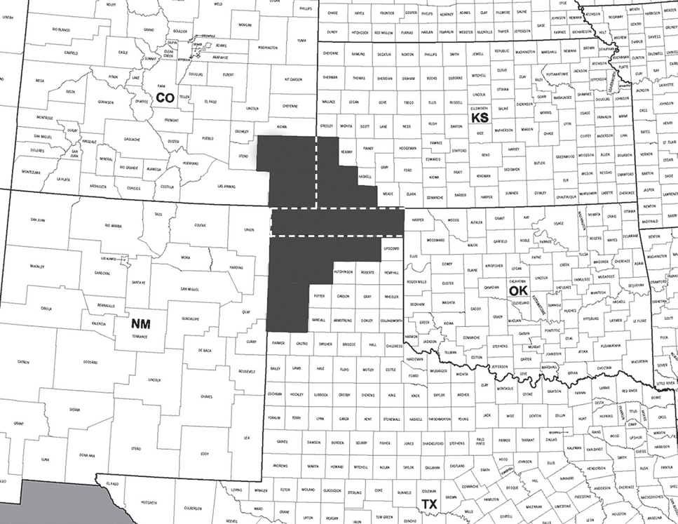
Figure 1 Dust Bowl Counties
We follow the SCS by defining the Dust Bowl counties as these 20 counties in Colorado, Kansas, Oklahoma, and Texas.Footnote 7 The 4,210 observations in our Dust Bowl dataset constitute an 11 percent sample of heads most severely affected by the Dust Bowl. In comparing the population of these 20 counties between the 1930 and 1940 censuses, this region experienced a sharp 19.2 percent drop, from 120,859 to 97,606. This compares with population growth of 4.8 percent experienced by the same four states as a whole, during the same decade.
Migration Rates
Inter-County and Inter-State Migration
We first address how geographic mobility differed in the Dust Bowl region from elsewhere. Did residents of the most drought-affected and wind-eroded counties move at a higher rate than residents from elsewhere? To answer this question we compute the fraction of residents in 1930 who were no longer living in the same place when surveyed in the 1940 census. In what follows, “place” will refer alternately to the geographic region of county and state.
Table 2 summarizes these results. The first row presents the fraction of heads who migrated across counties between 1930 and 1940. The first column presents results for those living in a Dust Bowl county in 1930, the second column for those originating from all other counties in the United States (what we will refer to as the “U.S. sample,” hereafter) in 1930.Footnote 8 As is obvious, the rate of inter-county migration was very high in the Dust Bowl: more than half (51.6 percent) of all heads originating from such counties were residing in a different county in 1940. This was approximately 1.8 times that of the inter-county migration rate (28.9 percent) observed in the U.S. sample.Footnote 9
Table 2 Geographic Mobility Rates

Notes: Mobility rates represent migration rates from sample of male household heads residing in Dust Bowl counties in 1930 and 1920 (columns 1 and 4) and all other U.S. counties in 1930 and (columns 2, 3, and 5). Standard errors of sample proportions shown in parentheses.
Source: See text for details.
This stark difference in mobility could simply reflect differences in rural versus urban composition between the Dust Bowl region and elsewhere. While the Dust Bowl counties were largely rural, the U.S. population as a whole was split much more evenly between rural and urban locales.Footnote 10 The third column of Table 2 presents statistics for U.S. heads residing in rural (non-Dust Bowl) areas in 1930. As indicated in the first row, only 28.3 percent of such individuals moved across county lines during the decade, a rate very similar to those from the United States as a whole. Hence, the high rates of migration observed in the Dust Bowl were not shared by other rural populations.
More generally, the difference in mobility does not reflect a difference in the composition of individual-level characteristics between the Dust Bowl and elsewhere. This is evident in Table 1: demographic composition is largely similar across samples.Footnote 11 As a result, little of the difference in the rate of inter-county migration between the Dust Bowl and other parts of the United States can be attributed to differences in demographic composition across regions. Instead, differences in mobility reflect differences in the propensity to migrate for particular demographic groups. Online Appendix F formalizes this via Oaxaca-Blinder analysis, decomposing the differences in migration rates into explained and unexplained effects (Oaxaca Reference Oaxaca1973; Blinder Reference Blinder1973).
While drought and erosion were experienced throughout the Great Plains, conditions were not as uniform in their severity when compared to our Dust Bowl region. Migration rates were also not as high. Of the 4,335 observations in our U.S. sample, 540 resided in the Plains states in 1930 (Montana, Wyoming, Colorado, New Mexico, North Dakota, South Dakota, Nebraska, Kansas, Oklahoma, and Texas), but outside of the 20 Dust Bowl counties. Though not presented in Table 2, the inter-county migration rate between 1930 and 1940 for this subsample was 36.8 percent, a value closer to those observed outside of the Dust Bowl than within it.
The fourth column presents statistics for heads in the same 20 counties as in column one, but residing there in 1920. Though wheat prices had fallen from their peak during WWI, the 1920s were a period of expansion in the Southern Plains, as good growing conditions and increasing mechanization led to higher yields and agricultural output (Worster Reference Worster1979). This led to a population boom during the 1920s: according to the decennial censuses, in the counties most severely affected by the Dust Bowl a decade later the population had grown from 97,473 in 1920 to 120,859 in 1930 (U.S. Bureau of the Census 1900–1990). During this period of extraordinary population growth, the region exhibited an inter-county migration rate of 47.2 percent. This is remarkably similar to the rate of the 1930s. Hence, the high rate of mobility in the Dust Bowl relative to the rest of the United States was characteristic of the region, and not necessarily symptomatic of the hardships experienced during the Dust Bowl.
The fifth column presents statistics for the U.S. sample during the 1920–1930 decade. This allows for a “difference-in-difference” perspective on mobility. As is clear, inter-county migration in the United States fell during the decade of the Great Depression, on the order of 8 percentage points relative to the 1920s. Hence, what is unusual about the Dust Bowl is not the high rate of migration per se, but the fact that it increased slightly relative to the 1920s.
The second row of Table 2 presents the inter-state migration rate. Given data limitations of previous studies, this coarser measure of geographic mobility has been the subject of analysis in other work (Rosenbloom and Sundstrom Reference Rosenbloom and Sundstrom2004). As with inter-county migration, inter-state migration was much higher in the Dust Bowl. Approximately one-third of heads originating from a Dust Bowl county in 1930 had moved to a different state by 1940, a rate nearly 2.5 times that of heads in all other counties, rural or otherwise. In the 1920s, the inter-state migration rate in this region was, again, similarly high (31.2 percent). At the national level, migration fell during the 1930s relative to the previous decade. Again, this indicates that Dust Bowl migration was atypical in its rate of change, not in its level.
Where Did They Move?
Given the high rates of mobility, where did Dust Bowl migrants go? Did their migration patterns differ from those originating elsewhere, or from those originating from the same place a decade earlier? What was the role of out-migration in the depopulation of the Dust Bowl? Table 3 presents the fraction of inter-county migrants residing in specific locations in the terminal year census. The first row of column 1 indicates, perhaps surprisingly, that of the Dust Bowlers who made an inter-county move, 11.6 percent simply moved to one of the other Dust Bowl counties. The first row of the second column presents the same statistic for migrants from the region, ten years prior. Of all inter-county migrants in the 1920s, 18.6 percent moved to one of the other 19 counties. Hence, compared to the 1930s, a greater fraction of the mobility during the 1920s represented “churning” or turnover within the region. By contrast, more of the mobility represented “exodus” or out-migration from the region during the Dust Bowl.
Table 3 Migration Destinations Probabilities

Source: See text for details.
Nonetheless, the depopulation of the Dust Bowl was not due to an extraordinary exodus relative to historical norms. Between 1930 and 1940, given the inter-county migration rate of 51.6 percent, the out-migration rate from the Dust Bowl was 0.516×(1−0.116) = 45.6 percent. Between 1920 and 1930, the out-migration rate was only somewhat lower at 38.4 percent. As such, the Dust Bowl depopulation was due largely to a sharp fall in the flow of in-migrants. Given these out-migration rates and the Census Bureau’s data on fertility and mortality, we are able to provide estimates on in-migration to the region; see Online Appendix C for details. Expressed relative to the source year population of the 20 counties in question, the in-migration rate between 1920 and 1930 was approximately 47.3 percent; during the 1930s, the in-migration rate plummeted to about 15.5 percent.
A simple counterfactual exercise puts these numbers into perspective. The population of the Dust Bowl fell from 120,859 in 1930 to 97,606 in 1940. Holding constant the number of births, deaths, and in-migrants at their observed 1930s values, if the out-migration rate from the Dust Bowl had equaled its 1920s value, the population in 1940 would have been 106,308. Therefore, lowering out-migration to its rate in the previous decade would not have prevented a population decline. By contrast, holding the number of births, deaths, and out-migrants constant at 1930s values, had the in-migration rate equaled its 1920s value, the population in 1940 would have increased to 136,079.
Hence, the depopulation of the Dust Bowl was due primarily to the fall in in-migration. Prior to this study, representative data allowing for the decomposition of the role of in- and out-migration to the 1930s depopulation did not exist. Malin had conjectured that population decline experienced in Kansas between 1930 and 1935 was due to a fall in in-migration. Malin (Reference Malin1935) and Malin (Reference Malin1961) find a decrease in the turnover of farm operators in 1930–1935, relative to 1925–1930, in a sample of 48 Kansas townships, as documented in the state census farm schedule records. Cunfer (EH.net), largely drawing on Malin, claims that high rates of out-migration were not unusual in the region. Malin’s conjecture was based on an extrapolation of the patterns in farm operator turnover as representative of population out-migration. Our findings confirm this conjecture for a comprehensive, random-sample of individuals for the Dust Bowl region, for the entire 1930s decade.
Returning to Table 3, taking the first two rows together, 62.9 percent of the Dust Bowl migrants were still residing in one of the Dust Bowl states (of Colorado, Kansas, Oklahoma, Texas) in 1940. Only 37.1 percent of all migrants left those four states. This indicates that Dust Bowl movers did not move “too far.”Footnote 12 During the 1920s, 30.7 percent of inter-county migrants left the four Dust Bowl states. Hence, the probability of leaving the Southern Plains was only slightly higher during Dust Bowl.
To better quantify the proximity of Dust Bowl relocations, we calculate the physical distance of moves for inter-county migrants. We measure this “as the crow flies,” from the centroids of the county of residence in the source year and terminal year censuses. Figure 2 presents the histogram of migration distances for both decades. The black (solid) bars are for the 1930s, the grey (hatched) bars for the 1920s.

Figure 2 Histogram of Migration Distances
Inter-county migrants from the Dust Bowl tended to make slightly longer moves, relative to their regional counterparts from the previous decade. The median migration distance in the 1930s was 300 miles; in the 1920s, the median distance was 205 miles. By way of comparison, this difference is less than the 166-mile width (measured east-to-west) of the Oklahoma and Texas panhandles.
The tendency for longer moves in the 1930–1940 decade is evident essentially throughout the distance distribution. The interquartile range during the Dust Bowl was 130–600 miles, compared to 70–500 miles during the 1920s. At the 90th percentile, the distances converge at approximately 1,000 miles; this is the distance required, for example, to move from the centroid of the Dust Bowl region to Kern County, California, at the southern tip of the agriculturally intensive San Joaquin Valley.
To visualize this, Figure 3 displays a heat map of the terminal year county of residence for inter-county migrants from the region. The top panel displays the 1940 location data for the Dust Bowl migrants, while the bottom panel displays the 1930 location data for the 1920s migrants. Darker shades indicate locations of greater migration incidence, lighter shades the opposite.
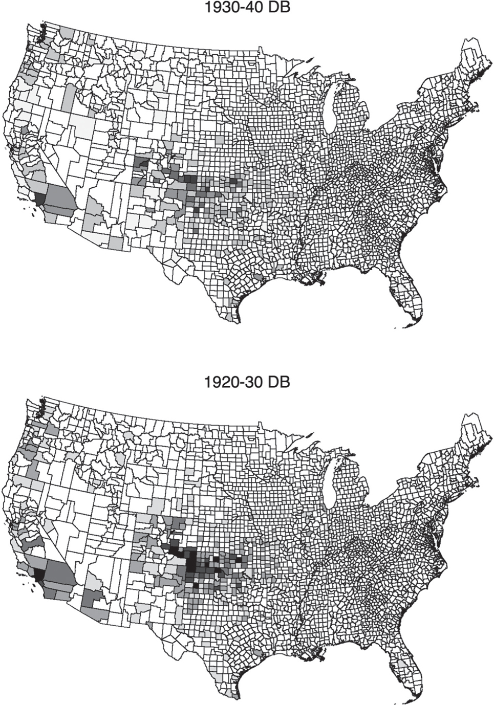
Figure 3 Heat Map of Migration Destinations
Migrants in the 1920s tended to move to counties within, or close to, the Dust Bowl region: destination locations are concentrated in southeastern Colorado, southern Kansas, and the panhandles of Oklahoma and Texas. Migration destinations were more dispersed in the 1930s, with noticeably lower concentration within the Dust Bowl counties. Instead, migrants moved to western portions of Colorado, central Oklahoma, south of the Texas panhandle, as well as New Mexico and Missouri with greater frequency.Footnote 13 This corroborates the results presented in Table 3 and Figure 2: while the median migrant moved approximately 100 miles further in the 1930s compared to the 1920s, this additional distance did not translate into moves outside of the Dust Bowl states or their adjacent states with much greater frequency.
A widely held perception—made popular, in part, by Steinbeck’s Joad Family—is that Dust Bowl migrants moved to California en masse. While a powerful image, it is far from accurate. The results presented in Figures 2 and 3 indicate that relatively few made such a drastic move.
Despite intense interest, data on Dust Bowl–California migration was severely lacking prior to this study (Worster Reference Worster1979). Based on quarantine inspection reports from the California Department of Agriculture during 1935–1936, vehicles entering the state with “persons in need of manual employment” were largely from southern drought states (Taylor and Vasey Reference Taylor and Vasey1936; Rowell Reference Rowell1936). Using data on public school enrolment, Charles S. Hoffman (Reference Hoffman1938) and Seymour J. Janow (Reference Janow1940) found that migrants to Oregon and California were disproportionately from the Plains states. Of course, such data do not shed light on the probability migrants chose California over other destinations from the perspective of the source location.Footnote 14 As such, the view that Dust Bowl migrants were overwhelming destined for California is based on incomplete data, at best.
Table 4 provides greater context. As indicated in the first row, less than 10 percent of inter-county migrants moved to California. Dust Bowl migrants were in fact more likely to move to another Dust Bowl county. Moreover, the rate at which they moved to California (9.82 percent) was largely similar to that of migrants from elsewhere in the country (7.54 percent) during the 1930s (the latter statistic excludes those living in California in 1930). The second row illustrates this from a slightly different perspective: it indicates the fraction of movers who went to California, conditional on an inter-state move. This probability was virtually identical for those from the Dust Bowl and everywhere else. This is true despite the fact that the vast majority of non-Dust Bowl migrants originated from places substantially further to the east and north.
Table 4 Moving to California

Notes: Probabilities represent fraction of inter-county and inter-state migrants residing in California in terminal year.
Source: See text for details.
Comparing the first and fourth columns of Table 4, migration to California from the Dust Bowl was also similar to that experienced from the region in the 1920s. Given either an inter-county or inter-state move, the probability of moving to California actually fell relative to the previous decade.Footnote 15 This contrasts with the findings for the rest of the United States; columns 2 and 5 indicate that, at the national level, migration to California rose from the 1920s to the 1930s.
In results not reported in Table 4, we find that, conditional on an inter-county move, the fraction of Dust Bowl migrants who moved to any of the west-coast states of California, Oregon, and Washington was 14.9 percent; in the 1920s, the fraction of migrants moving to the west coast was 13.9 percent. Finally, we compute the longitudinal direction of moves using the centroids of the county of residence in the source and terminal year censuses. In the 1930s, 45.9 percent of migrants from the Dust Bowl moved in a westerly direction relative to their 1930 location. This compares with 45.6 percent in the previous decade. As such, our data indicate that the “westward push” from the Dust Bowl was unexceptional during the 1930s.
When Did They Move?
The 1940 census was the first to ask respondents of their location of residence five years prior, in 1935. Given that this information was self-reported, it is less accurate relative to the respondents’ information for 1930 or 1940 along two key dimensions: (1) whether the “five years ago” information pertained precisely to the year 1935, and (2) whether the name and spelling of the county of residence were reported and recorded correctly. Nonetheless, this information allows us to determine how geographic mobility in the Dust Bowl was approximately distributed across the early and latter parts of the decade. This is of interest, given that while the economic and environmental effects of the Dust Bowl were felt throughout the 1930s, many of the agriculture-related New Deal programs were initiated in the early-to-mid portions of the decade.
Table 5 indicates the location patterns of Dust Bowl migrants between 1930 and 1940, for those whose location of residence in 1935 could be accurately discerned. In the table, we denote the county of origin in 1930 by the letter A, and the destination county in 1940 by the letter B. The first row indicates that approximately one quarter of Dust Bowl migrants were still living in their county of origin in 1935. By contrast, 52.8 percent had already moved to their destination county by 1935. Rows three and four indicate the fraction of migrants who were in a third location, C, in 1935 (that was neither their 1930 nor 1940 residence). A non-negligible fraction (21.8 percent) made an “indirect” move between points A and B during the decade. Hence, the vast majority of Dust Bowl migrants had already moved by mid-decade.
Table 5 Migration Patterns, 1930 → 1935 → 1940

Notes: Migration patterns represent fraction of inter-county migrants, originating from the Dust Bowl, by location of residence in 1935.
Source: See text for details.
This fact is particularly interesting given that prior to this study, data on migration spanning the entire decade were unavailable. Indeed, the literature’s conclusions on Dust Bowl migration are based largely on the 1935 and 1940 location data obtained from the 1940 census (Worster Reference Worster1979). The results in Table 5 indicate that 52.8 + 18.1 = 70.9 percent of the observations on inter-county migration that we identify through census linkage would have been missed by simply using the 1935 location of residence information from the 1940 census.Footnote 16
Who Moved?
As documented in the previous section, migration rates were much higher among Dust Bowlers compared to other Americans. In this section, we investigate the correlates of mobility using data on individual-level and county-level characteristics available from the census and other sources. We begin by analyzing how inter-county migration probabilities covaried with individual characteristics. Let πi be a dummy variable that takes on the value of one if individual i moves across counties between 1930 and 1940, and a value of zero otherwise. We consider a simple linear probability model for migration: ${\pi _i} = {X_i}\beta + { \in _i},$
where, Xi denotes characteristics of individual i in 1930.
Included in Xi are standard demographic controls for age, marital status, and years of schooling.Footnote 17 The 1930 census also allows us to determine whether an individual is a “head of family” or not (e.g., boarder, lodger); owns or rents his home; is living in his birth state or not. In terms of parental information, we can determine the number of children, and the age of each child belonging to the head. We include a dummy variable for whether a child under the age of five years is present in the household; based on our analysis of various ways to control for parenthood, this contained the most explanatory power.
We also include the individual’s 1930 occupational information. Not surprisingly, the distribution of occupations in the Dust Bowl sample differs quite dramatically from that of the U.S. sample, and in particular, from the distribution observed in urban areas. For purposes of comparison, we choose to summarize the occupational information into four broad, mutually exclusive categories: farmers who are, by definition, self-employed; farm laborers who are, by definition, wage workers; nonfarm self-employed; and non-farm wage workers.
In 1930, respondents reported whether they owned a “radio set,” the first time the census of population asked about a consumer good in the main questionnaire. Households with radios may have been more informed than those without, particularly with respect to economic conditions beyond the local area, pertinent to migration choice. We include this information as both a proxy for wealth and access to news and information.
The first column of Table 6 presents results for the sample of heads residing in Dust Bowl counties in 1930. The reference (or excluded) group in the regression are: 46–60 year old, married, family heads with at least one child under the age of five, farmers, renters, non-radio owners, not living in their state of birth, with fewer than eight years of (primary) schooling.
Table 6 Correlates of Inter-County Migration

Notes: Coefficient estimates from the linear probability model, equation (1). Regression is sample weighted; robust standard errors in parentheses.
Source: See text for details on variables.
The estimated coefficients are largely of the expected sign and relative magnitudes. For instance, there is a strong negative relationship between age and mobility, with 16–25 year olds 14.7 percentage points more likely to move counties relative to 46–60 year olds (significant at the 1 percent level).Footnote 18 We refer to family or non-family headship, marital status, and having young children collectively as “family structure” covariates, hereafter. Not surprisingly, being a family head has a strong negative association with migration probability (significant at the 1 percent level). But surprisingly, the conditional correlations of marital and parental status with migration are statistically indistinguishable from zero. Living in one’s birth state likely means having greater family or economic ties to the place of residence, and is plausibly viewed as measuring a cost of migration. Interestingly, there is no relationship of this variable to migration for those in the Dust Bowl.
Homeownership and radio set ownership—both proxies of wealth—are strongly and significantly associated with lower mobility. Owning a radio could also measure access to information about economic conditions (Ziebarth Reference Ziebarth2013). Under this interpretation, the negative association could indicate that those more informed about the wide-reach of the Dust Bowl and Great Depression were less likely to believe migration would improve well-being.
Most importantly, relative to all other occupations, farmers (the reference group) have a lower probability of moving. The occupational differences are large and statistically significant at the 1 percent level. Hence, of all occupations, farmers were the least likely to move from the Dust Bowl. This may seem unsurprising if farmers are those who possess the most location-specific human and physical capital. However, to the extent that this is true, this is not borne out for farmers elsewhere in the country. In the United States as a whole, it appears that farmers were approximately equally likely to move as were men in other occupational categories, as evidenced by the small and statistically insignificant coefficient estimates shown in columns 2 and 3 (discussed later). The relative immobility of farmers in the Dust Bowl region does not reflect a national pattern. This finding is surprising given the popular notion of the migrant Dust Bowl farmer expelled from the land, as portrayed in literature, art, and music.
Finally, it is worth noting that education is not clearly or strongly related to migration propensity in any of the three samples represented in Table 6. This is relevant for considering migrant selectivity and the economic effect of migration, as we do in the following section. At least from this measure, it looks as if education does not play a role in any migration selection on skill or human capital.
The second column of Table 6 presents results for individuals living elsewhere in the United States. Though some results are similar to those in column 1, there are important differences. First, all occupation groups have statistically indistinguishable probabilities of migration; farmers outside of the Dust Bowl were no more or less likely to move than others.
The estimated coefficients on family structure variables are all associated with significantly higher migration probabilities in the U.S. sample.Footnote 19 Being married, having a family, and having young children represent mobility costs. Likewise, living in one’s birth state has a strong negative association with migration. These effects are substantially weaker in the Dust Bowl. In conjunction with the findings provided later in Table 7, this is indicative of a greater degree of “turnover migration” of individuals in the Southern Great Plains region.
Table 7 Correlates of Dust Bowl Region Migration: 1920s vs 1930s

Notes: Coefficient estimates from the linear probability model, equation (1). Regression is sample weighted; robust standard errors in parentheses.
Source: See text for details on variables.
In the third column of Table 6, we consider the sample of heads in rural counties outside of the Dust Bowl. As discussed in the previous section, the high rates of migration observed in the Dust Bowl were not shared by other rural areas. Here, the objective is to determine whether the differences in the covariation of individual characteristics and migration across samples are also evident when comparing the Dust Bowl to other rural areas. Indeed, we find that the estimated differences remain. The regression results for the rural U.S. sample are largely the same as the U.S. sample that includes both urban and rural heads. Hence, the differences in the correlates of migration observed in the Dust Bowl relative to outside the Dust Bowl are not shared by other rural populations.
We have conducted a series of robustness checks which, for the sake of brevity, we present in Online Appendices D and E. First, we repeat the analysis on inter-county migration replacing the linear probability model, equation (1), with a probit model. Not surprisingly, the results are essentially identical to those generated from the linear specification. We also extend our analysis by augmenting the individual-level covariates with a number of variables at the county-level, as considered in Price V. Fishback, William C. Horrace, and Shawn Kantor (Reference Fishback, Horrace and Kantor2006). This allows for comparison of our results on gross migration (at the individual level) with their results on net migration (at the county level). In addition, we repeat the analysis of Table 6 considering inter-state migration. Overall, the results for inter-state migration are similar to those for inter-county migration; the salient differences between Dust Bowl and non-Dust Bowl counties remain intact.
Comparing the 1920s and 1930s
In the previous section, we documented how migration in the Dust Bowl region was similar when comparing the 1930s and 1920s decades. In this sense, the high mobility rates in the Dust Bowl relative to the rest of the United States were characteristic of the region. Here, we examine whether observables’ influence on migration choices was similar for inhabitants of the region across decades, or whether the estimated effects from Table 6 were specific to the Dust Bowl episode.
Table 7 presents the results from the estimation of equation (1) on the Dust Bowl samples of the 1920s and 1930s. For the 1920s regression, πi indicates whether individual i moved between 1920 and 1930, and Xi denotes individual-level characteristics in 1920. Since information on education is not available for the 1920s sample, we omit these variables from the regression specification.
Comparing columns 1 and 2 reveals a large degree of similarity across decades in the estimated coefficients on inter-county migration.Footnote 20 But a couple of differences are worth noting. First, living in one’s birth state has no effect on migration probability in the 1930s. By contrast, birth state has a strong negative relationship in the 1920s, just as it does for the rest of the United States in the 1930s. That individuals viewed the cost of leaving one’s birth state as negligible, relative to the benefit of moving, is unique to the Dust Bowl experience. This is, perhaps, indicative of the migratory “push” generated by the Dust Bowl’s poor economic conditions. A second, subtle difference is that the non-farm self-employed were more likely to move county or leave the region than were farmers in the 1930s, but in the 1920s that difference was very small and statistically insignificant. Wage earners were the most likely to move in both decades but the difference between farmers and the rest was sharpest in the 1930s, whereas the 1920s was marked by a difference between wage earners and self-employed, both on and off the farm.
Finally, as previously documented, a greater fraction of inter-county migration represented exodus from the region during the Dust Bowl compared to the 1920s. Table 7, columns 3 and 4, present estimates of equation (1) where the dependent variable is an indicator for leaving the set of 20 Dust Bowl counties. The results are largely unchanged relative to those for inter-county migration presented in columns 1 and 2.
As discussed, the majority of Dust Bowl migrants moved prior to 1935. We also investigate whether early-decade and late-decade migrants differ systematically in terms of observable characteristics. Briefly, we find such evidence; detailed results are discussed in Online Appendix E. Finally, we analyze the correlates of moving to California during the 1930s, and how these differed for Dust Bowl migrants compared to others. Perhaps most interestingly, those working in agriculture were no more likely to move to California than others. This contrasts with the popular notion that those who went west were displaced farmers and farm laborers seeking agricultural work in California’s produce fields and orchards. Again, we refer the reader to the Online Appendix for details.
The Migrants’ Economic Gains
The linked dataset is well suited to assessing the impact of migration on individuals’ economic outcomes during the 1930s decade. Because we observe location in both 1930 and 1940, and occupation in 1940, it is straightforward to estimate the effect of the decision to leave or remain in the Dust Bowl region on one’s “occupational earnings,” that is, the average annual earnings for each occupation (fully defined later). Furthermore, unlike many empirical migration studies, we observe an individual’s initial occupation in 1930, before the migration decision is made. We use this information to control for individual-level characteristics that could influence the migration decision.
Migrant Selection
As we discuss in the previous section, migrants differ from non-migrants along several observable dimensions. Following David McKenzie, John Gibson, and Steven Stillman (Reference McKenzie, Gibson and Stillman2010) and William Collins and Marianne Wanamaker (Reference Collins and Wanamaker2014), we assess migrant selectivity by estimating the relationship between occupational earnings in 1930 and the subsequent migration decision: ${\pi _i} = \theta {y_{i,1930}} + {X_i}\beta + { \in _i}.$
Throughout this section, πi takes on the value of one if the individual leaves the Dust Bowl region; πi = 0 for Dust Bowl persisters—those who did not move or, conditional on migration, remained in one of the 20 Dust Bowl counties. This differs from previously, where πi was an indicator of inter-county migration. In the context of the outcome effect of migration, leaving the Dust Bowl is the more natural measure. Not surprisingly, since approximately 90 percent of inter-county migrants left the Dust Bowl region (see Table 3), the results are not sensitive to this choice.
Unfortunately, the 1930 census contains no information on income or earnings, and the 1940 census includes income only for wage and salary earners (earnings for employers and the self-employed, including farmers, are not recorded). Both censuses do contain information on occupation. Therefore, y i,1930 is log 1930 earnings imputed on the basis of occupation. This is the “occscore” variable from IPUMS, generated by crosswalking the 1930 occupations to 1950 occupation codes, then assigning observations the median income level for each occupation in 1950 (see also Abramitzky, Boustan, and Eriksson Reference Abramitzky, Boustan and Eriksson2012; Collins and Wanamaker Reference Collins and Wanamaker2014). This allows for the measure of median earnings differences across occupations, but not differences within occupation. Throughout, we refer to this variable as “occupational earnings.”
The individual-level controls, Xi , includes age group, education, the “family structure” variables, homeownership, living in birth state, and a state-level dummy variable. When Xi is omitted from equation (2), θ is a simple measure of migrant selectivity; with Xi included, θ measures “selection on unobservables.” In either case, θ > 0 indicates that migrants were positively selected, θ < 0 they were negatively selected.
For brevity, we summarize here and make details of our results available upon request. Estimating equation (2), there is evidence of mild positive selection on unobservables (θ = 0.0482, s.e. = 0.0182); this is balanced by mild negative selection on certain observables (such as family headship and home ownership). As a result, estimating equation (2) without controlling for Xi , we find no appreciable evidence of selection among the Dust Bowl migrants (θ = 0.0198, s.e. = 0.0178).
It is instructive to put this in context with other migration episodes. One straightforward comparison is with out-migration from this same region in the 1920s (a period when gross migration rates were high, as previously). Estimating equation (2) on the 1920s sample without controlling for Xi , we find stronger evidence of positive selection: migrants were 5.7 log points greater than non-migrants, and this difference is statistically significant at the 5 percent level. Controlling for Xi , we also find positive selection on unobservables. However, it should be noted that data on educational attainment, an important determinant of earnings, is not available for the 1920s sample. Migrant selectivity during the Dust Bowl was also small relative to two other important U.S. migration episodes. African-American participants in the Great Migration of the early twentieth century had pre-migration earnings ten to 15 log points higher than non-migrants (see Collins and Wanamaker Reference Collins and Wanamaker2014). And while differing methodologies prevent direct comparison, Abramitzky, Boustan, and Erkisson (Reference Abramitzky, Boustan and Eriksson2012) find strong evidence of negative selection among urban Norwegian migrants to the United States during the age of mass migration in the nineteenth and early twentieth centuries.
What Happened to the Migrants?
To study the association between the migration decision and subsequent economic outcome for the individual, we estimate a simple model of change in individual occupational earnings via OLS: ${y_{i,1940}} - {y_{i,1930}} = \tau {\pi _i} + {X_i}\beta + {v_i}.$
Again, yi,t is log occupational earnings in t ∈ {1930,1940}, πi equals 1 if the individual leaves the Dust Bowl and 0 otherwise, and Xi are covariates that we discuss later.
Migration status is not exogenous; migrants and persisters differed. However, as our analysis of equation (2) shows, there does not appear to be strong migrant selectivity. Furthermore, the fact that we observe occupation at both points in time allows us to estimate the impact of migration on change in occupational earnings between 1930 and 1940, rather than on the 1940 level. Importantly, this difference-in-difference approach accounts for all time invariant, individual-level characteristics that might otherwise introduce selection bias into our estimate of τ.
The top panel of Table 8 displays estimation results of equation (3), both with and without individual-level controls. We account for the possibility of differential occupational earnings growth by age and education by including these successively as Xi , in columns 2–4. We also include a specification with county-level fixed effects. Estimating equation (3) on all individuals in our Dust Bowl sample indicates a statistically significant, but economically small increase in occupational earnings for migrants; the results are quite stable across specifications. According to our richest specification in column (4), those who left the Dust Bowl experienced occupational changes that translated to a 3.3 percent increase in earnings on average.
Table 8 Occupational Earnings and Migration

Notes: Coefficient estimates from the occupational earnings growth regression, equation (3).
Source: See text for details on variables.
This, however, masks important differences between the roughly half of our sample who were farmers in 1930 and the half who were not. This is shown in the bottom panel of Table 8. Conditional on being a farmer in 1930, migrants had 1940 occupational earnings between nine and 11 log points greater than those who stayed in the region; this is significant at the 1 percent level.
In assessing economic outcomes, farmers are notoriously difficult to characterize using historical U.S. census data, which does not differentiate between more and less prosperous farmers. There is no straightforward solution to this problem, as the census records only occupation. One might be concerned that the results of Table 8 are driven by the relatively low occupational earnings assigned to farmers: $1,400 versus the median $2,000. We assess the sensitivity of our results to the position of the farmers in the earnings distribution in two ways. First, we re-estimate equation (3) omitting all cases where farmers transition to unskilled laborers, an occupation with a slightly higher average annual earnings that, nevertheless, would likely have been an occupational downgrade. The results are essentially unchanged. Second, we re-estimate equation (3) using the Duncan Socioeconomic Index (SEI) measure in place of occupational earnings (Duncan Reference Duncan1961), where farmers are the median SEI occupation. The results are very similar to those obtained from occupational earnings: farmers who migrated realized a large, statistically significant gain in SEI, whereas in the whole sample we observe a smaller positive effect that is statistically significant in some, but not all specifications.
To shed light on these results, Table 9 displays transition matrices across broad occupational groups for migrants and persisters. Occupations are grouped based on their earnings. Farmers in 1930 who left the Dust Bowl were more likely than persisters to experience downward occupational moves, becoming laborers in 1940 (21.6 versus 8.6 percent). However, this tendency for greater downward mobility was more than offset by their greater likelihood of experiencing upward moves toward semi-skilled or high-skilled occupations (39.0 percent for migrants versus 19.0 percent for persisters). The negative migration effect for non-farmers is driven primarily by the greater tendency of high-skilled migrants to transition into semi-skilled occupations relative to persisters (who were more likely to remain in a high-skill occupation). This more than offsets the effect of greater tendency among migrant laborers to move up the occupational ladder, relative to their counterparts who stayed.
Table 9 Occupational Transition Matrices: Migrants vs. Persisters

Notes: Values in rows indicate the probability that individuals from one occupation group in 1930 (arranged by column) transits to each occupation group in 1940. High-skilled = manager, official, proprietor, etc.; semi-skilled = carpenter, mechanic, salesman, etc.; laborer = general laborer and farm laborer. Detailed information on occupation groups available from authors upon request.
Source: See text for details.
Clearly, contrary to long-standing popular perception, the typical Dust Bowl migrant was not destined for economic hardship and loss. On average, migrant farmers—far from ending up as marginalized, poorly paid agricultural laborers—enjoyed better occupational outcomes than did those who persisted. Also, the most typical downward occupational move associated with migration was a greater tendency for high-skilled migrants to transition to semi-skilled occupations, a move that, while associated with a loss in earnings on average, was not associated with falling into poverty. Two caveats apply. First, we only observe individuals once in 1930, then once again ten years later. In light of this, we cannot, for example, rule out the possibility that migrants experienced significant hardship between the time of migration and 1940, only that negative outcomes that persisted until 1940 were not prevalent. Nor can we rule out the possibility that individuals experienced a negative occupational shock before moving, making the economic effect of migration appear more negative than it might have been. Second, because we observe only occupation and impute earnings, it is possible that some individuals who made upward occupational moves earned less in 1940 than in 1930 (and, of course, vice versa). The potential error associated with using imputed rather than observed earnings could be more acute for farmers, for whom there was large variance in earnings nationally. However, the likelihood that we are significantly understating earnings losses of migrants who transitioned out of farming is mitigated in this specific case by the fact that high-earning, large landholding farms were uncommon in the Dust Bowl region in the 1930s.
Conclusion
The Dust Bowl of the 1930s was one of the most severe environmental economic shocks in U.S. history, and it is associated with one of the most prominent internal migration episodes. We know from previous research that the Dust Bowl had a long-lasting impact on the region itself. Land use adjustment was slow and agricultural land value was depressed for decades (Hornbeck Reference Hornbeck2012). But tracking the individuals most affected by the crisis reveals that they were able to mitigate the negative impact of the Dust Bowl on their own economic condition via migration. Those who chose to leave bettered their economic situation relative to those who stayed even by the end of the decade, at least in terms of occupational transitions. Contrary to durable popular perceptions, they did not rely on migration to California to an exceptional degree. Dust Bowl migrants moved to California at approximately the same rate as did internal migrants from elsewhere in the United States. Instead, relatively local moves were the norm. In our data, migrants tended to relocate from counties hardest hit to less-impacted counties within the Southern Great Plains region, and short-distance moves were most common.
Our empirical framework cannot conclusively demonstrate what motivated the migrants. However, our findings are broadly consistent with the notion that these were indeed “distress migrants,” pushed from the region by the large, exogenous climate shock. Family-related factors, such as being married and having young children, which typically impeded migration were significantly less efficacious in the Dust Bowl region in the 1930s. Furthermore, there is no evidence of overall migrant selectivity in the 1930s, in contrast to migration from the same area in the 1920s and from other migration episodes in U.S. history. Both of these results indicate that these were likely to be distress moves of necessity, rather than the sort of calculated economic decisions often associated with migration.
Migration rates in the Dust Bowl region were exceptionally high in the 1930s not with respect to the 1920s, but with respect to the rest of the country. While it appears that in the country as a whole migration declined in the 1930s relative to the 1920s, in the Dust Bowl region it rose slightly. Hornbeck (Reference Hornbeck2012) shows that the local economies of the most heavily affected counties adjusted in the long run primarily through large relative population declines. We find that this decline was caused not by an exceptional exodus of migrants, but by a dramatic decline in migration into the region. This was an area of significant population turnover. Given the marginal nature of the land on the western agricultural frontier, this is perhaps not surprising.
Considering the important role of out-migration in individuals’ adjustment to the Dust Bowl, it seems clear that mitigation of this climate shock was facilitated by a regime of high overall internal mobility. The high turnover migration pattern of the 1920s, marked by extensive in- and out-migration, was replaced by a pattern in the 1930s of slightly elevated out-migration and dramatically reduced in-migration. To the extent that this adjustment mechanism—sustained outflow, decreased inflow—is common, it suggests that places with greater mobility may be more robust to regional economic shocks, environmental and otherwise. Individuals in such high mobility regimes would be less affected by such shocks in the long run, even if the impact on specific locations is long lived. This has obvious present-day implications for places where climate change raises the prospect of environmental shocks similar in their catastrophic localized impact to the U.S. Dust Bowl of the 1930s. In addition, to the extent that internal migration is declining in the United States overall (Molloy, Smith, and Wozniak Reference Molloy, Smith and Wozniak2017) and the country transitions to a lower-mobility regime, it could lead to diminished economic resilience to localized shocks if the populace is less able or willing to respond via migration than was the case in the past.


