


1. Introduction
The promotion of gender equality, together with the economic and social empowerment of girls and women, has been reassessed to form a global goal of the 2030 agenda for achieving sustainable and prosperous development. By removing the barriers that prevent women from accessing—as men do—human capital endowments, economic opportunities and human rights, gender equality may allow economies to perform better and to improve economic development. Despite improvements in gender equality and female empowerment since the achievement of the Millennium Development Goals, gender differences persist and continue to be a major challenge for both developed and developing countries. Hence, it is essential to better understand the relationship between gender equality and economic development. This paper aims at improving our understanding of gender equality and its relationship with economic development in a historical perspective.
A number of theoretical contributions have suggested the existence of a negative link between gender inequality and economic growth [e.g., Galor and Weil (Reference Galor and Weil1996), Lagerlöf (Reference Lagerlöf2003), De la Croix and Van der Donckt (Reference De la Croix and Van der Donckt2010), Prettner and Strulik (Reference Prettner and Strulik2017); among others].Footnote 1 Among them, Diebolt and Perrin (Reference Diebolt and Perrin2013, Reference Diebolt, Perrin, Diebolt, Carmichael, Dilli, Rijpma and Störmer2019) emphasized the role played by greater gender equality in the decisions made by family members (in terms of children's education, for instance) that influence in turn long-term economic and demographic changes. The empirical literature that links gender equality and economic development based on contemporaneous data is abundant [see, for instance, Goldin (Reference Goldin1990, Reference Goldin1994), Schultz (Reference Schultz1995), Dollar and Gatti (Reference Dollar and Gatti1999), Klasen (Reference Klasen2002), Knowles et al. (Reference Knowles, Lorgelly and Owen2002), Doepke and Tertilt (Reference Doepke and Tertilt2009), Klasen and Lamanna (Reference Klasen and Lamanna2009)].Footnote 2 However, few empirical studies focus on gender inequalities in earlier periods (i.e., using historical data). Among them, a few have recently measured the gender wage gap during the modern era [see Humphries and Weisdorf (Reference Humphries and Weisdorf2015), regarding England; Gary (Reference Gary2017), regarding Sweden; and De Pleijt and Van Zanden (Reference De Pleijt and van Zanden2018), with regard to a group of European countries]. These works contribute to the deeper improvement of our understanding of gender relations over the long run but can measure only one dimension of gender inequality. Yet, as shown by De la Croix and Van der Donckt (Reference De la Croix and Van der Donckt2010), the various dimensions of gender disparity have different effects on shaping the development process. Gender equality is a multidimensional concept and a comprehensive measure of gender parity must encompass a wide range of gender-based indicators if it is to capture the various dimensions of gender equality, and consequently the various channels through which gender equality may foster economic development.
Despite improvements made to measure gender equality, no equivalent tools exist at the historical level, in particular because of data limitations.Footnote 3 Consequently, our knowledge of gender (in)equality in the past remains largely limited to qualitative investigations. The paper builds an indicator measuring the size of the gender gap from a historical perspective following the methodology developed by Hausmann et al. (Reference Hausmann, Tyson and Zahidi2006)—within the project launched by the World Economic Forum in 2005. This index captures the size of the gap between men and women in four critical areas: economic participation and opportunities, educational attainment, health and survival, and political empowerment. Gender equality is considered achieved when women and men have the same rights and opportunities across all sectors of society, and when their behaviors, aspirations, and needs are equally valued and favored. Extending this line of research to a historical period, Perrin (Reference Perrin2014) proposed a first attempt to measure the size of the gender gap in the past—which is further developed in the current paper. Recently, using a similar methodology, Dilli et al. (Reference Dilli, Carmichael and Rijpma2019) calculated a gender equality index for a collection of 129 countries during the period 1950–2003. They found that countries made substantial progress in gender equality over the past 50 years but that little convergence between countries could be observed.
Based on a unique dataset built up from the Statistique Générale de la France, I created a county-level historical gender gap index measuring the extent to which women achieved equality with men across France in the 1850s.Footnote 4 Mid-nineteenth century France is a particularly interesting case to study. France was experiencing its economic takeoff while its demographic transition had already been under way for about 50 years.Footnote 5 Besides, the country presents exceptional regional diversity on various dimensions—economic, demographic, social, cultural—reflecting the different stages of development reached by the regions [see Perrin (Reference Perrin2013)]. The ambition to construct a historical gender gap index was twofold. First, this index is used to pinpoint regional variations in the distribution of opportunities and resources between genders during the modernization in France. Second, this index opens the door for new empirical insights in investigating the consequences of gender differences in the middle of nineteenth century France on the country's economic development. Using the heterogeneity of the county gender gap index, preliminary tests reveal that the French counties that came nearest to closing their gender gap display better economic performance and exhibit lower fertility rates. The analysis also shows that when comparing the effect of the sub-indices separately, the overall index—which compasses the wider variety of gender indicators—captures far more variations in economic performance than any of the sub-indices.
The remainder of the paper is structured as follows. Section 2 describes the methodology and steps followed to build the historical gender gap index. Section 3 presents the gender-based dimensions and variables necessary for the construction of the index. Section 4 presents the strengths and weaknesses of France in closing the gender gap and investigates a range of possible determinants. Section 5 provides an overview of the county-level relationship between gender-related conditions and economic performance. Section 6 summarizes and concludes.
2. Methodology: the construction of the index
This paper aims at capturing gender-based disparities in various dimensions from a historical perspective. The county-level gender gap index is constructed using a five-step process, as done by Hausmann et al. in the computation of the gender gap index 2006. This procedure is applied to all gender-related indicators integrated to build the index.
2.1 Step 1: conversion to ratios
In order to capture gender equality per se, my index measured the position reached by women relative to the position reached by men. A county was rewarded (or penalized) on the basis of the size of the gap between men and women, but not for its overall levels. This strategy enabled me to account for gender equality independently of the level of development, i.e., without economic-related a priori on the data. Indeed, people living in richer counties are likely to present greater educational attainment than people living in poorer areas. Nevertheless, such counties could exhibit wide gender inequality. Conversely, less developed counties could present low educational attainment but limited gender inequality.Footnote 6 Accounting for gaps allowed me to account for the various possible scenarios by focusing strictly on gender differences, all other factors being equal. Hence, I first converted all the data into female-to-male ratios. To give an example, a county with 30% girls and 62% of boys enrolled in primary schools was assigned a ratio of 30/62 = 0.48 on this variable. Such a ratio meant that girls had closed 48% of the gap with boys in primary school enrollment. For approximately 2 boys enrolled in primary school, then, 1 girl is enrolled.
2.2 Step 2: data rescaling and truncation at the equality benchmark
The second step of the process involved: (i) rescaling the natural female-to-male ratios to the equality benchmark; and (ii) truncating the ratios to one. The truncating procedure enabled me to assign the same score to counties that had reached parity between women and men and to those where women had out-done men. The rescaling procedure allowed me to account for natural differences between men and women. The equality benchmark was taken to be 1—meaning equal numbers of women and men—on all variables except those of health. Taking the example of the sex ratio, this gender-based indicator varied according to the age profile of the population. It may also have been affected by environmental and social factors. Grech et al. (Reference Grech, Savona-Ventura and Vassallo-Agius2002) have estimated the natural sex ratio at birth to be circa 1.06 men per 1 woman. Accordingly, the equality benchmark is set to be 0.944 to correct for the natural factors of the sex differential. Similarly, the reversed mortality ratio and the life expectancy ratio were truncated according to the equality benchmark set at 1.06.Footnote 7 I employed the reversed value of the mortality ratio to have the same sign in interpretation (i.e., the higher the value, the better the score). It integrated the positive effect of having a low mortality ratio in the health outcome. Once the indicators were rescaled to the equality benchmark (1), the ratios were truncated to 1 as the highest possible level of gender parity.
2.3 Step 3: calculation of weighted averages
The gender gap index is a composite indicator. Each gender-related dimension—based on economic, education, and health criteria (described in section 3)—constitutes the sub-indices that I used to construct the overall gender gap index. As a third step, I calculated the weighted average of the variables within each sub-index to create the sub-index scores. This computation aimed to give the same weight to each variable because some variables exhibited greater volatility than others, e.g., larger standard deviation [see Sugarman and Straus (Reference Sugarman David and Straus1988) and Harvey et al. (Reference Harvey, Blakely and Tepperman1990)]. The calculation of sub-index scores involved: (i) calculating the standard deviation for each variable; (ii) normalizing variables by equalizing their standard deviations to determine the percentage change in terms of standard deviation to a 1% change of each variable; and (iii) using these weights to calculate the weighted average of the variables.
2.4 Step 4: calculation of sub-index scores
I now turn to the way in which I calculated the weighted average score of the sub-indices. This process ensures that the same relative impact would be integrated into the sub-indices for each variable, so that a variable for which most counties had already reached equality would be penalized. For example, the wage ratio in industry has a relatively small standard deviation. The wage ratio gets greater weight in the economic opportunity sub-index, while the labor force ratio in industry has a larger standard deviation. Similarly, for any variable characterized by a higher ratio and lower variability (i.e., greater weight), a county that would deviate would be more heavily penalized.
2.5 Step 5: calculation of final scores
Finally, I calculated the scores of the indices. All the sub-indices were bounded between 0 and 1 to allow for cross-county comparisons. The value 0 corresponded to perfect imparity; 1 to perfect parity. To create the overall gender gap index, I brought together the three sub-indices by simply taking their (un-weighted) average at the county level. The final score was also bounded between 0 and 1.
3. Data
The construction of such an index was constrained by the availability of the data. I explore the size of the gender gap from gender-related variables belonging to three critical categories: (i) economic participation and opportunity; (ii) educational attainment; and (iii) health and survival.Footnote 8
3.1 Multiple dimensions of gender-based disparities
I use county-level data collected from diverse publications of the Service de la Statistique Générale de la France. The French Statistical Office publishes data since 1800. But from 1851, the Statistical Office provided data ranking population by age, gender, marital status, and other essential information used to build a measure of the gender gap. The dataset covers information about aggregated individual-level behavior for 86 French counties (départements). The major part of the dataset is constructed from general censuses, statistics of primary education, population movement, and agriculture survey conducted in the 1850s; and from industrial statistics conducted in 1861. I combined the various censuses to construct a dataset with gender-related detailed information on employment and wages in industry and agriculture, literacy rates, enrollment rates in primary schools, population, longevity, and mortality.
3.1.1 Economic criteria
Four variables were used to capture the size of the gender differences in economic opportunity and participation. The share of people employed in manufacturing and the share of people making their living from agriculture in 1851 were used to measure the difference in participation in the labor force between men and women. The average hourly wages (in francs) in industry and in agriculture were used as proxies to measure differences in remuneration.
3.1.2 Education criteria
Three variables were used to measure gender differences in education: enrollment rates, literacy rates, and public schools. Enrollment rates in public primary school measure educational attainment. Enrollment rates are calculated as the number of boys/girls attending school divided by the total number of boys/girls aged 5–15. The literacy rate is a proxy measuring the long-term ability of individuals to read and write. The third variable included in this sub-index is the number of public schools for boys/girls, used to capture the sex-differential in the infrastructure. These variables were used as a proxy to measure the differences in institutional investment between boys and girls.
3.1.3 Health criteria
Three variables were used to capture gender differences in health and survival: the number of births of boys and girls (in 1851), the mortality rate of men and women (in 1851), and the life expectancy of men and women (in 1856). The differences between the birth numbers for boys and girls may be skewed by factors such as infanticide. It reflects households' potential preference for sons (society's valuation of women) or, inversely, women's ability to protect vulnerable female children. Mortality rates were calculated as the number of men/women who died per 1,000 living men/women. Finally, the construction of a measure of life expectancy at birth involved several steps. I calculated a life table at the county level, splitting the population into 5-year age bands and the deaths into 5-year age bands (as detailed in Appendix B). These data were available for the year 1856 by combining data from the Census and from the Population Movement. Both the mortality and the life expectancy ratios captured the mortality differential potentially triggered by violence, malnutrition, or disease. Appendix A describes all the data and sources in greater detail.
3.2 Descriptive statistics of gender differences
Table 1 reports the descriptive statistics of the variable used to construct the gender gap index. The share of individuals working in the agricultural sector was high for both genders, while the share of individuals making their living from working in industries was low. In 1851, almost 74% of men and 61% of women were working in agriculture, but respectively only 6% and about 4% in industry. Moreover, the female-to-male labor force ratio was markedly higher in agriculture (0.83) than in industry (0.48). To a lesser extent, the female-to-male average wage was higher in agriculture (0.63) than in industry (0.47). However, both female and male average wages were substantially higher in industry than in agriculture; 1.08F for women in industry as against 0.89F in agriculture and 2.27F for men in agriculture as against 1.41F in agriculture.
Table 1. Summary statistics of the variables

Sources: Using data from Statistique Générale de la France.
Regarding educational variables, more than 66% of males and 50% of females in 1854 were able to read and write. In 1851, 54.4% of boys but only 36% of girls aged 6–14 were enrolled in public primary schools. Across counties, there was strong heterogeneity in education: enrollment rates went from about 19% (in Var) to 106% (in Manche) for boys and from 0.3% (in Loir-Et-Cher) to 99% (in Manche) for girls.Footnote 9 These variations could result from several factors: the diffusion of the official French language, the difference in attitudes toward education between Catholics and Protestants [see Becker and Woessmann (Reference Becker and Woessmann2009)], the wave of ideas spreading from Prussia, and the insufficiency of the educational resources deployed in rural areas in terms of teachers and financial spending.
Finally, I turned to the health and survival variables. The data displayed highly similar mortality rates and numbers of live births between men and women. However, the data on life expectancy at birth showed that women lived on average two and a half years longer than men, i.e., for women, 40.5 years of life remained at age 0. The health and survival data here displayed again great heterogeneity across France. Life expectancy at birth varied from 26.4 (in Seine) to 48.9 (in Gers) years for men and from 27.5 (in Seine) to 49.8 (in Orne) years for women, say, a difference of more than 22 years of life expectancy.Footnote 10
The calculation of weights within each sub-index (step 3 of the methodology) is presented in Table 2. This procedure aimed to integrate the same relative impact on variables that had not reached similar levels of gender equality. This ensured that extra weight was not given to ratios displaying great heterogeneity across counties. Taking as a comparative example the female-to-male labor force in agriculture and in industry, we observe from Table 2 that the standard deviation of the ratio in agriculture is 0.12 and that of the ratio in industry is 0.34. Accordingly, the female-to-male labor force participation in agriculture received a weight of 0.21, while the female-to-male labor force participation in industry received a weight of 0.07. Hence, in the construction of an economic opportunity sub-index, the labor force ratio in agriculture weighed more than the labor force ratio in industry. Comparatively, these variables weighed less than the wage ratios in agriculture and in industry, which presented weights of 0.35 and 0.37, respectively.
Table 2. Description of sub-indices and calculation of weights

This procedure was applied to each sub-index and its set of corresponding ratios. Accordingly, in the construction of the education sub-index, more weight was given to the public schools ratio and to the sex ratio at birth in the construction of the health and survival sub-index.
4. The historical gender gap index in 1850s France
4.1 Geographic distribution of the index
All counties in mid-nineteenth century France presented substantial gender inequalities.Footnote 11 The average index was 0.71 but gender inequalities varied substantially between counties. The index ranged from 0.58 (Pyrénées Orientales) to 0.86 (Mayenne). In particular, Northern counties were the counties with the narrowest gender gap (Mayenne, Manche, Vosges, Seine-Inférieure, Haut-Rhin, Sarthe, and Seine). The gap between women and men was lower in terms of health and survival outcomes (0.99 on average) than in educational attainment (0.52) and economic opportunities (0.60). But here again wide disparities between counties existed. Differences between counties in the educational attainment gap could be extreme: Mayenne records 0.929 while Corse is only about 0.18. The size of the gap in economic opportunities was more than 1.6 times as big in Drôme as it was in Bouches-du-Rhône.
Figure 1 presents the geographical distribution of the 1850s gender gap index. The mapping enables us to identify the strengths and weaknesses of all the French regions. The map reveals two areas, separated by an imaginary arc going from Vendée to Drôme. In the Northeastern part of the arc, counties perform better than in the Southwestern part of the arc, where the counties display large gender disparities. A clear regional divide appears in the same figure.Footnote 12 Northeastern France holds the top position of gender parity, closely followed by the Northwestern regions, where over 77% of the gender gap was closed. Next come Northern France and the Paris Basin region, which closed on average 74% of the gender gap, and east-central France with 72%. Southwestern and Central France and the Mediterranean periphery, however, display higher gender disparities, having closed less than 64% of their gender gap. A closer look at the sub-indices shows that the education sub-index was the main determinant of the variations observed across the territory. Regions located in the upper part of the imaginary arc, namely, northern France, held the top rankings thanks to their high performance in the educational attainment sub-index. These regions also appeared to score better in economic participation and opportunities. Yet the global spread of regional heterogeneity remains much lower for the economic sub-index than for the education sub-index.

Figure 1. Geographical distribution of the 1850s gender gap index.
Sources: Using data from Statistique Générale de la France.
Regions located in the lower part of the imaginary arc—the Mediterranean periphery, the Center, and the Southwestern regions—lagged behind in the overall ranking. A few counties—Ariège, Gers, Haute-Loire, Pyrénées-Orientales, Lot, and Corse—were widely penalized because of their low scores in educational attainment. Counties located in this region on average closed less than 34% of the gender gap in education. Counties located on the Mediterranean periphery and the Atlantic coast (except the Landes) scored lower in economic opportunities and participation than other counties. As far as the health and survival sub-index is concerned, counties belonging to the central part of the Atlantic coast presented lower scores than the rest of France, with Charente, Deux-Sèvres, and Indre at the lower end of the rankings.
The correlation matrix confirms the importance of the education sub-index for understanding the distribution of the main strengths and weaknesses of France across its territory. Table 3 presents the correlation coefficients between the overall index and its sub-indices. The education sub-index stood as the most closely correlated component. It correlated at 0.97 with the overall index, while the economic sub-index correlated at 0.56, and the health sub-index at 0.33 .Footnote 13
Table 3. Correlation matrix

4.2 Determinants of the index
The index measures gender-based differences in the outcome variables. This provided an index a priori independent of the level of development of the counties, which allowed the analysis to extend to the possible factors (county-specific input variables) that explain the extent of the gender gaps. The aim of this sub-section is to identify the key determinants of the gender gap index.
4.2.1 Empirical strategy
I estimated the following equation using OLS estimators:

where i stands for county i; k refers to my measures of gender equality (overall index and sub-indices); j represents the gender. $X_i^j$ includes a set of explanatory variables at the county level. The β coefficients are my parameters of interest. ε i is the error term.
I successively ran the regression using the overall index and its sub-indices (education, economic, health) to explore the importance of potential covariates of interest. The following set of variables of interest was used in the regression analysis: (i) I accounted for education using girls' and boys' enrollment rates in public primary schools; (ii) women's and men's labor force participation in agriculture and in industry was used to account for the occupational structure and job opportunities for men and women; (iii) women's and men's wages in agriculture and in industry were integrated to capture the access to resources and income opportunities; (iv) the density and level of urbanization, respectively, constructed as the number of individuals per square meter and the share of individuals living in towns with more than 2,000 inhabitants; all these variables were used to account for the possibility of greater access to opportunities in highly densely and urbanized areas; (v) the share of married women was used as a complementary factor to capture women's agency and a possible gendered division of the tasks between the family sphere and the professional sphere; (vi) the number of individuals per house was used as a measure capturing the existence of complex households where several generations live under the same roof and complementarily reflecting the existence of a greater number of children living in the household.Footnote 14
Because of multicollinearity issues, I ran separate regressions using gendered-specific covariates. The odd columns report the results of the regressions accounting for information about girls' education, women's occupational structure, and women's wages, as covariates. The even columns report the results of the regressions using boys' education, men's occupational structure, and men's wages, as covariates. The share of married women is included both in odd and even columns. The remaining variables—density, urban residents, and individuals per house—concern the general population and are controlled for in all columns.
4.2.2 Overall index
Table 4 reports the OLS estimates of the association between the gender gap index and sub-indices and the set of explanatory variables. The use of standardized coefficients enables us to compare the relative importance of each coefficient. Columns 1 and 2 present the results using the overall index as my dependent variable. Education for girls as well as for boys stands out as incremental determinants. An increase of one standard deviation in girls' enrollment in public primary education resulted in an increase by 0.78 standard deviations in the gender gap index (column 1). In a smaller order of magnitude, a unit increase in the boys' enrollment rate resulted in 0.54 units in the gender gap index.
Table 4. OLS estimates: determinants of the gender gap and sub-indices

Note: OLS regressions. Dependent variable: overall index (columns 1 and 2); education sub-index (columns 3 and 4); economic sub-index (columns 5 and 6); health sub-index (columns 7 and 8). Odd columns report the results using information about girls/women as covariates. Even columns report the results using information about boys/men as covariates. Standardized β coefficients. Robust standard errors in parentheses. *p < 0.05, **p < 0.01, ***p < 0.001.
Source: County-level data from the Statistique Générale de la France.
As far as the occupational structure was concerned, the female labor force participation, both in agriculture and in industry, presented a positive association with the gender gap index, to the greater magnitude of the latter. The model shows that an increase of one standard deviation in the participation of the female labor force in industry was associated with a rise by 0.16 standard deviations of the index, at the 5% probability level. By comparison, the participation of the male labor force in agriculture was negatively and insignificantly associated. The male labor force participation in industry, however, exhibited a strong and significant positive association with the index. An increase of one standard deviation in the participation of the male labor force in industry was associated with a rise by 0.30 standard deviations of the index, at the 0.1% probability level. Hence, the regions characterized by a dynamic industrial sector that hired high shares of men and women displayed greater overall gender equality.
Findings about women's wages in industry confirm the importance of the industrial sector for understanding the distribution of gender equality across France. An increase of one standard deviation in women's wages in industry was positively and significantly associated with an increase by 0.23 standard deviations in gender equality level. More densely populated and urbanized areas—where industries were more likely to develop and proper—presented similar positive associations.
Family constraints seemed, however, to affect the index negatively. The share of married women was the most glaring factor. An increase of one standard deviation in the share of married women was significantly (at the 0.1% probability level) associated with a decrease by 0.25 standard deviations in gender equality. Family life appeared to act as a factor pulling down the position of women within the household and more generally in society. In a similar line in interpretation, the share of individuals per house, reflecting the degree of complexity of the household, confirmed the existence of a negative and significant association between the size of the family and the level of gender equality.
4.2.3 Sub-indices
The remaining columns of Table 4 report the OLS estimates of equation (1) using the sub-indices in turn as dependent variables. Columns 3, 5, and 7 present the standardized coefficients when using information about girls/women as covariates. Columns 4, 6, and 8 display the coefficients when using information about boys/men, as covariates. The factors determining the distribution of the sub-indices, and accordingly their underlying mechanisms, may differ from one sub-index to another.
The crucial determinants of the education sub-index are unsurprisingly the enrollment rates in primary education. An increase by one standard deviation in girls' and boys' education was significantly correlated with an increase by 0.81 and 0.54 standard deviations, respectively, in the education sub-index. By order of magnitude, the density, the number of individuals per house, the male labor force in industry, the female wage in industry, and the share of married women stood as the major additional and decisive factors of the geographic distribution of the gender gap in education. While the male labor force in industry and the female wage in industry were both positively associated with greater equality in education (at the 1% probability level), the share of married women and the number of individuals per house were negatively associated (at the 5% probability level).
As far as the economic sub-index was concerned, if girls' education remained positively associated with gender equality, the significance and magnitude of the association substantially decreased and the association with boys' education disappeared completely. The participation of the male labor force in industry, together with the female labor force in agriculture and the share of married women, was the most discriminatory factor.Footnote 15 An increase of one standard deviation in the male labor force participation in industry was associated with an increase by 0.35 standard deviation in the economic sub-index, while an increase of one standard deviation in the share of married women was associated with a decrease by 0.36 standard deviation in the sub-index. In line with Galor and Weil (Reference Galor and Weil1996), women's wages in industry are significantly associated with greater gender equality.
The health sub-index was weakly associated with the various determinants investigated in the model. With the exception of the participation of the male labor force in industry, which was positively associated with the sub-index and the male wage in agriculture, which was negatively associated, both at the 5% probability level, none of the remaining variables correlated with the health sub-index.Footnote 16
4.2.4 Patriarchy, culture, and norms
The investigation conducted above, which estimated the explanatory power of a set of variables, revealed a number of interesting findings. It suggested the existence of powerful interactions between women's access to economic opportunities and resources, family structure and organization, and the relative status of women.
Gender equality undoubtedly depends on the cultural context. The family, as a universal social institution, is the primary place of socialization and of the transmission of values, norms, and beliefs. Family organization is not homogeneous and may differ from one family to another. The distribution of activities between the members of the household, namely, between the public/professional sphere (economic activities) and the family sphere (domestic activities, care of the offspring/elderly), depends on the family structure. Certain family structures favor gender equality more than others. The degree of women's autonomy differs according to the type of family.
The family systems can be divided into two major groups: the nuclear family (consisting of two parents and their children) and the extended family (the parents, their children, and members of their extended family). Todd (Reference Todd1990, Reference Todd2011) classified family systems into subcategories depending on the degrees of liberty/authority (between parents and children) and equality/inequality (between siblings). Accordingly, Todd identified a range of traditional family types that could be split into five main categories: nuclear egalitarian, nuclear absolute, communitarian, stem, and cooperative.Footnote 17 As their names imply, the first two of his family types belong to the category of nuclear family. The remainder share the characteristics of the extended family type.Footnote 18
The structure of households is not uniform across France. Table 5 presents the coefficients of the family types (in comparison to the communitarian type). The results are presented using first the overall index (column 1) and then the sub-indices (columns 2–4). A clear divide appears between the nuclear family types and the extended family types. The results show positive and significant associations (at the 0.1% probability level) with nuclear families—egalitarian and absolute—and no or negative associations with extended families—stem and cooperative. Similar associations were found with higher magnitude when using the education sub-index and with lower magnitude when using the economic sub-index. Women in the nuclear family category seem to enjoy a higher position and degree of autonomy than women in the extended family types, where the distribution of activities appeared, as ever, to be highly segregated by gender.
Table 5. OLS estimates: family structures

Note: OLS regressions. Dependent variable: overall index (columns 1); education sub-index (columns 2); economic sub-index (column 3); health sub-index (column 4). The reference category is the intermediate family. Robust standard errors in parentheses *p < 0.05, **p < 0.01, ***p < 0.001.
Source: See description in the text.
The analysis conducted in sub-section 4.2 aimed at investigating the role of a set of potential determinants of my gender index. My results reveal the importance of the industrial sector, of investments in education, as well as the importance of cultural factors for understanding the distribution of gender equality across the French territory in the mid-nineteenth century. Counties characterized by greater education for boys and girls, dynamic industries employing high shares of female and male workers, and offering women access to well-paid jobs displayed higher levels of gender equality. The possibility for women to be employed and receive fair payment for their work enabled women to gain autonomy, which may have resulted in greater independence for women in the decision-making process.
My results confirmed the evidence from analyzing contemporaneous data: that women's access to education can bring essential changes [see Jejeebhoy (Reference Jejeebhoy1995)]. Beyond gaining access to new knowledge, girls may access wider job opportunities and earn their living, develop the capacity to question, reflect, and act on the conditions of their lives. Women's empowerment contributes to fostering the spread of new ideas. Moreover, my results suggest that not only does girls' education matter for gender equality but that boys' education is also incremental.
Additional results show that for women being married is negatively associated with their autonomy. Counties where the share of married women was higher displayed lower scores on the various dimensions of gender equality. Women seemed to have more control over their lives in regions where proportionally fewer married. Investigating the association between gender equality and family structures revealed that nuclear family types displayed greater gender equality than extended family types.
5. Gender equality and economic growth
How far can heterogeneity in gender inequalities across France contribute to understand the variations in economic performance and their distribution across the territory? The previous section examined the amplitude and geographical distribution of the gender gap index in France in the 1850s and highlighted a set of important determinants of gender equality. In this section, I report the use made of the index and sub-indices to assess whether or not lower gender inequalities were associated with better performances, as predicted by the theoretical unified growth model developed by Diebolt and Perrin (Reference Diebolt and Perrin2013, Reference Diebolt, Perrin, Diebolt, Carmichael, Dilli, Rijpma and Störmer2019).
5.1 Empirical analysis
First, I present the scatter plot (Figure 2) that relates the gender gap index with the gross value added per capita in 1860 at the county level. A positive correlation appears between the extent of gender equality and economic performance. This means that counties with a higher gender gap index were likely to have had a higher gross value added per capita. Gender equality may have affected economic growth through various channels, such as the quality of endowments in human capital, the allocation of talent across occupations, and the level of consumption.
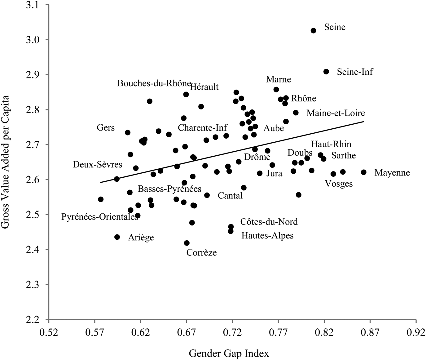
Figure 2. Scatter plot of the links between GGI and economic performance.
Source: Using data from Caruana-Galizia (Reference Caruana-Galizia2013) and Statistique Générale de la France.
Second, I tested the following equation using OLS estimators:

where i stands for the French county; k refers to the measures of gender equality, i.e., overall index and sub-indices; X i denotes the vector of the control variables; and ε i is the error term. $Economic\_Performance_i$ is captured by the Gross value added per capita measured in 1860.
X i includes controls at the county level, constructed on the basis of information from French Censuses of the 1850s, which reduce unobserved heterogeneity across counties. First, I accounted for fertility measures, namely, the child–women ratio (the number of children aged 0–5 per woman of childbearing age) and the female (median) age at marriage. Second, I controlled for infant mortality, used as a proxy for health and as a determinant of the gross potential. Third, the population density was added to equation (2) to proxy the extent of urbanization and control for dynamic gains emerging from growing cities through increasing the accumulation of human capital [Bertinelli and Black (Reference Bertinelli and Black2004)]. Fourth, I controlled for inequality in land ownership. Landowners delay the development of the industrial sector and of possible income growth because they have little interest in public schooling, given the low complementarity between land and human capital [Galor et al. (Reference Galor, Moav and Vollrath2009)]. To measure gender equality, I tested equation (2) using as alternatives the overall gender gap index, the education sub-index, the economic sub-index, and the health sub-index.
5.2 Findings
OLS estimates of equation (2) are reported in Table 6. Column 1 presents the results using the overall gender gap index as the variable of interest. A higher GGI, namely greater gender equality, was found to be significantly and positively correlated with higher economic performance. An increase of one standard deviation in the gender index was associated with an increase by 0.30 standard deviations in the gross value added per capita, at the 0.1% probability level. This positive association provided preliminary support to the theoretical predictions that empowering women benefits economic growth [Diebolt and Perrin (Reference Diebolt and Perrin2013, Reference Diebolt, Perrin, Diebolt, Carmichael, Dilli, Rijpma and Störmer2019)].
Table 6. OLS estimates of gross value added per capita
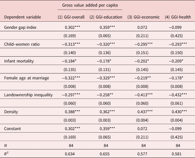
Note: OLS regressions. Dependent variable: gross value added per capita in 1860. Variable of interest: overall index (column 1); education sub-index (column 2); economic sub-index (column 3); health sub-index (column 4). Standardized β coefficients. Standard errors in parentheses. *p < 0.05, **p < 0.01, ***p < 0.001.
Source: County-level data from the Statistique Générale de la France.
The economic performance of a county can be affected by a range of additional factors likely to explain the heterogeneity observed across France. Controlling for demographic variables revealed interesting findings in line with the key predictions of unified growth models and related literature [Galor and Weil (Reference Galor and Weil1999, Reference Galor and Weil2000), Galor and Moav (Reference Galor and Moav2002), Doepke (Reference Doepke2004)]. Lower fertility rates were significantly correlated with higher economic performance (at the 0.1% percentage level). An increase of one standard deviation in the number of children per woman was associated with a decrease by 0.31 standard deviations in the gross value added. This result was in line with the idea that the demographic transition had a powerful impact on economic growth [Bloom and Williamson (Reference Bloom and Williamson1998)]. The data also confirm that health conditions, proxied by the infant mortality rate, were negatively and significantly associated (at the 5% probability level) with the economic performance of the county. According to Bloom et al. (Reference Bloom, Canning and Sevilla2004), this negative association could have occurred through lower labor productivity.
A counterintuitive result was the negative association between the female median age at marriage and the gross value added per capita. Age at first marriage is sometimes interpreted as a measure of a woman's bargaining power (Maubrigades, Reference Maubrigades, Camou, Maubrigades and Thorp2015) and is used as an indicator of female agency [Carmichael (Reference Carmichael2011)]. In the case of nineteenth-century France, as shown by Perrin and Benaim's (Reference Perrin, Benaim, Diebolt, Carmichael, Dilli, Rijpma and Störmer2019) typology, progressive counties that economically performed best were characterized by high levels of gender equality, low fertility, high enrollment rates for boys and girls, and younger age at marriage. This might mean that people could afford to marry sooner if they or their families were already prosperous. As argued by Perrin and Benaim (Reference Perrin, Benaim, Diebolt, Carmichael, Dilli, Rijpma and Störmer2019), young age at marriage in the context of nineteenth century France could also reflect the higher degree of agency (greater bargaining power in the decision-making process) that women enjoyed within the family.
As expected, counties with lower shares of landowners displayed lower gross value added per capita. An increase of one standard deviation in landownership inequality was associated with a decrease by 0.30 standard deviations in gross value added. This result confirmed the theoretical predictions of Galor et al. (Reference Galor, Moav and Vollrath2009) that inequality in the distribution of landownership played a significant role in the emergence of sustained differences in human capital formation and growth patterns across economies. My estimates also confirmed that the more densely populated areas were significantly associated with better economic performance.
The same analysis was conducted using all the sub-indices in succession. Even if the associations found for the control variables remained unchanged (with similar magnitude and significance), the sub-indices presented different results. As far as the education sub-index was concerned (column 2), the positive and significant association was confirmed.Footnote 19 An increase of one standard deviation in gender equality in education was positively and significantly associated with an increase by 0.36 standard deviations in economic performance. This positive association supports the theoretical argument that greater gender equality in human capital is beneficial for economic growth [Lagerlöf (Reference Lagerlöf2003)]. The economic and health sub-indices (columns 3 and 4, respectively), however, showed insignificant effects on economic performance.
Education appeared as a decisive factor in fostering gender equality (Table 4). The importance of education is confirmed by the coefficients presented in Table 6. Looking at the effect on economic performance of the gender gap index separately from the effects of its sub-indices, it emerged that the explanatory power of the overall index is mostly triggered by the education sub-index. This finding suggests that education is a crucial factor to improve overall gender equality and that gender equality—in particular gender equality in education—is crucial to foster economic growth.
5.3 Robustness check
The findings may have been driven by the variable chosen to measure economic performance. I therefore tested the sensitivity of the results using alternative measures of the dependent variable. I successively employed GDP per capita, manufacturing output, horse power per capita, proto-industrialization, and GVA per capita in 1886 and also in 1901, as alternative measures to economic performance.Footnote 20
The positive and significant association found in Table 6 holds for all the alternative measures of economic performance. These results confirm the existence of a robust and significant association between gender equality and economic growth (Table 7).
Table 7. Alternative measures of economic performance

Note: OLS regressions. Dependent variable: gross domestic product per capita (column 1); manufacturing output (column 2); horse power per capita (column 3); proto-industrialization (column 4); gross value added per capita in 1886 and 1901 (column 5 and 6, respectively). Variable of interest: overall index (in each specification). Control variables: same controls as the ones used in Table 6. Standardized β coefficients. Robust standard errors in parentheses *p < 0.05, **p < 0.01, ***p < 0.001.
The analysis conducted in section 5 empirically confirmed the close association between gender equality and economic growth. It also showed the usefulness of accounting for the multiple dimensions of gender equality. My results suggest that efforts to foster gender equality and boost economic growth need to be made within the overall spectrum of gender equality. As shown in the analysis conducted in sub-section 4.2, education appeared incremental for doing so.
6. Conclusion
The primary contribution of this paper is the construction of a gender gap index at the historical level. This paper is the first attempt to capture the multi-dimensional aspects of gender equality in the past—during a critical period of France's process of economic and demographic development. My ambition with the construction of such an index was to provide a comprehensive measure of gender equality, easily comparable with other variables, i.e., economic, demographic, or cultural, from a historical perspective, which could also easily be extended to incorporate dynamic components and be generalizable to other countries.
Based on an original county-level dataset of 86 observations in the mid-nineteenth century stemming from the Statistique Générale de la France, I built an index quantifying the size of the gap between men's and women's achievements in three critical areas: economic participation and opportunities, educational attainment, and health and survival. The county comparisons enabled me to identify the strengths and weaknesses of the French regions in closing the gender gap. The geographical distribution of the index highlighted the existence of a great heterogeneity across regions. In particular, it showed that the counties located on the Northern part of France performed best.
The analysis of the determinants of the gender gap contributes to revealing some specific characteristics of the regions that were performing the best. Counties characterized by greater education for boys and girls, dynamic industries employing high shares of female and male workers, and those offering women access to well-paid jobs displayed higher gender equality. Additional results showed that counties with higher shares of married women displayed lower scores on the various dimensions of gender equality. Further inquiry conducted on family structures showed that the types of nuclear family displayed greater gender equality than the types of extended family.
The third contribution of the paper was to investigate the association between gender equality and economic growth in the past. The analysis showed a positive and significant association between gender equality and economic growth. The results hold regardless of the variable used to measure economic performance. French counties that have succeeded best at closing their gender gap have displayed better economic performance and exhibited lower fertility rates. This association is consistent with the literature stating that empowering women affected fertility in various ways [see Caldwell (Reference John1981), and Brée and de la Croix (Reference Brée and de la Croix2019) for an empirical investigation of the French town of Rouen in the seventeenth and eighteenth centuries] and is beneficial to economic growth [see Kabeer and Natali (Reference Kabeer and Natali2013), Cuberes and Teignier (Reference Cuberes and Teignier2014), and Klasen and Santos Silva (Reference Klasen and Santos Silva2018), for exhaustive reviews of the literature], and confirms the theory developed by Diebolt and Perrin (Reference Diebolt and Perrin2013, Reference Diebolt, Perrin, Diebolt, Carmichael, Dilli, Rijpma and Störmer2019) according to which female empowerment in the direction of greater equality underlies the demographic transition and triggers sustained economic growth.
Additionally, the analysis shows that the overall index—which encompasses the wider variety of gender indicators—and the education sub-index capture many more variations in economic performance than the economic and health sub-indices. Taken together, the analyses of the determinants of gender equality and the effect of gender equality on economic growth have wide political implications. Our results endorse the importance of accounting for the multidimensional aspects of gender equality in economic growth. They suggest that, to be more efficient, policies in favor of economic development must rely on an approach that fosters gender equality on all its many dimensions. Policies must account for the wide range of determinants that affect gender equality, e.g., girls' and boys' education, women's access to resources and opportunities, but also culture and social norms embedded in the territory, as reflected by the family structures, that can profoundly and durably affect individuals' behaviors with regards to gender equality.
To conclude, it is important to acknowledge that the empirical results of this paper are limited to simple correlations. Further analysis is required to determine the direction(s) of causation between the various factors that were integrated and discussed in the current analysis. In any case, the current investigation may not capture the full complexity of the relationships of interest and further research on this point is needed. The 1850s gender gap index is a first step toward the generalization of the index to longer time periods—such as would enable us to account for the dynamic evolution of gender equality over time—and toward the extension of the index to other countries from a comparative perspective. The ultimate ambition of this work is to deepen the understanding of economic and demographic processes and maybe bring elements of answers to some of the most persistent puzzles underlying the long-run development process.
Acknowledgements
I am grateful to the anonymous referees for their valuable comments and suggestions. I also thank the participants of the following conferences and seminars for their feedbacks and comments on an earlier version of the paper: Macrohistory Seminar, University of Bonn; XVIIth World Economic History Congress, Kyoto; European Historical Economics Society Conference, Pisa; Workshop on Women in Changing Labor Markets, Lund; 24th IAFFE Annual Conference—Gender Equality in Challenging Times, Berlin; Odense FRESH Meeting; Debunking Austerity: Towards Alternative Economic Policy Scenarios, SSSUP, Pisa. The paper has also benefitted from precious feedbacks from Audrey-Rose Menard.
Appendix A
The gender gap index
The data used to construct the index were mainly extracted from books published by the Statistique Générale de la France (SGF) on population and demographic and public education censuses, between 1800 and 1925. Almost all the data were available for 86 counties.
Variables
• Female (Male) in industry, in 1851. Number of women (men) employed in manufacturing over total number of women (men) aged 15–60. Manufacturing refers to all types of industry: textiles, the metals sector, and other factories (food, wood, construction, etc.).
• Female (Male) in agriculture, in 1851. Number of women (men) employed in agriculture over total number of women (men) aged 15–60. Agriculture refers to all positions within the agricultural sector: owners, farmers, sharecroppers, and others.
• Female (Male) wages in industry, in 1861. Average of female (male) workers' wages in francs in different industries proportionally to the weight of females (males) in each industry for each department. Manufacturing refers to all types of industry: textiles, the metal sector, and other factories (food, wood, construction, etc.)
• Female (Male) wages in agriculture, in 1852. Average of female (male) farm workers' wages in francs for one working day in the agricultural sector.
• Female (Male) literacy rate, in 1854. The literacy rate consists of the number of individuals able to read and to write over total population. 1856–66
• Girls' (Boys') enrollment rate, in 1850. Number of girls (boys) enrolled in public primary schools over the total number of girls (boys) aged 5–15.
• Girls' (Boys') public primary schools, in 1850. Number of public primary schools dedicated to girls (boys).
• Life expectancy at age 0, in 1856. The life expectancy is the expected (in the statistical sense) number of years of life remaining at a given age (here at age 0)—calculated by constructing a life table.
• Female (Male) live births in 1851. Number of female (male) living births.
• Female (Male) mortality rate in 1851. Number of women (men) who died per 1,000 living women (men).
Table A.1. Structure of the 1850s gender gap index


Figure A.1. Administrative France.
Source: https://www.ign.fr/institut/ressources-pedagogiques#Fonds2
Note: The names of several départements have changed over time. Before 1970, the Alpes-de-Haute-Provence was called Basses-Alpes; before 1941, the Charente-Maritime was known as the Charente-Inférieure; before 1955, the Seine-Maritime was entitled Seine-Inférieure; and before 1968, Paris, Hauts-de-Seine, Seine-Saint-Denis, and Val-de-Marne composed the Seine, while Yvelines, Essonne, and Val-d'Oise together were known as the Seine-et-Oise.
Table A.2. Ranking and scores: overall index

Table A.3. Ranking by sub-index—economic opportunity and participation

Table A.4. Ranking by sub-index: educational attainment
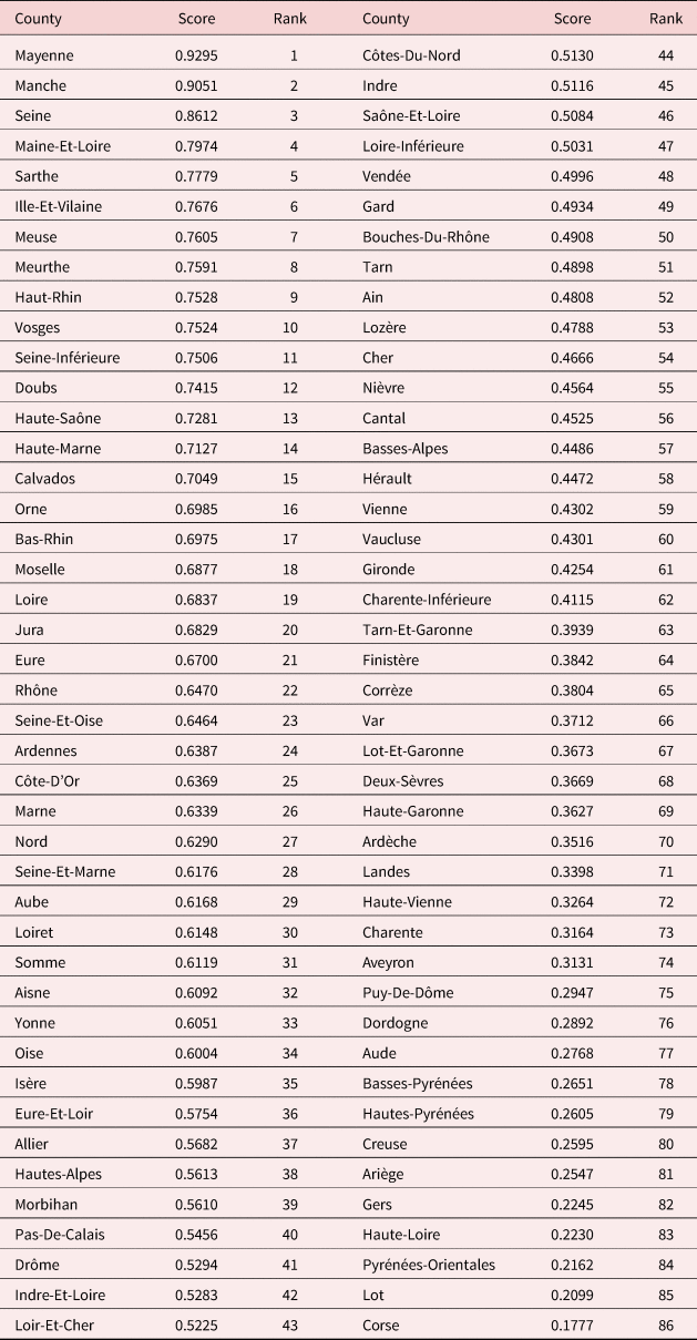
Table A.5. Ranking by sub-index: health and survival


Figure A.2. Sub-index scores in relation to gender gap index scores.

Figure A.3. Radar chart of regional profiles.
Appendix B
Empirical analysis
The data used to conduct the empirical analysis were mainly extracted from books published by the Statistique Générale de la France (SGF) on population, demographic, industrial, agricultural, and educational censuses, between 1800 and 1925. Almost all data were available for 86 counties.
Variables
• Density. Number of individuals per km2, 1851.
• Urban residents. Number of individuals living in towns with more than 2,000 inhabitants in total, 1851.
• Share married women. Number of married women per women of marriageable age (15+), 1851.
• Individuals per house. Number of individuals living per house, 1852.
• Child–women ratio. Number of children aged 0–5 per woman of childbearing age (15–45), 1851
• Infant mortality. Mortality rate at age 0 (from life table), 1851.
• Female age at marriage. Women's mean age at marriage, 1855.
• Landownership inequality. Number of monetary contributions above 300 francs over land ownership per total number of monetary contributions over land ownership, 1835.
• Gross value added per capita, in 1860, 1886, 1901. From Caruana-Galizia (Reference Caruana-Galizia2013).
• GDP per capita. Value added in agriculture, industry, a tertiary sector per capita (in thousands), 1860. From Combes et al. (Reference Combes, Lafourcade, Thisse and Toutain2011)
• Manufacture output. Manufacturing output per capita, 1861
• Horse power per capita. Horse power of steam engines per capita (in 10,000), 1861.
• Proto-industrialization. Number of steam engines per capita (in thousands), 1861.
• Family structure. Stem family (famille souche + famille souche imparfaite); Intermediary/Communitarian family (famille communautaire + zone atlantique intermédiaire + famille nucléaire à corésidence du nord + formes nucléaires imparfaites et communautaires bretonnes); Cooperative (famille nucláire patrilocale égalitaire); Nuclear absolute family (famille hypernucléaire de l'Ouest); Nuclear egalitarian family (famille nucléaire égalitaire). See Le Bras and Todd (Reference Le Bras and Todd2013).
Table B.1. Summary statistics of the variables


 Open access