


Introduction
Social network analysis is a method to investigate relations and interactions between actors in groups (Wasserman and Faust, Reference Wasserman and Faust1994; Newman, Reference Newman2010). This is not limited to studies on humans and has been increasingly applied to animal behaviour in recent years (Lusseau and Newman, Reference Lusseau and Newman2004; Croft et al., Reference Croft, James, Ward, Botham, Mawdsley and Krause2005; McCowan et al., Reference McCowan, Anderson, Heagarty and Cameron2008; Drewe et al., Reference Drewe, Madden and Pearce2009; Hinton et al., Reference Hinton, Bendelow, Lantz, Wey, Schoen, Brockett and Karubian2013; Büttner et al., Reference Büttner, Czycholl, Mees and Krieter2019), as the behaviour of group-housed animals is affected by the behaviour of other pen mates as well (Makagon et al., Reference Makagon, McCowan and Mench2012). Thus, the group structure is important for the understanding of the individual's behaviour and social network analysis is a useful method to analyse it (Krause et al., Reference Krause, Croft and James2007). In a network, the animals are represented by nodes that are connected by edges that represent the interactions between the animals (Asher et al., Reference Asher, Collins, Ortiz-Pelaez, Drewe, Nicol and Pfeiffer2009). These interactions can be undirected, for example sharing the same sleeping place, or directed, if there is a definite initiator and receiver, for example grooming or fighting. The resulting edges are either bidirectional connecting both nodes with each other or unidirectional connecting only the initiator with the receiver but not inversely. The edges can be either unweighted, i.e. present or absent, or they can be weighted, if for example the frequency of the interaction is important for the further analysis (Wasserman and Faust, Reference Wasserman and Faust1994; Wey et al., Reference Wey, Blumstein, Shen and Jordán2008; Croft et al., Reference Croft, Madden, Franks and James2011). Several network parameters at network and node-level have been developed, providing a standardized way to describe the group structure or the node's position within this group (Wasserman and Faust, Reference Wasserman and Faust1994; Newman, Reference Newman2010). Using these parameters, studies of the changing group structure after the removal of animals or the addition of animals to the group (Williams and Lusseau, Reference Williams and Lusseau2006) or at different age levels (Büttner et al., Reference Büttner, Scheffler, Czycholl and Krieter2015) are possible. However, social network analysis faces problems of extensive data acquisition, thus different studies investigated the influence of missing data or adding false data on real networks or theoretical networks (Zemljič and Hlebec, Reference Zemljič and Hlebec2005; Borgatti et al., Reference Borgatti, Carley and Krackhardt2006; Kim and Jeong, Reference Kim and Jeong2007; Frantz et al., Reference Frantz, Cataldo and Carley2009; Voelkl et al., Reference Voelkl, Kasper and Schwab2011; Wang et al., Reference Wang, Shi, McFarland and Leskovec2012; Büttner et al., Reference Büttner, Salau and Krieter2018). In the case of network analysis on animals, they often rely on behavioural observations to obtain the requested information on the animals. During these observations, different problems may cause errors in the datasets altering the resulting networks. For example, different interpretations of the ethogram or distraction and weariness due to extensive workload can lead to missed events.
Thus, the aim of the current study was to analyse the effect of missed events on the robustness of animal networks. Therefore, a model data set of networks based on real tail-biting behaviour observations in pigs was used as a gold standard and two datasets were compared to it, one dataset of real networks and one dataset of simulated networks. The first dataset consisted of the observations of the same pigs but analysed by three other observers. The second dataset consisted of random samples of the gold standard dataset to simulate missed events at fixed error rates. It was investigated whether deviations of real observers are comparable to missing events at random and whether the robustness of sampled networks is affected by other factors apart from the error rate. With this knowledge, it is possible to choose appropriate observation periods and to acquire valid data.
Materials and methods
Animals and experimental design
The video footage used in the current study was recorded on the agricultural research farm ‘Futterkamp’ of the Chamber of Agriculture of Schleswig-Holstein in Germany from November 2016 until April 2017. There, 144 crossbreed piglets (Pietrain × (Large White × Landrace)) were housed together in six conventional pens with 24 individually marked piglets per pen after an average suckling period of 28 days. For 40 days, the pens were each video recorded by one AXIS M3024-LVE Network Camera produced by Axis Communications. The tail lesions of the piglets were scored twice a week according to the ‘German Pig Scoring Key’ (German designation: Deutscher Schweine Boniturschlüssel) (Anonymus, 2016). When at least one large tail lesion (larger than the diameter of the tail) had been documented on a scoring day, the video footage of the previous 4 days was analysed for the tail-biting behaviour of the piglets. This was analysed using continuous event sampling during the light hours (6:00–18:00 h) resulting in 288 h of video observation. Because of the fixed camera angle, the chewing movement of the biting pig could not be seen for every tail-directed behaviour on the video footage. Therefore, tail-biting behaviour was defined as manipulating, sucking or chewing on a pen mate's tail (Zonderland et al., Reference Zonderland, Schepers, Bracke, den Hartog, Kemp and Spoolder2011). The initiator, receiver and the time of each tail-biting behaviour event was recorded.
Video analysis
The video analysis was carried out by four trained observers. Beforehand, every observer had to analyse the tail-biting behaviour in a test video to determine the interobserver reliability using Cohen's κ (Cohen, Reference Cohen1960). This video consisted of short clips showing a group of pigs in which one pig may or may not have performed tail-biting behaviour. If the interobserver reliability was too low (Cohen's κ < 0.7), the observers had to resume the training. The test video analysis was repeated throughout the study to check for changes in the interobserver reliability and to test the intraobserver reliability. For this purpose, a fixed number of clips remained in the test video, the remaining clips were exchanged and all clips were put in a random order. Again, if the inter- or intraobserver reliability was too low, the observer had to resume the training.
True v. observer – comparison of different observers
The reliability of the test videos proved to be good (Cohen's κ: 0.9 ± 0.08 (Mean ± standard deviation)), but still differences between the observers in the actual video analysis became obvious at some point. The intraobserver reliability of the test videos was calculated and observations were scanned for mistakes by the supervisor who was responsible for the training. The observer with the highest intraobserver reliability (Cohen's κ: 0.8 ± 0.10) and least missed events was chosen as a reference and was assigned to complete the video observations. Therefore, the video observation of the whole observation period was done by one observer. For the current study, it was assumed that all events actually happened and no events were missed by this observer. Thus, these tail-biting behaviour observations formed the true dataset. The other three observers analysed only some days of the observation period and their tail-biting behaviour observations formed the observer datasets, which were later compared to the true dataset.
True v. sampled – comparison of different error rates
For a better understanding of the extent of deviations between observers and its consequences, the true dataset was used to simulate missing observations with a fixed error rate. Therefore, random samples were drawn from the true dataset containing 1/10–9/10 of the tail-biting behaviour events. Thus, a sample containing 1/10 of the initial events had 9/10 of missing observations. All samples were drawn evenly throughout the observation period and all six pens. At each sampling rate, the sampling was iterated 1000 times. Therefore, there were 9000 samples which formed the sampled datasets which were later compared to the true dataset, as well.
Network analysis
Networks consist of nodes and edges, where an edge connects the initiating node with the receiving node. The current study used tail-biting behaviour observations as a basis for the networks. Since tail-biting behaviour has a clear initiator and receiver and the frequency of the interaction between the pigs is known, the edges are directed and weighted to represent the tail-biting behaviour. To build networks out of the true, observer and sampled datasets, the four analysed days of each pen were divided into time windows and the tail-biting behaviour was summed up within these time windows. An example is illustrated in Fig. 1. To analyse the effect of different lengths of observation periods, time windows of lengths 0.5, 1, 3, 6 and 12 h were chosen. To do this, the 12 h of observation per day were evenly divided into subsets without overlapping for each length. This resulted in 43 time windows (24 × 0.5, 12 × 1, 4 × 3, 2 × 6, 1 × 12 h) per day and the tail-biting behaviour was summed up within each time window separately to generate independent networks. All networks contained 24 nodes but differed in their density, i.e. the number of present edges divided by the number of possible edges in the network, depending on the time window or sampling rate.
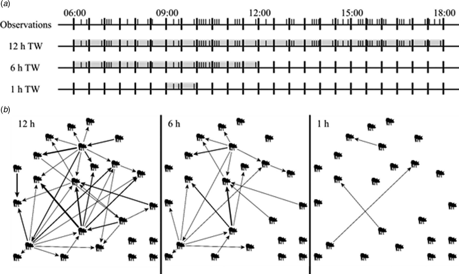
Fig. 1. (a) Example of 12 h of observation of one pen. Each I represents a tail-biting observation. Illustrated are the tail-biting observations that are included in a 12 h time window (TW) (06:00–18:00), in a 6 h TW (06:00–12:00) and an 1 h TW (09:00–10:00). (b) Graphs of the resulting tail-biting networks of the 12 h TW, 6 h TW and 1 h TW. The pigs display the nodes and the arrows display the edges pointing from the initiating to the receiving node, representing tail-biting observations. The thickness of the arrows displays the weight, i.e. the frequency, of an edge. The more frequent an edge was present, the thicker this edge is displayed.
There are several node-level centrality parameters that can be calculated for each node in the resulting networks individually (Wasserman and Faust, Reference Wasserman and Faust1994; Newman, Reference Newman2010). The centrality parameters weighted in-degree, weighted out-degree, weighted ingoing closeness centrality, weighted outgoing closeness centrality and the weighted betweenness centrality were used in the current study. The degree of a node is the number of nodes that have a connection to this node. If a pig was not involved in tail-biting behaviour at all, i.e. had no connections to other nodes within a given time window, it was considered an isolated node. In a directed network, the degree is divided into the in-degree, i.e. the number of nodes with a connection to this node, and the out-degree, i.e. the number of nodes this node has a connection to. The weighted in-degree and the weighted out-degree of a node are the sum of all ingoing edges or outgoing edges, respectively. In the context of tail-biting behaviour, it is the number of initiated or received tail-biting behaviour events. Two nodes can also be connected in an indirect way, if they are both connected to a third node or if there is a path over several other nodes. The closeness centrality of a node is the reciprocal mean path length needed to reach all connected nodes in this network. Similar to the degree, it is divided into the ingoing closeness and the outgoing closeness, if the network is directed. There, the ingoing closeness of a node is the reciprocal mean path length of all connected nodes to reach this node and the outgoing closeness centrality of a node is the reciprocal mean path length of this node to reach all other connected nodes. In an unweighted network, the path length of every edge is one. If the edges in a network are weighted, a high edge weight represents a frequent interaction between the nodes. Therefore, if an edge with a high weight connects two nodes, they are considered to be closer together and the edge is ‘easier’ to pass. In order to retain this relation for the calculation of the centrality parameters, the inverse edge weight is used as the path length. It is also possible for two nodes to be connected by more than one path as well. Then, the shortest path is the path including the fewest edges. The betweenness centrality is the number of shortest paths between all other nodes going through this node divided by the number of all shortest path between the other nodes. In a directed network, the betweenness centrality considers the direction of the edges. If the edges are weighted, the path length of an edge is the inverse edge weight, as it is for the weighted closeness centrality.
For each time window in all datasets (true, observer and sampled), the tail-biting behaviour was used to build a network and the centrality parameters were calculated for each node individually. The calculation of the network parameters were carried out using the Python module NetworkX (Hagberg et al., Reference Hagberg, Schult and Swart2008) and the network graph was created using yEd (yWorks GmbH 2021).
Statistical analysis
To analyse the robustness of the centrality parameters, all five centrality parameters of the erroneous networks (observer and sampled) were compared to the centrality parameters of the respective true network using different measurements of accuracy. Comparisons were only carried out between networks of the same pen, day and time window. For example, a sampled network of pen 2 on day 1 using the tail-biting behaviour of the time window 12:00 to 13:00 was compared to the true network of pen 2 on day 1 using the tail-biting behaviour of the time window 12:00 to 13:00. The current work was oriented towards the study of Borgatti et al. (Reference Borgatti, Carley and Krackhardt2006), in which they used the stability of the ranking order as a criteria of accuracy. However, because of tied ranks in all three sorts of our networks, the measurements of accuracy had to be modified. The first measure ‘Overlap Top 1’ is the accuracy to choose the animal(s) in the highest rank based on an erroneous network correctly. It was defined as the overlap between the set of nodes in the highest rank of the true network and the set of nodes in the highest rank of the erroneous network. It is computed as $[ {U\cap V} ] /[ {U\cup V} ] , \;$ where U is the set of nodes in the highest rank of the true network and V is the set of nodes in the highest rank of the erroneous network. The second measure ‘Overlap Top 3’ is the accuracy to choose the animals in the top three ranks based on an erroneous network correctly. It was defined as the overlap between the set of nodes in the top three ranks of the true network and the set of nodes in the top three ranks of the erroneous network independent of the order within these ranks. It is computed equivalent to ‘Overlap Top 1’. The last measure ‘R 2’ is the square of the Spearman correlation coefficient between the true and erroneous networks to analyse the changing of the ranking order, i.e. the group structure, in the whole pen. It can be interpreted as the proportion of variance in the ranking order of the true network accounted for by the ranks of the erroneous network. Apart from tied ranks, there was another problem, especially with less dense networks. The number of isolated nodes in a network increased with a decreasing number of edges. However, if a node has no edges, it cannot be affected by random edge removal and therefore the centrality parameters of isolated nodes cannot change. This could falsely alter the accuracy measurements in a positive direction. To prevent this, nodes, which were isolated in the true networks, were not included in the calculation of the accurate measurements. Furthermore, sparse networks were excluded, in which all nodes were in the top three ranks of the sampled network, from the calculation of ‘Overlap Top 3’, because this could falsely alter the accuracy scores as well. The three accuracy measurements were used to compare the centrality parameters of the observer and sampled networks with their respective true network. ‘Overlap Top 1’ measures the proportion of correctly chosen animals in the first rank, ‘Overlap Top 3’ measures the proportion of correctly chosen animals in the first three ranks and ‘R 2’ measures the stability of the ranking order in the whole pen. The statistical software package SAS 9.4 (SAS® Institute Inc., 2013) was used for the analysis.
For the interpretation of the accuracy scores of a centrality parameter, it was tried to give a rough estimate of what is good accuracy. Assuming a stable ranking order indicates that there are only few changes in network structure, high accuracy scores indicate robust centrality parameters. However, there are no established thresholds to distinguish between a good, moderate or bad accuracy for the measurements of accuracy used in the current study. In a more general context, Martin and Bateson (Reference Martin and Bateson2012) stated that a Spearman correlation coefficient of 0.7 and greater is a marked relationship and a Spearman correlation coefficient of 0.9 and greater is a very dependable relationship. Applying these thresholds to the squared Spearman correlation coefficient, ‘R 2’ accuracy scores of 0.49 and greater can be interpreted as good results and ‘R 2’ accuracy scores of 0.81 and greater can be interpreted as very good results regarding the group structure. Because the accuracy scores of the ‘Overlap Top 1’ and ‘Overlap Top 3’ measurements tend to be in the same range as the accuracy scores of ‘R 2’, the thresholds of ‘R 2’ were applied as well to interpret the accuracy of correctly choosing the animal in the highest rank or the highest three ranks respectively.
Results
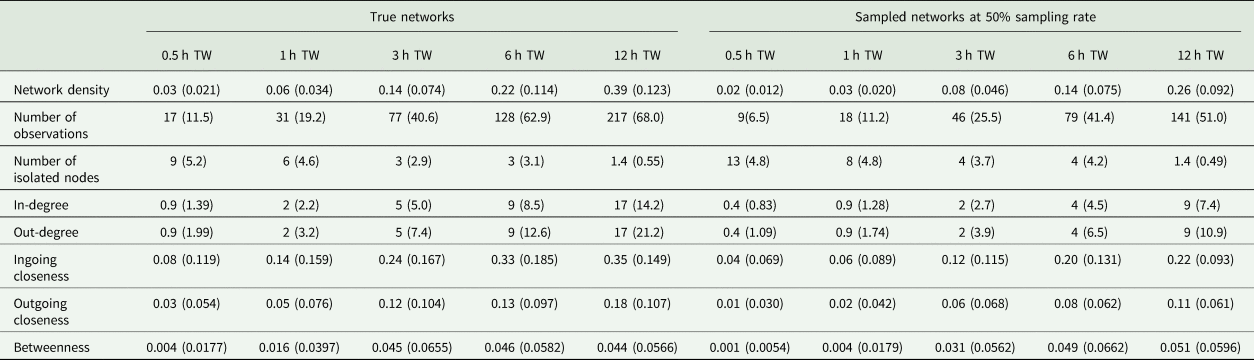
During the observation period, there were 217 ± 68.0 (mean ± standard deviation) tail-biting behaviour events per day and pen in the true dataset. All networks consisted of 24 nodes but varied in their number of edges depending on the tail-biting activity and time window used. In case of the sampled networks, the sampling rate affected the number of edges as well. The mean and standard deviation of the network density, number of isolated nodes and the centrality parameters of the true networks and the sampled networks (exemplary at a sampling rate of 5/10) can be seen in Table 1. For the accurate measurements of ‘Overlap Top 1’ and ‘Overlap Top 3’, all animals were ranked in the first rank or in the first three ranks in 3 ± 10.2% or 23 ± 29.3%, respectively, of the sampled networks. Thus, these networks were excluded from the calculation.
Table 1. Mean (standard deviation) of the network density, number of observations, number of isolated nodes and the weighted centrality parameters for all true networks and all sampled networks exemplary at 50% sampling rate regarding the time window (TW)
True v. observer – comparison of different observers
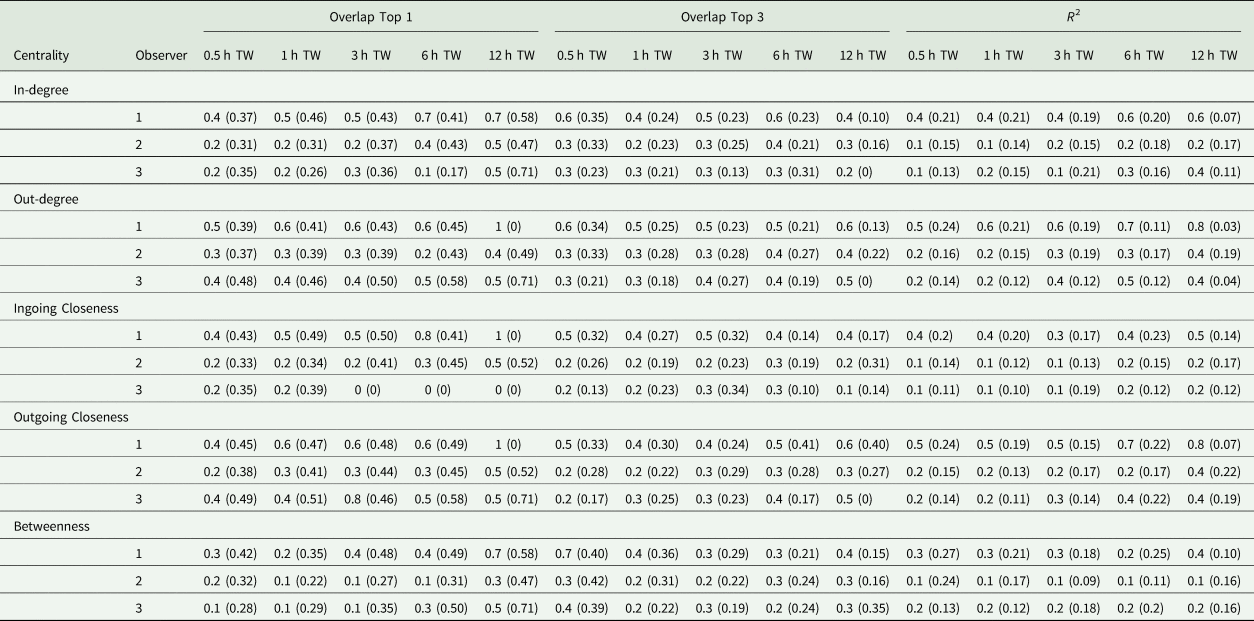
The first step of the current study was to compare the observer datasets with the true dataset. Comparing the number of documented tail-biting behaviour events, the observers documented 68 ± 20.3% (mean ± standard deviation) fewer events than the reference (observer 2: 30 ± 5.3%, observer 3: 77 ± 9.7%, observer 4: 75.1 ± 0.52%). The accuracy scores of the three observers compared with the true dataset are shown in Table 2. Most of the accuracy scores were smaller than the thresholds of 0.49 or 0.81 mentioned. The accuracy scores differed according to the time window used, the accurate measurement and the analysed centrality parameter, but did not always show a clear trend. For the accuracy measurement ‘R 2’, larger time windows yielded higher accuracy scores and for the ‘Overlap Top 1’, this was also true for most cases but was not the case for the ‘Overlap Top 3’. Especially the ‘Overlap Top 1’ and ‘Overlap Top 3’ accuracy scores for the 30 min time window showed contrary behaviour, as they yielded higher scores in some cases compared to larger time windows. Comparing the measurements of accuracy, ‘Overlap Top 1’ yielded the highest accuracy scores most of time, but there was variability depending on the other parameters as well. For the different centrality parameters, in most cases, the outgoing centrality parameters (weighted out-degree, weighted outgoing closeness centrality) yielded higher accuracy scores compared to ingoing centrality parameters (weighted in-degree, weighted ingoing centrality parameters), whereas the betweenness centrality yielded the lowest accuracy scores. Overall, observer 2 provided the highest accuracy scores and exceeded the mentioned thresholds more often than the other two observers.
Table 2. Mean (standard deviation) (Overlap Top 1 and Overlap Top 3) or median (standard deviation) (R 2), respectively, of accuracy scores of observer networks compared to the true networks regarding the weighted centrality parameters and time window (TW)
True v. sampled – comparison of different error rates
The second step of the current study was to compare the sampled datasets with different error rates with the true dataset. The results of the accurate measurements for all centrality parameters, time windows and sampling rates are shown in Fig. 2. It presents plots of the results of all used centrality parameters of the sampled networks as a function of sampling rate for all used time windows and accuracy measurements. In Fig. 2a, the mean accuracy scores for the ‘Overlap Top 1’ of the weighted in-degree of all time windows start around 0.3 at a sampling rate of 1/10 and increase more or less linearly to 1.0 at a sampling rate of 10/10. There were small differences between the time windows with larger time windows having better accuracy scores, but these differences became smaller for higher sampling rates. This is similar for the ‘Overlap Top 3’, but here, the overall differences between the time windows were smaller. On the other hand, the curves of the accuracy scores of ‘R 2’ varied between the time windows. The curve of the 30 min time window starts at 0.14 with a linear increase until 1.0 at a sampling rate of 10/10. However, the curve of the 12 h time window starts at 0.46 with a steep increase for the lower sampling rates and a slow increase for the higher sampling rates until it reaches 1.0 at a sampling rate of 10/10 as well. The other time windows ranged in between relatively to their size.
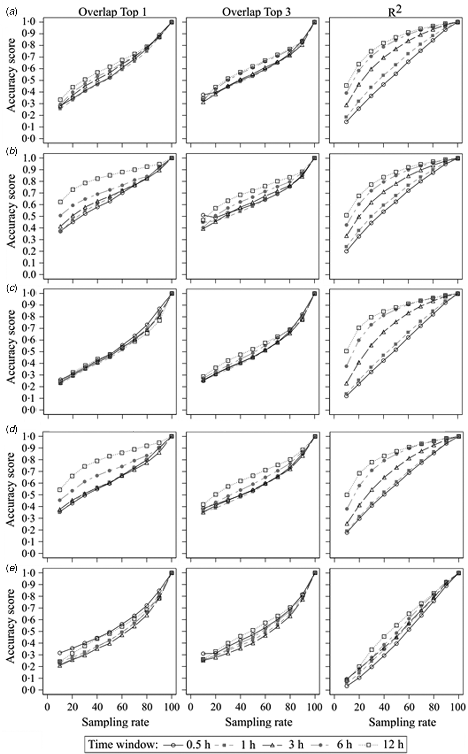
Fig. 2. Sampled networks compared to the true networks; accuracy scores of (a) the weighted in-degree, (b) the weighted out-degree, (c) the weighted ingoing closeness centrality, (d) the weighted outgoing closeness centrality and (e) the weighted betweenness centrality according to the sampling rate and measured by ‘Overlap Top 1’, ‘Overlap Top 3’ and ‘R 2’ regarding the different time windows.
Generally, all accuracy scores increased with increasing sampling rate independent of used centrality parameter, time window or accuracy measurement with only one exception (‘Overlap Top 3’ of the weighted out-degree using 0.5 h time window: accuracy score of 0.51 at a sampling rate 1/10 v. 0.49 at a sampling rate of 2/10). But with regard to the mentioned thresholds of accuracy, in most cases there were differences between the centrality parameters, time windows or accuracy measurement. If there were differences between the time windows, larger time windows resulted in greater accuracy scores compared to smaller time windows. The only exceptions were the ‘Overlap Top 3’ measurement of very sparse networks (due to small time window and/or small sampling rate), for which sparser networks yielded greater accuracy scores. Mostly, the accuracy scores measured with the squared Spearman correlation coefficient were greater than the accuracy scores of ‘Overlap Top 1’ or ‘Overlap Top 3’. The exception was again the ‘Overlap Top 3’ measurement for sparse networks, which differed as mentioned before. For the outgoing centrality parameters (weighted out-degree and weighted outgoing closeness), the accuracy scores of ‘Overlap Top 1’ were greater than ‘Overlap Top 3’. These differences were greater for larger time windows. For the ingoing centrality parameters (weighted in-degree and weighted ingoing closeness), larger sampling rates yielded greater accuracy scores for ‘Overlap Top 1’, while smaller sampling rates yielded greater accuracy scores for ‘Overlap Top 3’, but these differences were smaller compared to the outgoing centrality parameters. Overall, the results demonstrate that outgoing centrality parameters had higher accuracy scores compared to ingoing centrality parameters. Moreover, ‘local’ centrality parameters (weighted in-degree and out-degree) had higher accuracy scores compared to ‘global’ centrality parameters (weighted ingoing and outgoing closeness, weighted betweenness), with the weighted betweenness centrality yielding the lowest accuracy scores.
Discussion
The current study analysed the robustness of centrality parameters by comparing a true dataset of tail-biting behaviour with erroneous datasets using three different measurements of accuracy. In the first step, the true dataset was compared to the datasets of three real observers, which analysed the same video footage. In the second step, random samples of the true dataset were drawn to analyse the robustness at a fixed error rate. The accuracy scores differed considering the time window, accuracy measurement, centrality parameter and, in case of the sampled datasets, sampling rate.
Accuracy scores
The thresholds for interpreting the accuracy scores mentioned were proposed as rough estimations of what is good accuracy. However, as there are no standard thresholds for ‘Overlap Top 1’ and ‘Overlap Top 3’, it is always important to consider the context of the requested information and to choose an appropriate threshold for it. For example, selecting one animal with the highest number of contacts for further observations may be able to handle a low accuracy without any problems, as the animal with the second or third highest number of contacts may be suitable for the observations just as well if it is chosen by mistake. However, selecting and removing the most central animals between two subgroups to contain the spread of an infection may be a situation in which it would be crucial to guarantee high accuracy, otherwise the measure would fail (Borgatti et al., Reference Borgatti, Carley and Krackhardt2006).
True v. observer – comparison of different observers
Although all the observers achieved good to very good interobserver reliability results in the training video analysis before and during the actual analysis, the comparison of the resulting networks between the other observers and the true dataset yielded mostly poor results. Assuming the observers missed events at random, as in the ‘True v. Sampled’ comparison, the mean sampling rate would have been about 23/100 (observer 2: 40/100, observer 3: 13/100, observer 4: 18/100), thus they would have missed 77/100 of the actual events (observer 2: 60/100, observer 3: 87/100, observer 4: 82/100). This is more than the actual difference of documented events because the events were probably not missed at random. Since there were 24 pigs per pen, events could have happened at the same time, which could have resulted in systematic mistakes. For example, the observers could have focused on the fast movements in the foreground, while overseeing tail-biting events in the lying area in the background. Or they could have focused on individual pigs which had performed tail-biting behaviour before. These biased observations might have led to worse accuracy scores than missing events at random. Thus, only one observer achieved very good results for larger time intervals for some centrality parameters.
The observers were only allowed to start or continue the video analysis if they had achieved good results in the training. Therefore, they were probably focused during the test situation, but during the actual video analysis weariness and distraction were more likely to increase over time, leading to missed events. To detect these deviations caused by distraction, parts of the actual video footage could be used as a testing sequence and allocated to all observers without labelling them as testing videos. This way, the observers would analyse it in the same situation and with the same focus as the actual analysis.
The results illustrate problems of carrying out observations with multiple observers, which is often done to speed up data acquisition. Although the observers in the current study were all trained and tested in the same way, the comparison of the observer datasets to the true datasets produced poor results. Having only one observer to analyse the video footage takes more time to complete observations, but it ensures a dataset without the potential deviation of different observers. However, this alone does not guarantee the correctness of a dataset. For the current study, the true dataset was only accepted for further investigation, after screening and confirming the observed events on a random basis and validating the intraobserver reliability. A validation of comparability of different observers is recommended for future studies as well, at least on a random basis, to ensure valid results.
True v. sampled – comparison of different error rates
The random edge removal used in the current study simulates observers missing events during the video analysis. But missing events does not necessarily happen at random. For example, the observers could be focused during most of the analysis, but in the last 20 min before a break they become unfocused and start to miss events. Or they recognize a pig performing a lot of tail-biting behaviour and monitor this pig closely, while overlooking less active pigs. The edge removal of random sampling is evenly distributed throughout the day and between the pigs. Thus, the ranking order does not change that much on average as the centrality parameters are altered more or less evenly as well. Comparing the results of the observer datasets with the sampled datasets shows that the observer datasets yielded worse accuracy scores at the same percentage of missed events. Therefore, bias in sampling or observation leads to worse accuracy. Furthermore, missing events is not the only error possible in video analysis. Misidentification of the involved pigs or misclassification of the behaviour do happen as well but these were not simulated in the current study. The study of Wang et al. (Reference Wang, Shi, McFarland and Leskovec2012) studied both false negative and false positive edges (misclassification) in networks and found that false-negative edges affect the accuracy more than false-positive edges.
Time window
The effect of the different length of time windows can be explained with the number of observations underlying the respective time window of the true network as in general the number of observations increased with larger time windows. With more observations, there can be more redundant observations between the same pigs. If one of the redundant observations between two animals is missing in the erroneous network, the effect on the accuracy is smaller than missing the only existing observation between two pigs. In the first case, only the edge weight is reduced by one, but in the second case the entire edge is missing. Thus, larger time windows provide more redundancy that can compensate for missing observations. This corresponds to the study of Voelkl et al. (Reference Voelkl, Kasper and Schwab2011), who found generally more stable results for datasets with more than 100 observations, and Zemljič and Hlebec (Reference Zemljič and Hlebec2005), in which denser networks yielded more stable measures of centrality. In the study of Borgatti et al. (Reference Borgatti, Carley and Krackhardt2006), increasing the network density, thus the number of edges, reduced the accuracy. But they resampled unweighted edges without any redundancy. Therefore, the edges in the observed network could only be present or absent. Thus, denser networks provided for more edges being removed at the same sampling rate thereby making greater changes in the network as a whole and reducing the accuracy of the centrality parameters.
There were some exceptions for the ‘Overlap Top 3’ measurement, in which the time window of 0.5 h yielded better accuracy scores than larger time windows. Because these networks were quite sparse, i.e. having only few observations, there were a lot of tied ranks in the first three ranks of the sampled network. Therefore, there was a high probability that the set of nodes in the first three ranks of the true network were part of the set of nodes in the first three ranks of the sampled network, providing higher accuracy scores. However, these accuracy scores were still below or just above the lower limit of the threshold to be interpreted as good and the information value of these sparse networks is limited. Too sparse networks, in which all animals were ranked in the first three ranks, had already been excluded from the analysis, but still the accuracy scores of the ‘Overlap Top 3’ measurement were altered in a positive direction. It might be useful to further exclude sparse networks to ensure that there are enough observations in each network for a proper estimation of accuracy. Possibilities could be, for example, to exclude all time windows of 0.5 h or to restrict the analysis of these time windows to the activity period of the animals.
Measurements of accuracy
Random edge removal has a higher probability to affect high-degree nodes (Wang et al., Reference Wang, Shi, McFarland and Leskovec2012), because they are connected by more edges which can be removed. And since high-degree nodes are more likely to be among the top-ranked nodes for all five centrality parameters, changes in the ranking order are more likely to occur in the higher ranks. Thus, the measurements ‘Overlap Top 1’ and ‘Overlap Top 3’ have smaller accuracy scores compared to ‘R 2’. Since all measurements use the ranking order of the pigs for calculation, it depends on the differences in centrality parameters between the pigs and how many edges can be removed before a change in ranking order occurs. In the dataset used, there were only a few pigs per pen performing most of the tail-biting behaviour, thus having greater values of outgoing centrality parameters with a greater difference to the lower ranking pigs. On the other hand, being bitten was more evenly distributed between the pigs. Therefore, the differences in the ingoing centrality parameters between the top-ranked pig and the other pigs were smaller. Thus, the ‘Overlap Top 1’ accuracy scores of the outgoing centrality parameters were higher than the ‘Overlap Top 3’ accuracy scores.
For the ‘Overlap Top 3’ measurement, there was one case in which the accuracy score decreased with increasing sampling rate. As already mentioned, sparse networks could alter the accuracy scores of the ‘Overlap Top 3’ measurement in a positive direction, because of too many tied ranks in the first three ranks of the sampled network. Thus, the probability of an overlap is higher, yielding a better accuracy score.
Centrality parameters
Overall, the outgoing centrality parameters yielded better accuracy scores than the ingoing centrality parameters. As mentioned above, there were greater differences between the top-ranked pig and the other pigs regarding the outgoing centrality parameters. Thus, the ranking order was more stable at the same error level, providing higher accuracy scores. The weighted in- and out-degree only consider the direct neighbours of a node, therefore the probability to be affected by random edge removal is smaller compared to the weighted in- or outgoing closeness or the weighted betweenness centrality, which also consider the indirect neighbours of a node. Furthermore, the values and the variance of the weighted betweenness centrality, which focuses on the shortest paths in a network, were very low in the current study. The reason for this was that there were no nodes in the critical position of being on the shortest path between most other nodes. Instead, there were more cross connections between the nodes, providing more alternative paths and shortest paths between the nodes. The effect of removing a single edge on the ranking order based on the weighted betweenness centrality becomes greater the more the shortest paths rely on this edge. Thus, in a network with one central node, there are fewer edges which belong to the shortest path, and therefore, it is less likely to randomly remove an edge that has the potential to affect the ranking order. However, in a network with more cross connections between the nodes as in the current study, there are more edges which belong to the shortest path, and therefore, it is more likely to randomly remove an edge with the potential to affect the ranking order. Thus, the weighted betweenness centrality is affected the most by random edge removal, leading to low accuracy scores. This corresponds to Zemljič and Hlebec (Reference Zemljič and Hlebec2005) in which it was stated that ‘easier’ centrality parameters, i.e. parameters that only consider direct neighbours, yield more robust results.
Implication
To produce valid contact data of animal groups for social network analysis, it is important to thoroughly train and supervise the observers before and during the observations. Moreover, the interobserver reliability should be carefully monitored and the data should be screened for mistakes on a random basis. Nevertheless, it is not possible to eliminate errors. Thus, the results of the comparison of sampled datasets can be used as guidance for future studies to plan data acquisition and estimate potential accuracy. Here, the robustness of centrality parameters differed according to the used measurement of accuracy, the centrality parameter and the time window. Since the hypothesis of a study determines the required centrality parameters and the appropriate measurement of accuracy, only the length of the time window can be adjusted to improve the accuracy of the data. Therefore, this can be used for example to compensate the usage of a less robust centrality parameter. However, real observers do not miss events at random, therefore the actual accuracy will probably be lower than estimated.
Conclusion
The current study analysed the robustness of centrality parameters in tail-biting networks affected by random edge removal as well as missed events during real observations. The results based on the random edge removal show that higher accuracy was achieved by fewer missed events, more observations in total and greater differences between the nodes. Moreover, ‘local’ centrality parameters were more robust than ‘global’ centrality parameters. The analysis based on real observers compared to the reference showed similar trends. However, it demonstrated the need to check interobserver reliability more carefully. Since longer observation periods yield higher accuracy, there will always be a trade-off between accuracy and workload, which has to be evaluated for each investigation and used centrality parameters. The current study can function as a rough estimation of the potential accuracy.
Acknowledgements
This work is part of a cumulative thesis (Wilder, Reference Wilder2021).
Author contributions
Conceptualization, T. W., J. K. and K. B.; data curation, T. W.; formal analysis, T. W. and K. B.; funding acquisition, J. K. and K. B.; investigation, T. W., J. K. and K. B.; methodology, T. W., J. K. and K. B.; project administration, K. B.; resources, J. K. and K. B.; software, T. W. and K. B.; supervision, J. K., N. K. and K. B.; validation, J. K. and N. K.; visualization, T. W.; writing – original draft, T. W.; writing – review and editing, T. W., J. K., N. K. and K. B.
Financial support
This work was supported by the H.W. Schaumann Foundation, Hamburg, Germany. There was no involvement in the conduct of research or the preparation of the article.
Conflict of interest
None.
Ethical standards
The authors declare that the experiments were carried out strictly following international animal welfare guidelines. Additionally, the ‘German Animal Welfare Act’ (German designation: TierSchG), the ‘German Order for the Protection of Animals used for Experimental Purposes and other Scientific Purposes’ (German designation: TierSchVersV) and the ‘German Order for the Protection of Production Animals used for Farming Purposes and other Animals kept for the Production of Animal Products’ (German designation: TierSchNutztV) were applied. No pain, suffering or injury was inflicted on the animals during the experiments.


 Open access