


A rose by any other name would smell as sweet.
—William Shakespeare, Romeo and Juliet1. Introduction
The rosaceous plant family has a prominent status in the agribusiness sector. This botanic family comprises more than 100 genera and more than 3,000 species. Members of this family include some staples of American society such as apples, almonds, strawberries, and ornamental roses. Roses, in particular, are a good example of this botanical family as they best reflect the heterogeneity in attributes that characterizes rosaceous plants (e.g., variety in color, aroma, growth, etc.). It is partly because of this heterogeneity in attributes that research on members of the rosaceous family and specifically roses is quite interesting, varied, and complex.
The economic value of roses also makes them an important rosaceous plant. According to the 2014 Census of Horticultural Specialties, there were 1,808 growers of shrub (garden) roses producing 36.6 million rose plants in the United States in 2014 that generated sales of $203.5 million (U.S. Department of Agriculture, National Agricultural Statistics Service [USDA-NASS], 2018a). A total of 979 growers sold only at the wholesale level in the supply chain, whereas 1,104 growers focused on direct-to-consumer retail sales, which means 125 growers sold in both wholesale and retail channels. Roses represented 3% of industry sales of 18 plant categories produced by growers that generated $25.9 billion in total economic contributions, according to the 2013 National Green Industry Survey (Hodges et al., Reference Hodges, Khachatryan, Palma and Hall2015). Extrapolating from this number means that garden roses, representing 3% of the grower-level supply chain, generated approximately $777 million in direct economic contributions to the U.S. economy.
About 35% of roses grown are sold through the landscape services sector (65% sold via retail outlets). Growers attending the Cultivate trade show in 2018 verified that sales of roses to the landscape trade have been decreasing by 10%–15% annually. Growers also incur increased production-related expenses associated with increased scouting and the application of miticides. The 2017 Index of Prices Paid by Growers (USDA-NASS, 2018b) indicates that input costs have increased 21.7% over the last decade, with labor alone increasing 31.4%. Therefore, the added labor associated with disposal and/or treatment practices adds to the profit margin compression currently experienced by the industry.
Roses are among the most important ornamental crops around the world. The U.S. floriculture sector has sales in excess of $5.8 billion per year (USDA-NASS, 2015). Approximately 12% of total floriculture sales come from potted flowering plants for indoor and/or patio use. Rosebushes, the focal point of this investigation, as per the 2014 Census of Horticultural Specialties (USDA-NASS, 2018a), are estimated to be worth more than $203.5 million. This is far larger than the cut roses sector, which sells about $26 million annually in the United States (USDA-NASS, 2015), only 12% the size of the potted roses market.
The rose market is facing several threats, including environmental challenges (Jump and Peñuelas, Reference Jump and Peñuelas2005), consumers preferring reductions in maintenance cost (Waliczek, Byrne, and Holeman, Reference Waliczek, Byrne and Holeman2015), and the growing threat of rose rosette (Laney et al., Reference Laney, Keller, Martin and Tzanetakis2011). Breeding priorities in rosebushes have become increasingly complex to define and implement (Byrne, Reference Byrne2015). One reason for this increased complexity is that there are multiple traits in rosebush breeding that affect the final product, and some of the desirable traits are mutually exclusive (Gallardo et al., Reference Gallardo, Nguyen, McCracken, Yue, Luby and McFerson2012), such as rosebud size and the number of rosebuds. Most of the studies aimed at gauging research priorities in breeding have focused exclusively on the breeders’ perspectives (Blum, Reference Blum2005; Byrne et al., Reference Byrne, Klein, Yan, Young, Lau, Ong and Shires2018; Gallardo et al., Reference Gallardo, Nguyen, McCracken, Yue, Luby and McFerson2012; Zlesak, Reference Zlesak and Anderson2006). This study aims to begin to bridge the gap between breeding preferences and consumer preferences by first conducting a survey of breeders around the globe to identify their priorities in breeding and then following up by running a consumer-based study to contrast the results and help inform breeders and geneticists on how to prioritize their research efforts with a market-oriented perspective.
This consumer-oriented study sets out to elicit the willingness to pay (WTP) for selected attributes of garden rosebushes—not cut flowers—by asking subjects to state their preferences over different types of rosebushes in a discrete choice experiment (DCE). In such experiments, subjects make trade-offs between rose attributes when choosing the rosebush they prefer the most. These choices allow for the identification of the value of the attributes for potential customers of rosebushes.
Previous work has shown that subjects who pay attention to the choice task display different choice patterns than those who do not (e.g., use of heuristics, random choices, selection of lowest prices consistently, and suboptimal selections; Chavez, Palma, and Collart, Reference Chavez, Palma and Collart2018a; Grebitus, Lusk, and Nayga, Reference Grebitus, Lusk and Nayga2013; Hensher, Reference Hensher2006a; Scarpa et al., Reference Scarpa, Zanoli, Bruschi and Naspetti2013). This study evaluates the attention level of subjects using a combination of biometrics and survey questions. Using eye-tracking technology to record pupil dilation and cognitive reflection questions, subjects can be separated into attentive and nonattentive. This allows evaluation of differences in the WTP for rose attributes by attention level. This study also contributes to the literature by assessing the responses from subjects in the “WTP space,” which provides a direct scaled measure of the monetary value of each rose attribute. In this regard, the contribution extends by using polynomials in lieu of assuming a particular statistical distribution to account for taste heterogeneity across subjects in the econometric modeling. The results shed some light on which rose attributes are considered the most important by customers and also that these rankings are not necessarily the same as for breeders. To the best of our knowledge, this study is the first step in helping to identify breeding priorities in roses from a consumer perspective.
2. Related literature
2.1. Attributes of interest in rose purchases
Because of the nature of desirable botanical characteristics, it is often the case in plant genetics that breeding in a feature implies breeding out another feature (Blum, Reference Blum2005). This is desirable and convenient most of the time, but a challenge that horticulturists and geneticists face is that sometimes two or more desirable characteristics are mutually exclusive. For example, trying to breed vegetables that are able to survive longer shelf lives or transportation stress may come at the cost of flavor losses. In such cases, choosing priorities of genetic improvement is even more puzzling. Guidance on which properties are the most important to consumers could help researchers in this area direct their efforts.
DCEs are a tool that can be used for this purpose. In a DCE, marginal WTPs for each attribute are estimated from the choices subjects make. The marginal WTPs are an ordinal measure that can inform breeders. When designing a DCE, it is important to decide—ex ante—what attributes to include to make sure these are relevant to end consumers (Hensher, Reference Hensher2006b). In order to evaluate the WTP of each attribute of interest in rosebushes, the price of the rosebush— with any given combination of attributes—must be included in the design. Thus, the first attribute to be considered for this study is price per rosebush. This section provides the rationale behind the inclusion/exclusion criteria for the rest of the attributes used. Several focus groups with breeders and consumers were conducted to evaluate the potential rose attributes to use in this study.
According to Grygorczyk, Mhlanga, and Lesschaeve (Reference Grygorczyk, Mhlanga and Lesschaeve2016), color—in particular, the different shades of color—is the most important factor driving consumer purchases of flowers. The authors also point out that color is the most heterogeneous attribute in flower purchases. When the color is kept constant in the setup, it forces subjects to focus on other characteristics of rosebushes that are independent of their color. With this in mind, the DCE used for this study kept color constant. Other attributes of interest were varied to extract their relative relevance for consumers.
Foliage and flower coverage have been documented as being the driving forces in horticultural research and breeding (Zlesak, Reference Zlesak and Anderson2006). As foliage and flower coverage are independent properties of a rosebush and can be studied separately, they both can be included in the design. It is a well-known fact in rose breeding, however, that flower quantity per inflorescence is inversely related with flower size. This is important for the DCE design as flower size is a key attribute for consumers (Mackay et al., Reference Mackay, George, McKenney, Sloan, Cabrera, Reinert, Colbaugh and Lockett2008). Because flower coverage and bloom size are collinear, only the most relevant one—bloom size—was included with foliage coverage.
The increasing costs of crop management and the growing concern for the environment are leading consumers to be conscious about the upkeep of plants. Ease of production has been identified as one of the leading interests of buyers of bushes in previous studies. For example, Waliczek, Byrne, and Holeman (Reference Waliczek, Byrne and Holeman2015) find ease of growth to be the most important characteristic influencing the choice of rose plants. The present study was conducted in the southern United States. Given the meteorological conditions of this region, ease of production is directly linked to heat and drought tolerance, which is why they are included in the design.
The final attribute included in this study is driven by the desire to ease production and the ever-increasing damages caused by rose rosette disease (RRD), commonly known as “witches’-broom” (Pemberton et al., Reference Pemberton, Ong, Windham, Olson and Byrne2018). First documented more than 70 years ago, RRD is currently the most devastating disease in roses (Laney et al., Reference Laney, Keller, Martin and Tzanetakis2011). With the aggressive nature of the disease, the complex integrated pest management strategy to control it, and the economic importance of roses, inclusion of disease resistance in the design is more than justified (Byrne et al., Reference Byrne, Klein, Yan, Young, Lau, Ong and Shires2018).
2.2. Eye-tracking measurement
The present study takes advantage of the increasing accessibility of eye-tracking technology. Although techniques for measuring eye movement have been around for decades, the cost of high-speed infrared recording technology has decreased, which has made eye-tracking equipment less expensive and, thus, more accessible for research purposes. The use of eye tracking in horticulture research is not new. Some applications of eye tracking in the horticulture literature have focused on enhancing horticulture retail experiences (Behe et al., Reference Behe, Fernandez, Huddleston, Minahan, Getter, Sage and Jones2013), evaluating potential customer segmentation criteria (Behe et al., Reference Behe, Campbell, Khachatryan, Hall, Dennis, Huddleston and Fernandez2014), and estimating likelihood of purchase based on the attention to attributes (Rihn et al., Reference Rihn, Khachatryan, Campbell, Hall and Behe2015, Reference Rihn, Khachatryan, Campbell, Hall and Behe2016). The main advantage in the use of eye-tracking technology is the ability to gather subjects’ physical behavior in a relatively unobtrusive manner.
This study uses a static eye tracker. The device uses infrared beams to estimate the position of the eye gaze on a computer screen. The human optical nerve can only process the information obtained by a small area in the retina called the fovea. This physiological feature forces the eyes to move between objects to allow the fovea to focus on them. The infrared scanner of a static eye tracker captures these movements and records them. The movements between objects are called saccades. The time spent looking at an object is called fixation. This distinction is important because subjects are paying attention to the stimuli that cause fixations, not the space where the saccades occur (Duchowski, Reference Duchowski2003).
Eye trackers also collect other metrics of interest about the eyes. One such metric is the dilation of the pupils. The relevance of pupil dilation was brought to the forefront of economic research by Wang, Spezio, and Camerer (Reference Wang, Spezio and Camerer2010), who found that subjects with higher pupil dilation were paying more attention to the task at hand than their counterparts. Chavez, Palma, and Nayga (Reference Chavez, Palma and Nayga2018b) show that attention measured by pupil dilation is directly correlated with optimal decision making and that the cognitive reflection test (CRT) scores (Frederick, Reference Frederick2005) are a good proxy for the attention levels measured with pupil dilation. In the context of this study, pupil dilation and CRT scores allow for segregation of subjects into attentive and nonattentive groups. Splitting the data by attention permits observing the responses of subjects that treat the experiment as “real” even without economic incentives (Chavez, Palma, and Nayga, Reference Chavez, Palma and Nayga2018b).
3. Methodology
3.1. Experimental design
The study was conducted in the behavioral lab of a research university located in the southern United States. In this study, nonstudent subjects were recruited through local newspaper ads and mass e-mails. Much has been said about sampling from student populations to conduct economic experiments, but there is general agreement that in purchasing studies students are less likely to reflect the purchase intentions of the market (Friedman and Sunder, Reference Friedman and Sunder1994).
Subjects who responded to the study invitation were randomly assigned an individual spot for their participation through an online calendaring service. Upon arrival to the location at their appointed time, each subject was presented with a consent form, followed by an explanation of the DCE methodology and the use of the eye tracker. After answering any questions the subject had, a six-point eye-tracker calibration process ensued. This calibration was done to ensure that the eye tracker could accurately capture the eye movements and metrics from each individual.
Following a successful calibration, subjects were presented with the study in the form of a slideshow on a computer screen with a resolution of 1,920 x 1,200 pixels using the iMotions platform (iMotions, 2018) with the eye tracker recording at 120 points per second. The slideshow began with the instructions for the DCE—a repetition of the ones discussed previously—followed by a practice round. Subjects were provided with time for clarification questions in case there were any. The experimental instructions are included in Supplementary Appendix A, and a sample choice set is included in Supplementary Appendix B.
Following the explanations on anything that the subject would still need help with, the choice sets were presented. Each choice set had two rosebush alternatives, consisting of six attribute combinations. Every choice set had a third option for opting out. If the subjects preferred neither of the rosebushes presented, they could pick “none of the above,” thus not forcing their choice. Once the subjects had selected their preferred option in each of the 12 choice sets, they were presented with a demographic survey, a numeracy test adapted from Weller et al. (Reference Weller, Dieckmann, Tusler, Mertz, Burns and Peters2013), and the CRT (Frederick, Reference Frederick2005). Subjects were paid their participation fee of $20 and dismissed once they completed this stage.
The design of the DCE was done with Ngene (ChoiceMetrics, 2014), using the Federov algorithm with no priors to maximize multinomial logit efficiency. The attributes used were price ($10, $15, $20, and $25), bloom size (small, large), heat tolerance (yes, no), drought resistance (yes, no), disease resistance (yes, no), and foliage coverage (medium, large). The final D-error of the design was 0.4164. The decisions in this DCE were not incentivized. This could create hypothetical bias—that is, a misrepresentation of preferences because of the lack of economic incentives (Harrison and Rutström, Reference Harrison, Rutström, Charles and Vernon2008). In an attempt to mitigate hypothetical bias, several techniques can be used with different degrees of success (Penn and Hu, Reference Penn and Hu2018). In this study, subjects were given a “cheap talk” (Cummings and Taylor, Reference Cummings and Taylor1999). This consisted of a script in the instructions stating that though their choices were not consequential, the results from the study would serve to guide policy. Instructions can be found in Supplementary Appendix A.
This technique has mixed results in the literature in reducing hypothetical bias (List, Reference List2001; Lusk, Reference Lusk2003; Silva et al., Reference Silva, Nayga, Campbell and Park2011). The preferred solution to the threat of hypothetical bias is incentivizing the decisions of subjects. This was not feasible for this study. The challenge faced in this situation was that some of combinations of attributes presented to subjects do not exist, but such combinations are useful to allow identification of the marginal value of the attributes. With the caveat that the marginal WTP extracted from this study would serve more as an ordinal measure than a cardinal measure of consumer preferences, and with the ability to segregate the responses by attention levels, the decision was made to move forward with the nonincentivized DCE and split post facto the responses by level of attention.
3.2. Econometric model
The analysis presented in this article measures preferences for rosebushes. The main assumption of this analysis is that agents have a monotonic utility function over the alternatives presented and that they are utility maximizers. In other words, subjects who participated in our study chose the rosebush that they preferred the most, and this preference comes from having more of the attributes they value instead of less. This assumption allows us to model the choices of subjects with a random utility model (RUM; McFadden, Reference McFadden1974). In a RUM framework, the individual n chooses option j from the total number of alternatives presented, J. Selecting option j provides subject i the utility ${U_{nj}} = \beta '{x_{nj}} + {\varepsilon _{nj}}$
, where x is a vector of individual characteristics and ε is the randomness component. This randomness in the utility is uncorrelated with n and j and is assumed to vary with an extreme value distribution. The option chosen is therefore the one that gives the highest level of U
n.
${U_{nj}} = \beta '{x_{nj}} + {\varepsilon _{nj}}$
, where x is a vector of individual characteristics and ε is the randomness component. This randomness in the utility is uncorrelated with n and j and is assumed to vary with an extreme value distribution. The option chosen is therefore the one that gives the highest level of U
n.
A second assumption that the study makes is that subjects are making each choice independently of the other choice sets that are presented. That is, that although subjects were presented with 12 decisions, they evaluated each pair of rosebushes independently of the previous pair(s)—the rosebush chosen in one round did not influence the choice of rosebush in the next. This repeated but independent selection process gives the responses from subjects a panel structure. In the RUM framework, this implies that subjects chose each time the alternative that was their favorite and provided the highest level of utility. This expands the previous model specification by adding choice set t. Now choosing option j from the alternatives J in choice set t gives the subject the utility ${U_{njt}} = \beta '{x_{njt}} + {\varepsilon _{njt}}$
, where once again the alternative chosen is the one with the highest value of U
nj
for each choice set t.
${U_{njt}} = \beta '{x_{njt}} + {\varepsilon _{njt}}$
, where once again the alternative chosen is the one with the highest value of U
nj
for each choice set t.
In choice models, the standard practice is to estimate the models in the “preference space.” What preference space estimation means is that the estimated parameters for each attribute are used to calculate the mean WTP for the attributes. With some simple manipulation of the utility function described previously, the first term on the right can be split into price and nonprice attributes (Train, Reference Train2016): ${U_{nj}} = - {\theta _n}{p_{njt}} + \beta '{x_{njt}} + {\varepsilon_{njt}}$
. In this formulation, θ is the value that individual n places on price only. If a random scale parameter k
n
representing the standard deviation of the utility over choice situations t is included, all the parameters can be rescaled (Train and Weeks, Reference Train, Weeks, Scarpa and Alberini2005). With this rescaling, the coefficients from the utility function are redefined as γ = (θ
n
/k
n
) and δ = (β
n
/k
n
), allowing for the utility function to be rewritten in the following form:
${U_{nj}} = - {\theta _n}{p_{njt}} + \beta '{x_{njt}} + {\varepsilon_{njt}}$
. In this formulation, θ is the value that individual n places on price only. If a random scale parameter k
n
representing the standard deviation of the utility over choice situations t is included, all the parameters can be rescaled (Train and Weeks, Reference Train, Weeks, Scarpa and Alberini2005). With this rescaling, the coefficients from the utility function are redefined as γ = (θ
n
/k
n
) and δ = (β
n
/k
n
), allowing for the utility function to be rewritten in the following form:
 $${U_{njt}} = - {\gamma _n}{p_{njt}} + \delta '{x_{njt}} + {\varepsilon_{njt}}.$$
Equation (1) shows the same RUM described previously, but with the vectors of coefficients for price and every other attribute scaled over the choice situations. At this point, it is feasible to assume that not all subjects will have the same reaction to the different attributes. The assumption that subjects have a homogeneous response to the attributes in their choices can be relaxed. To accommodate for subject heterogeneity on choice, some or all of the coefficients in the β n vector—or the γ n and δ n vectors once rescaled—can be allowed to be stochastic and follow any probability distribution. In adding randomness to the parameter, the model allows for different levels of responses by subjects.
With this specification of the model, the value for WTP of any attribute in the vector x njt is the ratio of the coefficient for the desired attribute divided by the coefficient for the price vector. Estimating the ratios of coefficients across all attributes produces a vector of WTP coefficients. Train and Weeks (Reference Train, Weeks, Scarpa and Alberini2005) show it is feasible to construct a model to estimate the WTP coefficients directly instead of having to calculate the ratios. These models can also allow the coefficients to vary with a specific distribution. This type of modeling is referred to as modeling in “WTP space,” instead of “preference space.” In a model in WTP space, the utility function takes the following form:
 $${U_{njt}} = - {\gamma _n}{p_{njt}} + {{\left({\gamma _n}WT{P_n}\right)}^{'}}{x_{njt}} + {\varepsilon_{njt,}}$$
where WTP n represents the vector of WTP for each attribute. With this formulation, the probability of individual n choosing the utility-maximizing alternative can be expressed as follows:
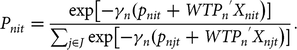 $${P_{nit}} = {{{\rm{exp}}\left[ { - {\gamma _n}({p_{nit}} + WT{{P_n}^{'}}{X_{nit}}} \right)]} \over {\mathop \sum \nolimits_{j \in J} {\rm{exp}}\left[ { - {\gamma _n}({p_{njt}} + WT{{P_n}^{'}}{X_{njt}}} \right)]}}.$$
In equation (3), vector γ n WTP ncan be defined as β n . Using this definition, one can formulate the unconditional probability. This would be the probability that the sequence of choices across choice sets t that individual n made is realized. The probability mass function and cumulative distribution function of the distribution can be specified as follows:
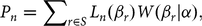 $${P_n} = \sum \nolimits_{r\in S} {L_n}\left( {{\beta _r}} \right)W\left( {{\beta _r}{\rm{|}}\alpha } \right),$$
 $$W\left( {{\beta _r}{\rm{|}}\alpha } \right) = {{\rm{exp}\left[ {\alpha 'z\left( {{\beta _r}} \right)} \right]} \over {\mathop \sum \nolimits_{r \in S} \rm{exp}\left[ {\alpha 'z\left( {{\beta _s}} \right)} \right]}}.$$
For the set of equations (4) and (5), S defines the support set, while z(B r ) captures the distributional shape of the probability mass function. These models allow the distribution to be of any parametric shape (e.g., normal, log normal, etc.). Though parametric distributions accommodate for heterogeneity more than a fixed parameter, they still rely on the idea that the responses will follow a specific distribution. The challenge is that researchers evaluating choice data have to decide which distribution they believe best represents the reactions of subjects. To allow more flexibility and better fit to the WTP coefficients, Train (Reference Train2016) suggests the use of Legendre polynomials. Unlike parametric approaches, polynomials do not make any assumptions about the inherent distribution of the data but instead accommodate the shape of each individual data set.
The analysis presented in this study follows the aforementioned procedure. The five nonprice attributes were estimated as random variables in the WTP space. During the estimation procedure, we used different orders of polynomials to test which fit the data best. The results of a likelihood ratio test showed that a twelfth-order polynomial for the distribution of the WTP coefficients provides the best fit to the data. Therefore, the results of the analysis shown in this study come from the estimation of the parameters using the twelfth-order polynomialsFootnote 1 . The intent of this section is to provide a framework for the results. A complete explanation of the estimation of random parameter models with flexible distributions is outside of the scope of this study. For more details on the process, see Train (Reference Train2016).
3.3. Research hypotheses
To formally present our research questions, we propose the following hypotheses:
Hypothesis 1: Subjects with different levels of attention choose differently. Using the attention level classification from the CRT scores, the sample can be split into two groups: attentive and nonattentive. If subjects are less attentive, then their decision patterns will not be the same as those subjects who are paying attention. These differences in choices will yield different values for the different product attributes when estimating WTP.
Hypothesis 2: Not all attributes evaluated are equally important. The main objective of this study is to be able to provide guidance to breeders of rosebushes on which attributes are important for potential buyers. The selection of attributes for the design of the DCE provides an identification strategy that can help rank the relative importance of the attributes considered.
Hypothesis 3: The WTP for the attributes does not follow a parametric distribution. Assuming a particular statistical distribution ex ante is a common practice in the estimation of choice models with random parameters. If the data do not follow the specified distribution, the model results may not reflect reality. The econometric estimation of this study uses Legendre polynomials to allow for a better fit of the model to the data and to illustrate the difference that would result from the use of a parametric assumption.
Hypothesis 4: The relative importance of different attributes is different for consumers and breeders. A central point in this study is that research priorities in rose breeding are very difficult to establish. Furthermore, it is not certain that the importance of rosebush attributes for breeders has a market. The customer-based approach of this study could not only shed some light on how to direct the research efforts, but also help align the expectations of the market with the aspirations of breeders.
4. Results
A total of 152 subjects participated in the study. Responses from 7 subjects had to be removed from the sample because of data quality issues, such as not having full demographic information, poor eye-tracking calibration, and so forth. Of the remaining 145 subjects, more than 65% self-identified as Caucasian. Nearly two-thirds of the sample was made up of women. The vast majority (more than 95%) of the participants had a college education. The mean reported income of subjects was $64,500 per year.
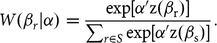
One key result of this study is that attentive and nonattentive subjects behave differently (hypothesis 1). To evaluate this, the CRT scores were used to split the sample into attention groups. Chavez, Palma, and Nayga (Reference Chavez, Palma and Nayga2018b) validated with pupil dilation the use of CRT as an accurate measure of attention. Following the same procedure, subjects who scored a zero on the CRT were categorized as not attentive; everybody else was categorized as an attentive subject as they were to some degree attending to the study. The most striking result that was captured by the classification is that nonattentive subjects comprise half of the sample. This is important because if researchers are to use only the data of attentive subjects for evaluations, the sample sizes would have to be increased. The summary demographics (Table 1) show a pattern of individual characteristics that distinguish attentive from nonattentive subjects in our sample. Attentive subjects tend to be younger. Men and members of racial minorities in the sample are also more likely to be attentive. Attentive subjects have higher numeracy skills (ρ = 0.50).
Table 1. Summary of means of demographics in the sample
Note: Standard errors in parentheses.
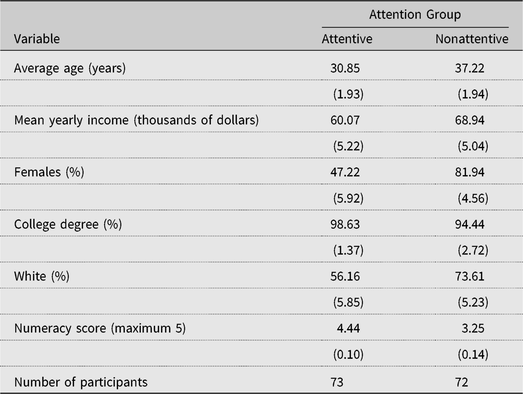
To illustrate how behavior is different for subjects who are attentive compared with those who are not, the data from the eye-tracking device are used. Two visual search metrics in particular exemplify this point. The first metric is the time to first fixation (TFF). TFF is a measure of the time it takes for subjects to look at a particular area on the screen, an area of interest (AOI), once the slide with a stimulus has been presented to them. For this study, the AOIs are the coordinates on the computer screen where the attributes of the choices are located. The second metric used is the total visit duration (TVD). This is a sum of the total time that a subject spends looking at a particular AOI. The summary of these metrics for the two attention groups are in Table 2.
Table 2. Eye-tracking metrics by attention groups
Notes: Standard errors in parentheses. Asterisks (*, **, and ***) denote significance at the 10%, 5%, and 1% level, respectively.
The units of measurement for TFF and TVD are milliseconds (Table 2). In TFF, a lower number means that subjects had faster reaction times to reach an AOI. The results show that for almost all of the attributes presented, the TFF is statistically lower (P < 0.01) for attentive subjects than for nonattentive subjects. Individuals who were attentive reacted faster and focused on the choice task sooner than nonattentive subjects. Attentive subjects also spent more time pondering the choice set as a whole, but for most attributes, the differences are negligible, except for drought and disease tolerance, where attentive subjects spent more time than the nonattentive subjects.
The metrics in Table 2 also shed some light on the relative importance of rose attributes (hypothesis 2). The most visited attributes (TVD) by both attention groups are heat and drought tolerance, followed by foliage coverage, bloom size, price, and, finally, disease tolerance. It is also interesting that though drought tolerance is not the first attribute in the choice sets (see Supplementary Appendix B), both attention groups focused on drought tolerance before any other attribute (i.e., it has the lowest TFF). Similarly, both groups have disease tolerance as the last attribute that caught their attention.
These metrics need to be evaluated carefully though. Some literature suggests that lower visit duration or later visit time may indicate subjects did not tend to the attribute (Orquin and Mueller Loose, Reference Orquin and Loose2013). This approach, however, ignores that subjects may recall information from memory, nor does it account for familiarity with the different attributes. That is to say, the eye-tracking metrics give a starting point for the evaluation of importance of the attributes, but they do not provide a one-to-one correspondence. The econometric estimation provides a complementary measure of relative importance of the rose attributes.
Comparing eye-tracking metrics between attention groups shows that participants exhibit different search behavior. Do these differences in search patterns yield different choices? To evaluate this question, we estimate a random parameters logit model in WTP space. Within the random parameters framework, to account for individual taste heterogeneity the model uses Legendre polynomials for more flexibility and a better fit to the data. Table 3 shows the results of the estimation. Ranking the attributes by marginal WTP reveals that heat and disease tolerance had the highest WTP regardless of the level of attention. The WTP for heat tolerance ranged between $4.26 and $20.00 for attentive subjects, with a mean of $14.51. The mean WTP for heat tolerance among nonattentive subjects was $15.33, with a wider range from –$4.73 to $19.92. Disease tolerance had a mean WTP of $9.94 (ranging from –$19.84 to $19.84) for attentive subjects and a mean of $13.38 (ranging from –$10.86 to $19.84) for nonattentive subjects (Table 3).
Table 3. Random parameter logit estimates with flexible mixing distributions

Notes: Standard errors in parentheses. Asterisks (*, **, and ***) denote significance at the 10%, 5%, and 1% level, respectively. SD, standard deviation.
Drought tolerance, with mean WTP of $9.63 (varying from –$0.34 to $19.84) for attentive subjects and mean WTP of $9.68 (varying from –$9.10 to $19.60) for nonattentive subjects, was the third ranked attribute by WTP. It was followed by bloom size, which for attentive subjects had a mean WTP of $5.85 (varying from –$1.98 to $15.20) and for nonattentive subjects had a mean WTP of $3.62 (varying from –$12.93 to $15.73). Results indicate that foliage coverage was the least important attribute for consumers with mean WTP of $5.12 and a range of –$5.87 to $20.00 for attentive subjects and mean WTP of $1.90 with a range from –$5.41 to $14.68 for nonattentive subjects (Table 3).
A likelihood ratio test revealed that the model estimated pooling the data from attentive and nonattentive subjects was structurally different than models with the data split by attention level (P < 0.01). This indicates that attentive and nonattentive subjects should not be pooled together. This result is supported with the parameter estimates in Table 3. With the exception of heat and drought tolerance, a Haussman test showed that all the parameters were structurally different between the models for attentive and nonattentive subjects. Attentive subjects have a positive WTP for all the attributes. Inattentive subjects are indifferent to foliage coverage but have a positive WTP for all the other attributes.
The effect of attention in the mean WTP can be further illustrated in the distributions of the WTP values. Figures 1–5 show the distributional graphs of WTP for each attribute for attentive (left) and nonattentive subjects (right). A simple eyeball test indicates that the distributions of the WTP are different for subjects who paid attention to the task versus those who did not across all attributes. This result was confirmed using Kolmogorov-Smirnov and Kruskall-Wallis tests, which revealed that the distributions were statistically different (P < 0.001). The distributions of WTP were not normal for any attribute (hypothesis 3). With the exception of the WTP for large blooms for attentive subjects (P > 0.08), Shapiro-Wilk tests showed that the hypothesis that the distributions were normal was rejected (P < 0.001). This result provides support for the use of polynomials in lieu of parametric distributions for the estimation of random parameter choice models.
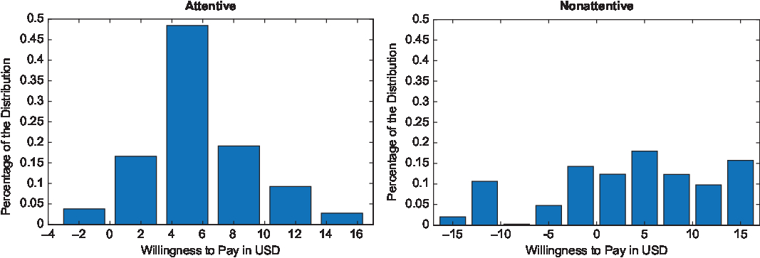
Figure 1. Distributions of willingness to pay (WTP) for large blooms for attentive and nonattentive subjects.
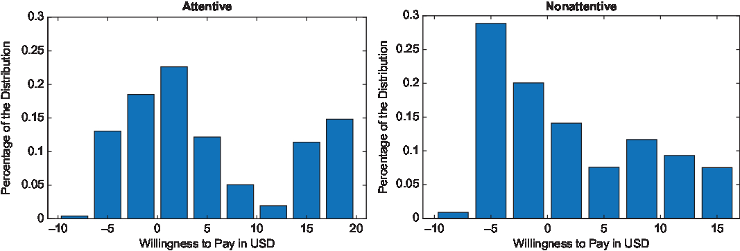
Figure 2. Distributions of willingness to pay (WTP) for high foliage cover for attentive and nonattentive subjects.
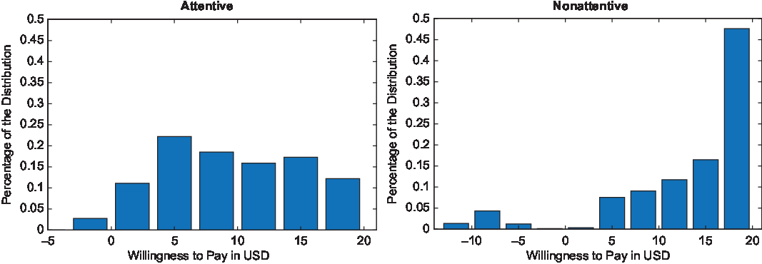
Figure 3. Distributions of willingness to pay (WTP) for disease resistance for attentive and nonattentive subjects.
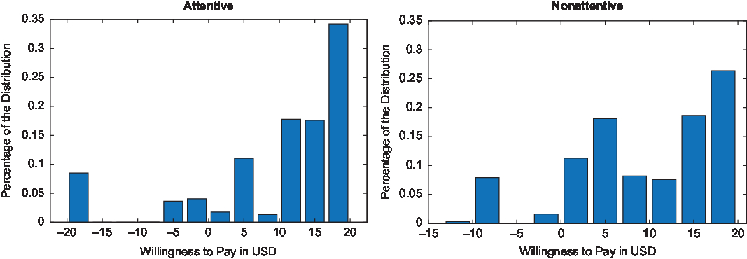
Figure 4. Distributions of willingness to pay (WTP) for drought resistance for attentive and nonattentive subjects.

Figure 5. Distributions of willingness to pay (WTP) for heat tolerance for attentive and nonattentive subjects.
The relative rankings of the different rose attributes by consumers are remarkably informative. As part of the study we conducted a survey of 20 rose breeders. More than half of the breeders surveyed were either in China or the United States. Along with questions about their agricultural practices, distribution channels, and so forth, the survey asked them to evaluate 21 different rose attributes and to rank the importance of the different rose attributes in their breeding efforts. The value of the consumer-based evaluations becomes evident when contrasting them with the breeding effort rankings. The results of the present study align with breeders’ priorities only on disease resistance, which is the most valuable rose attribute for consumers in this study and was regarded as the most important rose attribute by breeders.
Other than that, the two samples provide different rankings. Heat and drought tolerance, which are the more valuable attributes for consumers, are not even in the top 10 priorities for rose attribute breeding. On the other hand, flower size and foliage coverage were ranked sixth and tenth, respectively, by rosebush breeders, while subjects in the present study valued them the least of the rose attributes presented. The results from the consumer side are region dependent, which highlights the importance of conducting more research of this nature for rose breeders in other regions. For example, in the northeastern region of United States, cold hardiness would rank higher, and it would be interesting to see what the consumer preference would be on disease resistance.
What this contrast shows is that rosebush breeders consider the input from consumers in their region to tailor their breeding programs. Without doing so, breeders might be leaving money on the table or applying their resources to developing traits that have little or no influence on consumer demand. It is important to highlight that the present study does not evaluate all the rose attributes considered priorities by rosebush breeders and reinforces the need for additional research to further explore consumer valuations to better inform rosebush breeders.
5. Conclusions
Roses are an important economic commodity in the horticultural sector. The genetic improvement of roses, however, is a long and expensive process. One such challenge is choosing the breeding priorities as some attributes of interest might be mutually exclusive. In an attempt to guide breeders’ priorities, the present study gathered preferences from potential consumers of garden roses. This study used the DCE methodology to identify trade-offs between five different rosebush attributes: heat tolerance, disease resistance, drought tolerance, bloom size, and foliage coverage. The results in this article show that heat and disease tolerance were the most important attributes for consumers in the southern United States. This was indicated by consumers’ higher WTP for these attributes. Ranking the rest of the attributes by WTP, drought tolerance and bloom size were next in relevance. Finally, foliage coverage was the least valuable attribute for consumers. The contrast of the breeders’ priorities and consumer valuations highlights the importance of listening to the voices of customers when establishing breeding programs. More research on consumer valuations of different rose attributes would better inform breeders about where to focus their efforts and resources.
This article also contributes to the literature by using CRT as a means to classify the subjects into attention levels. This classification is important because the choices made by different attention groups differ enough to yield different WTP parameter estimates. The differences in these parameter estimates manifest not only in the means of the estimates, but also in the distributions. This leads to another interesting contribution of this article. The distributions of the parameter estimates are not normal, so the use of polynomials in the estimation helps fit the model better and is a more precise reflection of the actual behavior of consumers. This article provides breeders and geneticists with a market valuation of the attributes used in the design. More research is needed to evaluate different attributes of rosebushes. With the ever-changing landscape of horticultural production and differences in customer preferences dependent on the region, the findings of this study can serve as groundwork for future research.
Financial support
This work was funded by the USDA’s National Institute of Food and Agriculture (NIFA) Specialty Crop Research Initiative project, “Combating Rose Rosette Disease: Short Term and Long Term Approaches” (2014-51181-22644/SCRI).
Supplementary material
To view supplementary material for this article, please visit https://doi.org/10.1017/aae.2019.28


 Open access