


1. Introduction
Surveys have shown that farmers consider access to sufficient capital as one of their biggest hurdles to starting and growing a farm business (Lusher-Shute, Reference Lusher Shute2011). About 5% of U.S. farm sole proprietorships report either being turned down for loans or not applying for credit for fear of denial within the previous 5 years (Briggeman, Towe, and Morehart, Reference Briggeman, Towe and Morehart2009). A larger group of farmers can also be considered credit constrained in the sense that their private demand for credit exceeds the amount that lenders are willing to loan to them (Petrick, Reference Petrick2005). That is, even farmers who can borrow may be effectively constrained because they lack sufficient income or collateral to qualify for a larger loan.
Agricultural lenders ration loans partly based on an assessment of a potential borrower’s ability to repay debt using farm and off-farm income. Commonly used indicators of repayment capacity, such as the “capital debt repayment margin” and the “term-debt and capital-lease coverage ratio,” compare debt payments to available household income (FFSC, 2017). For farm real estate loans, lenders also require substantial collateral. Commercial banks generally do not make loans for farm real estate with loan-to-value ratios greater than 60–70% (U.S. Congressional Oversight Panel, 2009). Although regulations permit Farm Credit System (FCS) loans up to 85% of the value of the real estate, the loan-to-value ratio for FCS loans is typically around 50% (FCSA, 2015).
Individuals who are limited in how much they can borrow by their household income and net worth may be less likely to begin a farm business or to expand an existing operation. Research has found that entrepreneurs tend to be significantly wealthier than those who work in paid employment and that wealthier individuals are more likely to become entrepreneurs (Gentry and Hubbard, Reference Gentry and Hubbard2004). Other research has found that positive exogenous household income shocks, such as from bequests or lottery earnings, are associated with greater levels of small business formation, capital use, and business performance (Blanchflower and Oswald, Reference Blanchflower and Oswald1998; Holtz-Eakin, Joulfaian, and Rosen, Reference Holtz-Eakin, Joulfaian and Rosen.1994; Hurst and Lusardi, Reference Hurst and Lusardi.2004).
Higher off-farm income could relax a farmer’s credit constraint by increasing repayment capacity and the ability to accumulate collateralizable assets (Briggeman, Reference Briggeman2011). Greater access to credit could permit more on-farm investment which, in turn, could raise profits and productivity. Such a connection between off-farm income, credit access, and economic efficiency could provide a justification for government programs that aim to increase access to credit for farmers with limited income and collateralizable wealth.Footnote 1 In this study, we investigate whether there exists such a connection. We estimate the extent to which higher off-farm income leads to more farm-related borrowing and investment in farmland and equipment, and we estimate the relationship between off-farm income and farm labor use, labor and capital input intensity, farm size, farm profits, and productivity.
Off-farm income is an important component of household income for most U.S. farmers. Over 96% of family farms earn some off-farm income and about 86% of the total income of the average farm household originates from off-farm sources (Table 1). For the 95% of family farms with a value of production less than $500,000, over 97% of all household income comes from off-farm sources. Even for the largest 5% of family farms with at least $500,000 in production value, off-farm income represents more than a fifth of total household income. Despite the importance of off-farm income, there is little quantitative information about how it influences farm borrowing and investment, and its role in determining input use, farm size, profits, or productivity.
Table 1. Off-farm income as a share of household income for all family farms, 2007–2016
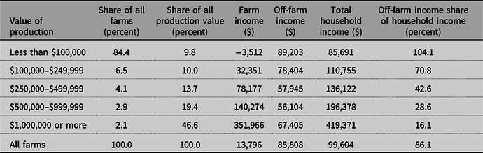
Note: values in 2016 dollars. Farm income includes the household’s share of farm business income, wages paid to household members, farmland rental income, and other farm-related income. Off-farm income includes wages and salaries, net earnings from other businesses, interest and dividends from investments, transfer payments, and other off-farm income.
Source: USDA Agricultural Resource Management Survey, 2007–2016.
This study’s focus on off-farm income is distinct from past research that explored the relationship between off-farm labor supply and farm outcomes. While an exogenous increase in off-farm income should lead, in theory, to greater borrowing and investment given imperfect credit markets, the relationship between the off-farm labor supply and borrowing or investment is ambiguous (Ahituv and Kimhi, Reference Ahituv and Kimhi.2006; Goodwin and Mishra, Reference Goodwin and Mishra2004; Lien, Kumbhaker, and Hardaker, Reference Lien, Kumbhakar and Hardaker2010). This is because an increase in the supply of labor off-farm means there is less household labor available for on-farm work—which, in turn, could limit the desired farm size and the demand for credit. Indeed, Ahituv and Kimhi (Reference Ahituv and Kimhi.2006) analyzed Israeli farm households’ joint off-farm labor and farm capital investment decisions and found a strong negative association between off-farm work and farm capital accumulation. Off-farm labor supply also has a theoretically ambiguous relationship with farm productivity, and this has been reflected in empirical studies. Goodwin and Mishra (Reference Goodwin and Mishra2004) found that greater participation in off-farm labor markets was associated with lower farming efficiency in the U.S. In contrast, Lien, Kumbhaker, and Hardaker (Reference Lien, Kumbhakar and Hardaker2010) found no systematic relationship between off-farm work and farm technical efficiency in Norway.
Past research examining how off-farm income affects farm investment has been limited to developing country contexts (Adams, Reference Adams1991; Rozelle, Taylor, and de Brauw, Reference Rozelle, Taylor and de Brauw1999; Taylor, Rozelle, and de Brauw, Reference Taylor, Rozelle and de Brauw2003). Consistent with the existence of binding credit constraints, most of these studies have found that remittances (off-farm income sent to households by migrants) are associated with increased farm investments. Using data from Mexico, Pfeiffer, Lopez-Feldman and Taylor (Reference Pfeiffer, Lopez-Feldman and Taylor2009) tested whether off-farm income affected agricultural production activities, technologies, and input use by comparing households that received remittances with similar households that did not. The authors found that remittances had a negative effect on agricultural output and the use of family labor on the farm, but a positive impact on the demand for purchased inputs and on farm efficiency.
A challenge with estimating the effect of off-farm income on borrowing and investment is the fact that the household’s labor allocation decision—and hence its off-farm income—is simultaneously determined with other farm decisions. Individuals with higher off-farm income generally work more hours off the farm and fewer hours on the farm. Hence, households with higher off-farm income tend to have smaller operations and, consequently, less demand for farm inputs and investment. As shown later in the paper, this can result in a non-causal negative correlation between off-farm income and investment.
Past studies have attempted to identify exogenous variation in off-farm income by using instruments that affect the off-farm wage or the incentive to work off-farm, such as the distance to an international border or measures of local economic conditions. However, it is not clear that these instruments affect the outcome variables exclusively through their effect on off-farm income (a necessary condition for a valid instrument). For example, farms located closer to an international border will have more family members who migrate, and will earn more off-farm income, on average. But farm households with more migrants will have less household labor available to work on the farm. In the presence of labor market imperfections, these households will generally have smaller farms that require less on-farm investment. In sum, the instrument affects investment partly through the labor use decision, which can cause a spurious inverse correlation between off-farm income and investment.
In this study, we use the educational attainment of the operator’s spouse to identify an exogenous source of variation in off-farm income: spouses with more education will tend to earn higher off-farm wages. A potential endogeneity issue arises because better-educated spouses earn higher wages and therefore tend to work more hours off-farm (Gould and Soupe, Reference Gould and Soupe1989; Huffman, Reference Huffman1980. Huffman and Lange, Reference Huffman and Lange1989). This causes education to be correlated with farm labor use and, consequently, other farm-related decisions. We sever the link between the off-farm wage rate and farm labor use by only considering households where the spouse does not work on the farm. For these farms, variation in the spouse’s educational attainment should affect the spouse’s off-farm wage, but should not, as we show in the paper, directly affect on-farm labor use or borrowing, investment, or other farm-related decisions. This allows for a plausible assertion that the link between off-farm income and farm borrowing and investment is causal.
While spouses with higher education might have the greater farming ability, this should also have no direct effect on farm outcomes because the spouses in the sample do not spend any time working on-farm. Of course, it is possible that the spouse’s educational attainment is positively, though imperfectly, correlated with the operator’s educational attainment—people with similar attributes might be more likely to marry each other. This could result in a correlation between the spouse’s off-farm income (which is partially determined by the spouse’s education level) and farm borrowing and other farm outcomes (to the extent that they are determined by the operator’s education). We address this possibility by directly controlling for the operator’s educational attainment in the outcome regressions. This allows us to estimate the effect of a change in off-farm income holding the operator’s education constant.
As far as we are aware, this is the first study to estimate the effect of an exogenous change in off-farm income on borrowing, investment, and productivity for U.S. farms. We find that greater off-farm income leads to higher levels of farm borrowing and capital expenditures, and that the marginal effect is largest for young–beginning farmers. Results indicate that higher household income (from the spouse’s off-farm income) causes principal operators to increase their time spent working on-farm and to reduce their time spent working off-farm. We also find that more off-farm income leads to an expansion in farm size (measured in terms of production value and assets) and to a more capital-intensive input mix (labor value declines and interest costs increase as a share of total expenses). Finally, we find evidence that higher off-farm income increases farm profits and productivity. The results are consistent with the existence of credit rationing and suggest that government programs to increase access to loans for credit-rationed farmers could enhance economic efficiency in the agricultural sector.
2. Empirical Approach
We use the educational attainment of the farm operator’s spouse as an instrument to identify exogenous variation in off-farm income. A valid instrument should be strongly correlated with the explanatory variable of interest (off-farm income) but not be correlated with unobservables affecting the outcome variables (farm decisions such as borrowing and capital expenditures). With imperfect markets, a spouse’s education could potentially be correlated with unobservables affecting farm business decisions if a spouse were involved with the farm work. For example, a spouse with more education might earn more and thus work less on-farm, or might make better farm management decisions, resulting in higher output. However, as we show below, among the subset of farms where the operator’s spouse does not work on the farm, the spouse’s education should have no indirect effect on farm production decisions. That is, the spouse’s education should only affect the outcome variables through off-farm income.
In the standard perfect markets farm household model, household members allocate their time between farm and off-farm work to maximize utility, which means they equate the marginal value of time each activity (Sumner, Reference Sumner1982). When the separate decisions of the farm operator and spouse are modeled in the standard model, it can be shown that the off-farm labor supply of the operator (spouse) depends on whether and how much the spouse (operator) works off-farm (Huffman and Lange, Reference Huffman and Lange1989). However, with perfect markets, the labor allocation decisions of the operator and spouse do not directly affect production—household labor is a perfect substitute for hired labor and labor of either kind is applied on-farm until the marginal value product of labor equals the market wage. Hence, with perfect markets, changes in off-farm income will not alter production decisions. If a spouse earns a higher wage because of higher educational attainment, then the spouse supplies more labor off-farm and less on-farm, but total on-farm labor and production do not change.
If credit markets are imperfect then the household’s consumption and production decisions become non-separable (Briggeman, Towe, and Morehart, Reference Briggeman, Towe and Morehart2009; De Janvry et al., Reference De Janvry, Sadoulet, Fafchamps and Raki1992; Karlan et al., Reference Karlan, Osei, Osei-Akoto and Udry2014; Petrick, Reference Petrick2005; Pfeiffer et al., Reference Pfeiffer, Lopez-Feldman and Taylor2009). Non-separability implies that factors affecting labor allocation decisions and off-farm income can also affect production decisions. To illustrate, consider a two-period optimization problem for a unitary farm household facing a credit constraint:
 $${\rm{Max }}U( {{C_1},{C_2}} )\,{\rm{w}}{\rm{.r}}{\rm{.t}}{\rm{. }}{C_1},{C_2},{\rm{}}L_o^f,L_s^f,X,K$$
s.t.
 $${w_o}L_o^n + {w_s}( E )L_s^n + I - {p_x}X - {p_c}{C_1} + K = 0$$
 $${p_q}Q \left( {L_o^f,L_s^f,X} \right) - {p_c}{C_2} - ( {1 + r} )K = 0$$
 $$L_o^n + L_o^f = {L_o}$$
 $$L_s^n + L_s^f = {L_s}$$
 $$K \le \overline {K}$$
The household chooses consumption in both periods, ${C_1}$
and
${C_1}$
and ${C_2}$
, operator and spouse farm labor,
${C_2}$
, operator and spouse farm labor, $\;L_o^f$
and
$\;L_o^f$
and $\;L_s^f$
, other farm inputs
$\;L_s^f$
, other farm inputs $X$
(which includes hired labor) and credit
$X$
(which includes hired labor) and credit $K$
to maximize utility subject to budget constraints in each period. To simplify the model, the operator and spouse are assumed to allocate their time endowments,
$K$
to maximize utility subject to budget constraints in each period. To simplify the model, the operator and spouse are assumed to allocate their time endowments, ${L_o}$
and
${L_o}$
and ${L_s}$
, between farm work and non-farm work (indicated with the superscripts f and n, respectively) (equations [4] and [5]). The spouse’s wage rate is a function of the spouse’s educational attainment
${L_s}$
, between farm work and non-farm work (indicated with the superscripts f and n, respectively) (equations [4] and [5]). The spouse’s wage rate is a function of the spouse’s educational attainment $E$
. In the first period (equation 2), the household uses non-farm wage income earned by the farm operator and spouse and other non-farm income
$E$
. In the first period (equation 2), the household uses non-farm wage income earned by the farm operator and spouse and other non-farm income $I$
and credit to purchase consumption goods and farm inputs. In the second period (equation 3), revenues from farm production
$I$
and credit to purchase consumption goods and farm inputs. In the second period (equation 3), revenues from farm production $Q$
are used to purchase consumption goods and to pay back the debt with interest
$Q$
are used to purchase consumption goods and to pay back the debt with interest $r$
. Credit is constrained to be below some maximum
$r$
. Credit is constrained to be below some maximum $\overline K$
(equation 6).
$\overline K$
(equation 6).
As the studies cited in the previous paragraph have shown, at the optimum when the constraint is binding, the marginal profit from purchased inputs equals the input price times the shadow value of liquidity. This means the effective input cost is greater than the market price. Hence, households with a binding credit constraint will purchase fewer inputs than they would otherwise. A similar logic applies to on-farm labor. With a binding credit constraint, the effective wage exceeds the market wage, so a credit-constrained household will use less labor on the farm. The household will either hire less labor or work more off-farm, depending on the demand for farm labor relative to the household’s labor supply (Sadoulet and de Janvry, Reference Sadoulet and de Janvry1995). It follows that if the credit limit $\overline K$
increases (perhaps because an exogenous increase in off-farm income causes a bank to offer more money to the farmer), then the shadow value of liquidity will decrease, resulting an increase in purchased inputs and on-farm labor—and hence an increase in farm output.
$\overline K$
increases (perhaps because an exogenous increase in off-farm income causes a bank to offer more money to the farmer), then the shadow value of liquidity will decrease, resulting an increase in purchased inputs and on-farm labor—and hence an increase in farm output.
A change in off-farm income could also affect the input mix when the credit constraint is binding. Long-term credit for capital equipment or land is more likely to be rationed based on household income and net worth than is short-term production credit, which is often secured by the expected value of the harvest. Hence, an exogenous increase in off-farm income could be expected to relax a long-term credit constraint more than a short-term credit constraint. This would cause the relative shadow price of inputs (machinery and land) purchased with long-term credit to decline more. Hence, an exogenous increase in income may be associated with an increase in the expenditure share of inputs purchased with long-term credit.
To empirically identify the effect of an exogenous increase in off-farm income on farm decisions, we consider only those households in which the spouse works off the farm but not on the farm (the operator may work both on and off the farm). If the spouse does not work on-farm then $L_o^n = {L_s}$
, and the optimization can be simplified to:
$L_o^n = {L_s}$
, and the optimization can be simplified to:
 $${\rm{Max }}U\left( {{C_1},{C_2}} \right)\,{\rm{w}}{\rm{.r}}{\rm{.t}}{\rm{.}}\,{C_1},{C_2},{\rm{}}L_o^f,X,K$$
s.t.
 $${w_o}L_o^n + OF{I_s} + I - {p_x}X - {p_c}{C_1} + K = 0$$
 $${p_q}Q\left( {L_o^f,X} \right) - {p_c}{C_2} - \left( {1 + r} \right)K = 0$$
 $$L_o^n + L_o^f = {L_o}$$
 $$K \le \overline K$$
where the spouse’s off-farm income is defined as the wage times the spouse’s labor endowment: $OF{I_s} = {w_s}\left( E \right)L_s$
. Alternatively, we can expand the definition of the spouse’s off-farm income to include all other non-farm income:
$OF{I_s} = {w_s}\left( E \right)L_s$
. Alternatively, we can expand the definition of the spouse’s off-farm income to include all other non-farm income: $OF{I_s} = {w_s}\left( E \right)L_s$
+
$OF{I_s} = {w_s}\left( E \right)L_s$
+ $\;I$
. We use the second definition of off-farm income in the analysis because it has a positive value for almost all the farms in the sample. But we obtain very similar results when we use the first definition, as we show in the results section. The spouse’s off-farm income is a function of exogenous characteristics and can be expressed generally as
$\;I$
. We use the second definition of off-farm income in the analysis because it has a positive value for almost all the farms in the sample. But we obtain very similar results when we use the first definition, as we show in the results section. The spouse’s off-farm income is a function of exogenous characteristics and can be expressed generally as $OF{I_s}\left( {E,\;L_s,\;I} \right)$
. In linear reduced form, it can be written:
$OF{I_s}\left( {E,\;L_s,\;I} \right)$
. In linear reduced form, it can be written:
 $$OF{I_{si}} = {\alpha _1} + {\beta _E}{E_i} + {\beta _1}{Z_1}_i + {v_i}$$
where the vector ${Z_1}$
includes factors besides the spouse’s education that affect the spouse’s off-farm wage (e.g., local economic conditions), the spouse’s labor endowment (e.g., age), and other non-farm income.
${Z_1}$
includes factors besides the spouse’s education that affect the spouse’s off-farm wage (e.g., local economic conditions), the spouse’s labor endowment (e.g., age), and other non-farm income.
The optimal input and operator on-farm labor levels, $X\left( {OF{I_s},\;{Z_2}} \right)$
and
$X\left( {OF{I_s},\;{Z_2}} \right)$
and $L_o^f\left( {OF{I_s},{Z_2}} \right)$
, can be expressed as functions of the spouse’s off-farm income and other exogenous factors
$L_o^f\left( {OF{I_s},{Z_2}} \right)$
, can be expressed as functions of the spouse’s off-farm income and other exogenous factors ${Z_2}$
affecting preferences, prices, the production technology, and the credit constraint. We are interested in how an exogenous change in off-farm income affects inputs (farm-related borrowing and capital investment) and labor inputs (operator’s labor and total labor). We are also interested in how off-farm income affects input mix, and farm size (output), profits, and productivity. These outcomes
${Z_2}$
affecting preferences, prices, the production technology, and the credit constraint. We are interested in how an exogenous change in off-farm income affects inputs (farm-related borrowing and capital investment) and labor inputs (operator’s labor and total labor). We are also interested in how off-farm income affects input mix, and farm size (output), profits, and productivity. These outcomes ${Y_i}\;$
can be written as functions of the input equations. Hence, in linear reduced form the outcome equations can be written:
${Y_i}\;$
can be written as functions of the input equations. Hence, in linear reduced form the outcome equations can be written:
 $${Y_i} = {\alpha _2} + \theta OF{I_{si}} + {\gamma _2}{Z_2}_i + {u_i}$$
Importantly, a change in the spouse’s education will directly affect the spouse’s off-farm income (equation 7), but this change in income will not affect the amount of time the spouse works on-farm—because the spouse does not work on the farm in the sample. Consequently, there is no independent effect of a change in the education on production decisions (equation 8). Hence, we can use the spouse’s education as an instrument for the spouse’s off-farm income. Of course, education may affect production through off-farm income: greater educational attainment leads to higher off-farm income, which relaxes the budget constraint.
We estimate equations (7) and (8) using a two-stage least squares instrumental variables (IV) model. For some outcomes—including interest expenses, capital expenditures, and non-current liabilities—a large share of the sample reports a zero value. For these outcomes, we use a Tobit model with a continuous endogenous regressor. In this IV-Tobit model, the outcome in equation (8) is a latent variable $Y_i^*$
. We do not observe
$Y_i^*$
. We do not observe $Y_i^*$
; instead, we observe
$Y_i^*$
; instead, we observe ${Y_i} = max\left( {0,Y_i^*} \right)$
. The IV-Tobit model is estimated using a maximum likelihood estimator.Footnote
2
${Y_i} = max\left( {0,Y_i^*} \right)$
. The IV-Tobit model is estimated using a maximum likelihood estimator.Footnote
2
3. Data
A sample of farm households is assembled using data from 10 years (2007–2016) of the Agricultural Resource Management Survey (ARMS). The ARMS is an annual U.S. Department of Agriculture (USDA) survey carried out by the National Agricultural Statistics Service and Economic Research Service (ERS). It is the USDA’s primary source of information about farm income and farm household finances.
Exogenous variables thought to influence borrowing and farm production decisions include the operator’s age, education, and sex (the spouse’s age is not observed and the spouse’s sex almost perfectly predicts the operator’s sex so is not included in the econometric model). As discussed in the “Introduction” section, we include the operator’s education in the regression to address the possibility of a spurious correlation between the spouse’s off-farm income and farm outcomes that might result because of a correlation in the educational levels of the spouses and operators.
Other variables thought to affect farm decisions include indicators of commodity specialization (19 categories) and state indicators meant to capture intrinsic differences across states in farm profitability that are due to climate, soil differences, etc. We also include a year indictor, to capture annual variation in commodity and input prices and interest rates.
Outcome variables fall into several categories, including: (1) borrowing (total farm business debt, current and non-current liabilities, and interest expenses); (2) investment (current period farm-related capital expenditures, which includes spending on improvements, construction, trucks, tractors, machinery, and real estate); (3) labor use (a value of all labor used on-farm, the operator’s on-farm labor hours, and the operator’s off-farm income; (4) farm size (a value of production and total farm assets); (5) income (farm income to the household and net farm income); (6) net worth; and (7) productivity (gross cash farm income divided by total expenses).
To measure the operator’s off-farm labor supply, we use the operator’s off-farm income instead of off-farm labor hours because a question about the operator’s off-farm labor hours was not included in the ARMS in several years of the survey between 2007 and 2016. “Farm income to household” includes the household’s share of farm business income, wages paid to household members, farmland rental income, and other farm-related income. “Net farm income” is gross farm income (gross cash farm income plus the change in the value of inventory plus the rental value of farm dwelling) minus cash expenses including depreciation. All monetary values are inflated to 2016 values using the Bureau of Economic Analysis (BEA) implicit price deflator.
Means for the key variables used in the study are shown in Table 2 for all family farms, family farms with a married operator, and family farms with a married operator whose spouse does not work on the farm. About 80% of all family farm operators report having a spouse. In 44% of these households the spouse does not work on the farm, so this group comprises about 35% of all family farms. Table 2 shows that family farms on which the spouse does not work on the farm (column 3) have characteristics that are very similar to the entire family farm population (column 1) and to the sample in which the operator is married (column 2).
Table 2. Comparison of key variables for family farms depending on operator’s marital status and spouse’s work status
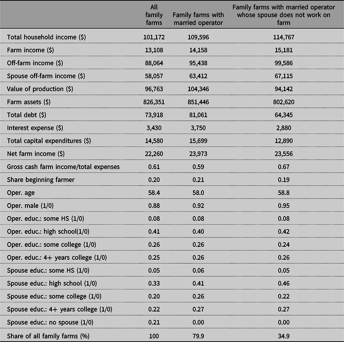
Note: values in 2016 dollars. Spouse’s off-farm income includes non-farm income to the household. “Total expense” is the cost of all inputs to production including the estimated opportunity cost of unpaid labor used on-farm. Gross cash farm income (GCFI) is annual income before expenses and includes commodity cash receipts, farm-related income, and government farm program payments. “Net farm income” is gross farm income (GCFI plus change in value of inventory plus rental value of farm dwelling) minus cash expenses including depreciation.
Source: USDA Agricultural Resource Management Survey, 2007–2016.
4. Results
Table 3 previews some of the main results of the IV regressions using a simple comparison of means. Farm households are categorized in two ways: by off-farm income quartiles (top half of table) and by the spouse’s education (bottom half of table). The first two columns in the top half of the table show that higher off-farm income is associated with lower farm income. For example, farms in the bottom off-farm income quartile earn $25,298 in farm income compared to only $6,782 for those in the top off-farm income quartile. This negative relationship is likely partly explained by the fact that in households with higher off-farm income the operator spends more time working off-farm and less time working on-farm. Households with smaller operations, where the operator spends less time working on-farm, will generally invest less in the farm. This is confirmed by the last three columns in the table, which shows the negative relationship between off-farm income and borrowing and investment. For example, the average households in the bottom off-farm income quartile had $73,945 in total farm debt, compared to $58,297 for households in the top quartile.
Table 3. Income, borrowing, and capital expenditures by off-farm income quartile and spouse’s education: farms where spouse does not work on-farm
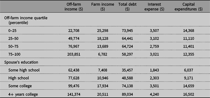
Note: values in 2016 dollars. Total debt includes all farm-related current and non-current liabilities (loan balances, accrued interest, and accounts payable).
Source: USDA Agricultural Resource Management Survey, 2007–2016. The sample includes family farms where the operator’s spouse does not work on-farm.
The bottom half of Table 3 shows the relationship between the spouse’s education and the outcome variables. As would be expected, off-farm income increases with the spouse’s education. In the sample, spouses do not work on-farm, so higher off-farm income resulting from higher spouse education does not imply less time spent on the farm. In fact, farm income increases with the spouse’s education as does borrowing and investment. For example, farm-related debt for households where the spouse does not have a high school degree averaged only $35,457, compared to $89,034 for households where the spouse has at least 4 years of college education. As shown in the next section, the positive relationship between the spouse’s education and the measures of farm income, borrowing, and investment is reflected in the results of the IV regressions, which use the spouse’s education as an instrument for off-farm income.
4.1. IV Regressions
A separate first-stage regression (Table 4) shows that greater educational attainment results in higher off-farm income for the spouse: compared to spouses who did not complete high school, spouses with a high school diploma earned 33% more off-farm income, spouses with less than 4 years of college earned 46% more, and spouses with a 4 year college degree earned 79% more.
Table 4. First-stage regression: log of spouse’s off-farm income
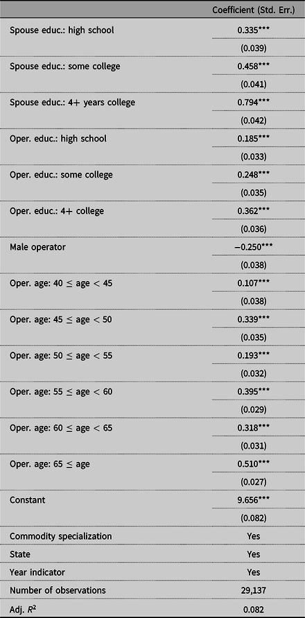
Note: standard errors in parentheses. ***P < 0.01, **P < 0.05, *P < 0.1.
Source: USDA Agricultural Resource Management Survey, 2007–2016. The sample includes family farms where the operator’s spouse does not work on-farm.
The first-stage F statistic and Wald statistic provide tests of weak identification and underidentification, respectively (Angrist and Pischke, Reference Angrist and Pischke.2009). Weak identification arises when the excluded instruments are weakly correlated with the endogenous regressors, which may cause the estimator to perform poorly (Stock and Yogo, Reference Stock, Yogo, Andrews and Stock2005). The first-stage F statistic can be compared to the Stock and Yogo (Reference Stock, Yogo, Andrews and Stock2005) critical values for the Cragg–Donald F statistic. In our case, the F statistic has a value of 218, which is well above the Stock–Yogo critical values (which range between 5 and 22 based on test assumptions) indicating that the endogenous regressor is not weakly identified.
The Angrist–Pischke underidentification test is a test of whether the excluded instruments are “relevant”—that is, correlated with the endogenous regressors. The Angrist–Pischke Wald statistic is distributed as chi-squared under the null that the endogenous regressor is unidentified. In our case, the test statistic has a value of 649 with a P value of <0.0001, indicating that the model is not underidentified.
We also evaluate the validity of the instruments by testing whether the excluded instruments are appropriately independent of the error process. We perform a test of overidentifying restrictions by regressing the residuals from the IV regression on all the instruments. Under the null hypothesis that the instruments are uncorrelated with the error in the outcome equation, the test has a chi-squared distribution and under the assumption of i.i.d. errors is known as a Sargan test. In our case, for the five outcome equations (Table 5) the Sargan test statistic has a P value ranging from 0.72 to 0.96. Hence, we cannot reject the null hypothesis that the overidentifying restrictions are valid.
Table 5. Second-stage IV regressions: borrowing and investment
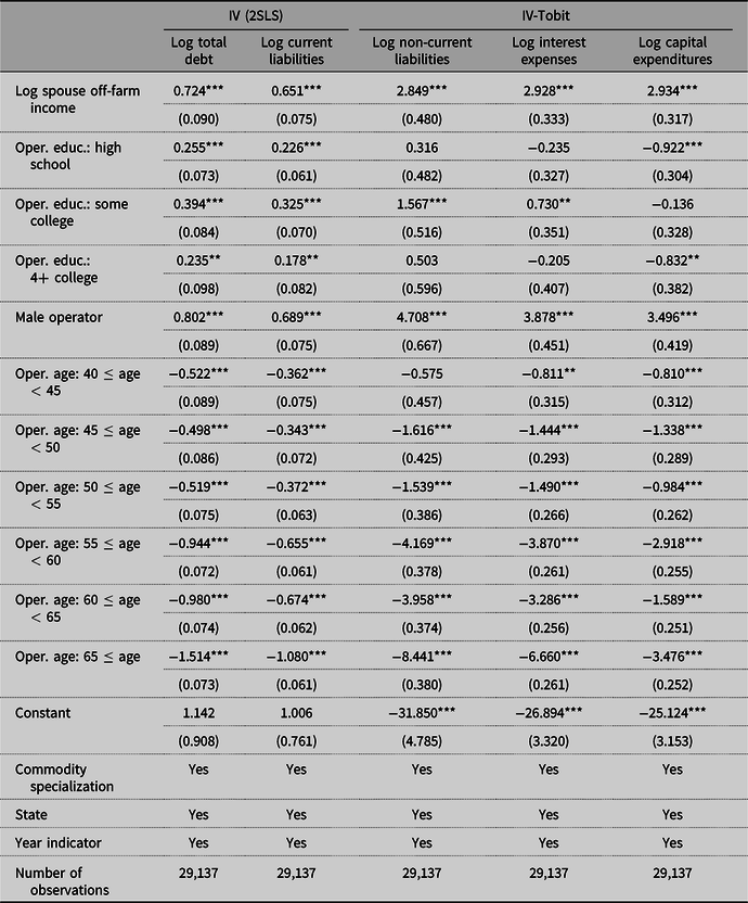
Note: standard errors in parentheses. ***P < 0.01, **P < 0.05, *P < 0.1.
Source: USDA Agricultural Resource Management Survey, 2007–2016. The sample includes family farms where the operator’s spouse does not work on-farm.
The second-stage IV estimates show that off-farm income increases borrowing and investment (Table 5). Because of the highly skewed nature of the income and debt variables, we use logarithms to reduce the effect of extreme values on the outcomes. Results indicate that a 1% increase in the spouse’s off-farm income is associated with increases of 0.7% for total debt, 0.6% for current debt, 2.9% for non-current debt, 3.0% for interest expenses, and 3.0% for capital expenditures.Footnote 3 The effect on non-current debt and capital expenditures is substantially larger than the effect on current debt (and on total debt, which is dominated for many farms by current debt, because over half of all farms have no non-current debt). This implies that off-farm income allows for a larger increase in long-term capital and land purchases funded by long-term debt. Long-term debt is more likely to be subject to household income and collateral requirements compared to short-term debt. Short-term debt, which can include production loans for seeds, pesticides, and other inputs are often secured by the expected value of the harvest, which makes off-farm income less important (OCC, 2017).
The large and positive effect of off-farm income on borrowing and investment implied by the IV estimates can be contrasted with the much smaller or negative effects implied by naïve ordinary least squares (OLS)/Tobit estimates (appendix Table A1). The OLS/Tobit coefficients imply that a 1% increase in off-farm income is associated with changes in the measures of borrowing ranging between about −0.1% and 0.1%. These results are consistent with the weak negative association between off-farm income and borrowing and investment that was observed in the top half of Table 3.
Table 5 also provides information about how other factors influence farm borrowing and investment. As would be expected, borrowing and capital expenditures tend to decline with age, with a particularly steep drop off in investment for operators over age 65. Male operators tend to invest more than their female counterparts. Greater educational attainment by the operator was generally associated with more borrowing and investment. However, there was little significant difference in the effect of educational attainment beyond the “some college” level.
The appendix Table A2 illustrates that the results are robust to different specifications of the second-stage model using the log of total debt as the dependent variable. The parameter associated with off-farm income is stable across the four specifications (column 4 is the preferred model).
Appendix Table A3 illustrates that the second-stage estimates are also robust to an alternative definition of the spouse’s off-farm income. As discussed above, the spouse’s off-farm income could be defined as wage income alone or wage income plus other non-farm income to the household. Table A3 shows the results of the IV regressions with the spouse’s income limited to wage income. To obtain variation in the instrument across all observations, the sample is limited to households where the spouse earns a positive wage income, which reduces the sample size from 29,137 to 17,437. Nonetheless, the estimated parameters in Table A3 are very similar to those in Table 5. For example, for the logarithm of total debt, the estimated parameter is 0.724 using the more expansive definition of off-farm income, and 0.702 using the more restrictive definition.
Table 6 presents the coefficients associated with the spouse’s off-farm income in the second-stage IV regressions for 11 additional outcome variables using the full model and the more expansive definition of spouse’s off-farm labor. The first three outcomes measure labor use on and off the farm. The results indicate that an exogenous increase in off-farm income leads to an increase in both total and operator labor use on-farm and a decrease in operator off-farm income. This implies that some operators respond to additional off-farm income by shifting from off-farm work to farm work. This is consistent with a binding credit constraint as discussed above. In contrast, for farm households not facing a binding credit constraint, the standard household model implies operators would respond to an exogenous increase in non-farm income by working less off-farm and less on-farm, as the additional income would allow them to “consume” additional leisure.
Table 6. Effect of off-farm income on operator labor, input mix, farm size, farm income, and productivity
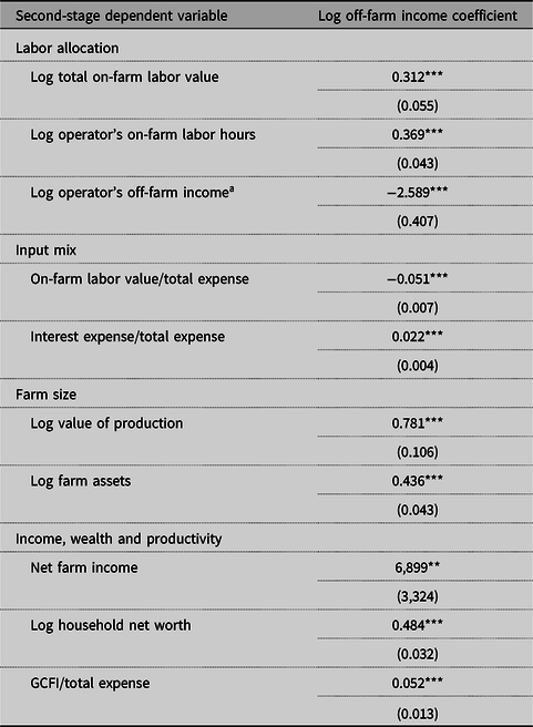
a IV-Tobit estimation.
Note: standard errors in parentheses. ***P < 0.01, **P < 0.05, *P < 0.1.
Source: USDA Agricultural Resource Management Survey, 2007–2016. The sample includes family farms where the operator’s spouse does not work on-farm.
The fourth and fifth variables in Table 6 measure the input mix. Labor intensity is measured as the value of total on-farm labor-to-total expense ratio, where on-farm labor includes the implicit cost of operator labor plus hired labor costs. Capital intensity is measured as the interest expense-to-total expense ratio. The IV regression results indicate that a 1% increase in off-farm income causes a 0.05 percentage point decline in the labor ratio and a 0.02 percentage point increase in the capital ratio. Hence, the results are consistent with off-farm income relieving a long-run credit constraint and shifting the input mix toward a more capital-intensive mode of production.
The six and seventh variables are measures of farm size. The previous results showed that more off-farm labor leads to an increase in borrowing, capital investment, and on-farm labor use. Greater borrowing and input use would be expected to result in more production and a larger farm size. This is confirmed by the IV results which show that a 1% increase in off-farm income increases the total value of farm production by 0.8% and the total value of farm assets by 0.4%.
The last group of outcome variables in Table 6 includes measures of farm income, productivity, and net worth. If a farm faces a binding credit constraint, then a relaxation of the constraint would be expected to result in a more efficient allocation of resources and thus to higher farm profits. This prediction is consistent with the results, which indicate that a 1% increase in off-farm income is associated with a $59 increase in farm income to the household and a $69 dollar increase in net farm income.Footnote 4 These effects can be compared to the average farm household income and net farm income values of $16,067 and $25,091, respectively, for family farms with a married operator whose spouse does not work on the farm (Table 3). This implies increases of 0.4% and 0.3% for farm income to the household and net farm income, respectively.
The results also indicate that an increase in off-farm income leads to an increase in productivity—which is measured using the ratio of gross cash farm income to total expenses. Specifically, we find that a 1% increase in the spouse’s off-farm income is associated with a 0.05 percentage point increase in the productivity index. With an average value of 0.69, this implies an increase of 0.07%. Hence, a 10% increase in the spouse’s off-farm income (an increase of about $6,711) would increase farm productivity by about 0.7%.
The productivity index used in this study does not provide information about the source of productivity differences across farms. Higher productivity could result because the additional borrowing allows farms to use a more efficient (and capital-intensive) product mix. Another not mutually exclusive possibility is that the additional borrowing allows farms to expand to a larger and more efficient scale (Key, Reference Key2019).
Net worth is the last outcome variable shown in Table 6. A household’s net worth will depend on its inherited wealth plus accumulated savings. Households with higher income should be able to save more. Since higher off-farm income was shown to lead to higher farm income, it could be expected that higher off-farm income would be associated with higher net worth. Indeed, the results also indicate that a 1% increase in off-farm income results in a 0.5% increase in net worth.
4.2. Effects by Operator and Farm Subgroups
It is likely that different types of operators and different types of farms will respond in different ways to a change in off-farm income. Farmers likely vary in their access to credit and have different objectives in terms of farm growth depending on their financial positions and on lifecycle factors. In this section, we test how the effects of off-farm income on farm decisions vary by the age and experience of the principal operator (Table 7) and by the size of the operation (Table 8).
Table 7. Effect of off-farm income on borrowing, farm size, profits, and productivity by operator age, and experience
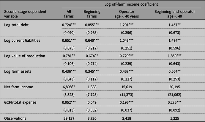
Note: standard errors in parentheses. ***P < 0.01, **P < 0.05, *P < 0.1. A beginning farm has a principal operator with less than 10 years of farming experience.
Source: USDA Agricultural Resource Management Survey, 2007–2016. The sample includes family farms where the operator’s spouse does not work on-farm.
Table 8. Effect of off-farm income on borrowing, farm size, profits, and productivity by farm size
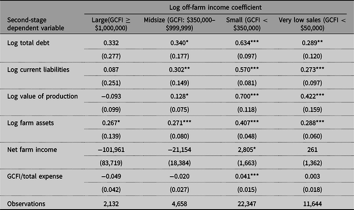
Note: standard errors in parentheses. ***P < 0.01, **P < 0.05, *P < 0.1. GCFI is annual income before expenses and includes commodity cash receipts, farm-related income, and government farm program payments.
Source: USDA Agricultural Resource Management Survey, 2007–2016. The sample includes family farms where the operator’s spouse does not work on-farm.
Farms are classified as “beginning” if the principal operator has no more than 10 years of farming experience and are classified as “young” if the principal operator is less than 40 years old. As discussed above, the second-stage regression results show that borrowing and investment tend to decline with the age of the operator—with the highest levels found among the farms with operators less than 40 years old. Younger and less-experienced farmers may have a high demand for credit, but at that same time may not have the savings or farm income with which to secure sufficient capital. Hence, younger and less-experienced farmers may be more credit constrained, and off-farm income may have a bigger effect on their farm decisions. That is, additional off-farm income may lead to a bigger increase in borrowing for young and beginning farmers, leading to a bigger increase in farm size, income, and productivity. To test this hypothesis, we estimate the effect of off-farm income on seven key outcome variables.
In general, the effects of off-farm income on the outcome variables are not greater for beginning farms compared to all farms (Table 7). In contrast, six out of the seven variables coefficients are larger for young farms (operator less than 40 years old) compared to all farms. Four of these differences are statistically significantly different from zero at the 90% level. For young–beginning farms the marginal effects are even larger: all seven coefficients are larger for young–beginning farms compared to all farms and four of these differences are statistically significant. As an example, a 1% exogenous increase in off-farm income increases total debt by 0.7% for all farms, 0.85% for beginning farms, 1.2% for young farms, and 1.5% for young–beginning farms. For total debt, current liabilities, the value of production, farm income, and productivity, the effects of an increase in off-farm income are statistically significantly larger when the principal operator is both young and beginning.
Next, we explore how the effect of off-farm income on borrowing and other farm decisions varies with the size of the operation. There are several reasons why the effects could vary with farm size. The first stems from the fact that off-farm income represents a diminishing share of total household income as farm size increases. For large operations, a change in the spouse’s income will have a relatively small effect on total household income and therefore should have a proportionately smaller effect on farm-related borrowing. Indeed, Briggeman (Reference Briggeman2011) found that large farms consistently had a farm debt repayment capacity utilization ratio below 100%, implying that operators of these farms could meet their farm debt obligations with farm income alone. This was not the case for operators of small farms, who could not meet their debt obligations without off-farm income.
Another reason why the effect of off-farm income could vary by scale stems from differences in motivations for farming. It has been hypothesized that operators of very small “lifestyle” or “hobby” farms might be less motivated by economic returns and instead place more value on the non-pecuniary benefits from farming than operators of larger commercial operations (Howley, Reference Howley2015; Key and Roberts, Reference Key and Roberts2009). Indeed, a large share of small-scale operations reports negative farm income ever year (Key, Reference Key2019). One possible explanation for why these farmers continue in business despite economic losses is that they derive pleasure from the attributes of farm work. These producers may enjoy the autonomy and independence of farming, the sense of responsibility and pride associated with business ownership, or other social or lifestyle attributes of farming (Howley, Reference Howley2015; Key and Roberts, Reference Key and Roberts2009). Key and Roberts found that, on average, farm households reported earning more per hour off-farm than they did on-farm, and this wage differential was larger for smaller farms. The wage differential implies large non-pecuniary benefits to farming—particularly for very small farms. In addition, the U.S. tax code allows households to use reported farm losses to offset non-farm income and thereby lower total income taxes (Durst, Reference Durst2009). It is possible that operators of small-scale farms, who are motivated by farming’s non-pecuniary or tax benefits, place less emphasis on the economic returns of their farms and are therefore less inclined to invest in their operations in order to increase the scale of production or raise productivity. These farmers may be less likely to borrow for their business in response to an increase in non-farm income.
To assess how the effects vary with scale, we follow the most recent USDA-ERS farm typology (Hoppe and MacDonald, 2013) and divide the sample of family farms into three categories based on gross cash farm income (GCFI): large-scale ($1,000,000 or more), midsize ($350,000–$999,999), and small (less than $350,000).Footnote 5 We also separately analyze the category of very small farms, defined as having GCFI less than $50,000. It is worth noting that although small-scale farms only produce about a fifth of total output (21%) they represent about 90% of all farms (Hoppe and MacDonald, 2013). Midsize and large farms produce 26% and 41% of all output yet represent only about 6% and 2% of all farms, respectively.
The results of separate regressions for each farm size group are consistent with the hypotheses discussed above (Table 8). For large-scale operations, we find that additional off-farm income has little effect on farm decisions. Additional farm income has a small marginally significant positive effect on farm assets but no statistically significant effect on borrowing or the other outcomes. For large farms, off-farm income typically represents a relatively small share of total income for these farms, which could explain why it has little effect on farm decisions.
In contrast, for small farms (less than $350,000 in GCFI) the effects of off-farm income on borrowing and other farm decisions are similar to the effects estimated for all farms. The small farm category includes a large and diverse collection of farms. Some of these small farms may be operated by commercially oriented younger farmers who desire to expand their operation yet are constrained in their ability to obtain credit.
For midsize farms, the effects of off-farm income on borrowing, investment, and farm size are all positive and significant. However, the effects are smaller than they are for small farms, reflecting the relatively smaller contribution of off-farm income to total household income. Off-farm income has no significant effect on farm income or productivity for midsize operations.
For very small-scale operations with less than $50,000 in GCFI, the off-farm income also has a relatively small effect on borrowing and investment. The effect might be diminished because some operators of these very small farms are partly motivated by non-pecuniary or tax incentives to farming. These operators might be less motivated to invest in their operations to raise output or productivity. It is also possible that operators of these very small farms are less likely to be credit constrained, so additional off-farm income does not result in additional borrowing.
5. Conclusion
Lenders often limit the amount of credit they extend to farmers based on farm household income and collateralizable assets. Higher off-farm income may increase farmers’ access to credit by raising their loan repayment capacity and wealth. To the extent it relieves a binding credit constraint, higher off-farm income may cause some farmers to alter their production decisions in ways that raise farm income, productivity, and growth. This study estimated the effects of a change in off-farm income on borrowing, farm decisions, and economic performance. Differences in the educational attainment of farm operator spouses were used to identify exogenous variation in off-farm income among U.S. farm households.
The estimated effects of an increase in off-farm income are consistent with predictions from a household model where producers face a binding credit constraint. Specifically, we find that an increase in off-farm income causes more short- and long-term borrowing and greater capital expenditures. We also find that additional off-farm income leads to more total on-farm labor use and induces principal operators to work more on-farm and work less off-farm. Results show that higher off-farm income causes capital’s share of total expenses to increase and labor’s share to decline—likely reflecting a decrease in the relative effective cost of capital. We also find that higher off-farm income is associated with an increase in farm size, farm profits, and productivity. All these responses are consistent with a binding credit constraint: additional off-farm income allows producers to borrow more and to shift to a more efficient input mix and scale of production.
Results indicate that the marginal effects of an increase in off-farm income are greater for farms with a young principal operator (less than 40 years old). While the marginal effects do not appear to differ significantly for beginning farmers as a whole, the effects are largest for young–beginning farmers. These farmers may have a high demand for credit, but at that same time may not have the savings or farm income with which to secure sufficient capital. Hence, young–beginning farmers may be more credit constrained, so additional off-farm income leads to a larger increase in borrowing, farm size, income, and productivity.
Results also indicate that the effects of off-farm income on borrowing and other farm decisions are strongest for small farms (gross cash farm income less than $350,000), some of which may be operated by commercially oriented younger farmers who desire to expand their operation, yet are constrained in their ability to obtain credit. The effects are less strong for very small farms (under $50,000 in gross income), perhaps because fewer of the operators of these farms seek to expand their farms, or because fewer of them face financial constraints to expansion. Off-farm income has no significant effect on large farms (with at least $1 million in gross income) where off-farm income typically represents a relatively small share of total household income.
The findings that additional off-farm income results in greater borrowing, investment, and efficiency, suggests a possible role for policies that promote rural employment through education, rural development, or other programs. The findings also imply that programs that directly expand access to credit—e.g., by guaranteeing commercial bank loans or by reducing collateral or income requirements—could improve efficiency and raise profits. The results suggest that young–beginning farmers and those operating small farms could be the most likely to benefit from such programs.
Appendix
Table A1. Naïve OLS and Tobit regressions: borrowing and investment
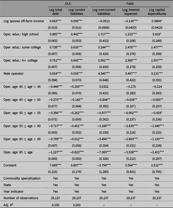
Note: standard errors in parentheses. ***P < 0.01, **P < 0.05, *P < 0.1.
Source: USDA Agricultural Resource Management Survey, 2007–2016. The sample includes family farms where the operator’s spouse does not work on-farm.
Table A2. Robustness of results to specification of second-stage IV regressions: log total debt
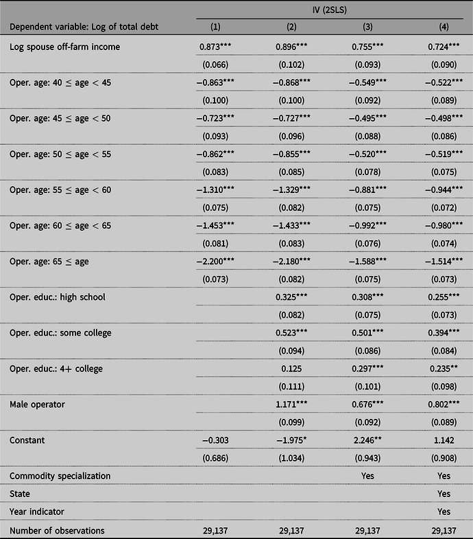
Note: standard errors in parentheses. ***P < 0.01, **P < 0.05, *P < 0.1.
Source: USDA Agricultural Resource Management Survey, 2007–2016. The sample includes family farms where the operator’s spouse does not work on-farm.
Table A3. Second-stage IV borrowing and investment regressions: spouse’s off-farm income from wages only
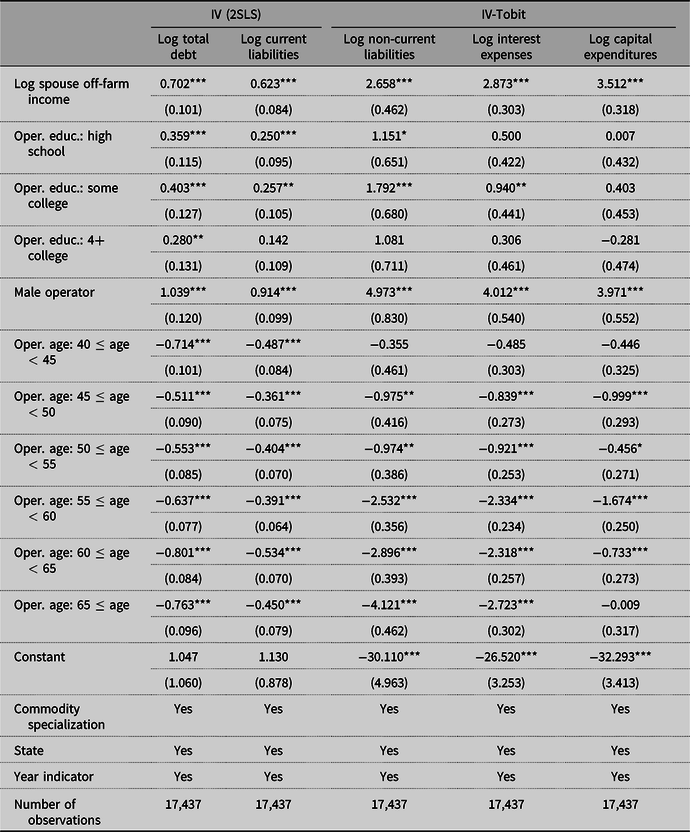
Note: standard errors in parentheses. ***P < 0.01, **P < 0.05, *P < 0.1.
Source: USDA Agricultural Resource Management Survey, 2007–2016. The sample includes family farms where the operator’s spouse does not work on-farm and the spouse earns a positive off-farm wage.


 Open access