


1. Introduction
Small family farms represent around 72% of farms globally (FAO, 2014).Footnote 1 In developing countries, increasing labor productivity among family farms is a pressing issue, as they face a sustained unfavorable productivity gap. As of 2013, the agricultural value-added per worker in the United States was 43 times higher, on average, than in developing countries in Africa and South America (Bank, Reference Bank2021). This gap comes from poor infrastructure and low human capital accumulation in the agricultural sector (Gutierrez, Reference Gutierrez2002). In developing countries, most family farms are small farms with limited access to developed markets, public support, and credit. They are located in rural areas with low investment in public goods, such as roads, electricity, and drinkable water, contributing to low agricultural productivity.
Technology adoption is an effective way to tackle this low productivity. Analyses of the 1960s Green Revolution find a positive and significant effect of implementing improved varieties of seeds on production (Evenson and Gollin, Reference Evenson and Gollin2003; Murgai, Reference Murgai2001). Other studies find indirect effects of technology adoption on productivity by accounting for a reduction in poverty in Bangladesh and Uganda (Kassie et al., Reference Kassie, Shiferaw and Muricho2011; Mendola, Reference Mendola2007), but technology adoption in a production process involves a series of complex steps (Doss, Reference Doss2006). First, the producer should be aware about the technology. Then, he or she should be willing to try it out, and finally, the producer should expect positive returns from using it to adopt it (Lambrecht et al., Reference Lambrecht, Vanlauwe, Merckx and Maertens2014). Therefore, many technical assistance programs include technology adoption as part of them to facilitate this complex process.
Technical assistance programs are based on knowledge transfer and provide training on new technologies to promote technology adoption. These programs are contingent on the needs of the community, but most of them include non-financial assistance—skills training, knowledge transfer, and consulting services—aiming to enhance agricultural production. In many Latin American countries, agriculture is an important productive sector (OECD/FAO, 2019) and their economic development strategies include technical assistance programs to improve agricultural production (Egas Yerovi and De Salvo, Reference Egas Yerovi and De Salvo2018). However, there is little research on the effect of technical assistance on agricultural production in these countries (Klerkx et al., Reference Klerkx, Landini and Santoyo-Cortés2016). Studies evaluating the impact of public technical assistance programs are scarce (OECD, 2015). There are no studies in the literature that model selection into the treatment of technical assistance, and there is no research on the heterogeneous effects of technical assistance.
Yet, impact variation is relevant for policy design purposes, as public investments can have a greater impact when focusing on the right population (Carneiro et al., Reference Carneiro, Heckman and Vytlacil2011). There are several studies on the heterogeneous effects of different social programs (Carneiro et al., Reference Carneiro, Heckman and Vytlacil2011; Carneiro et al., Reference Carneiro, Lokshin and Umapathi2017; Kline and Walters, Reference Kline and Walters2016; Maestas et al., Reference Maestas, Mullen and Strand2013; Morales et al., Reference Morales, Posso and Flórez2021; Noboa-Hidalgo and Urzúa, Reference Noboa-Hidalgo and Urzúa2012), but none of these studies focus on agricultural production. Hence, here, we seek to close that knowledge gap by analyzing the effect of technical assistance programs on agricultural production in Colombia. In this study, we model the probability that an agricultural unit receives technical assistance, estimate the Marginal Treatment Effect (MTE) of technical assistance on production, and describe the heterogeneous returns from technical assistance.
Following Heckman et al. (Reference Heckman, Urzua and Vytlacil2006), the MTE methodology extends the instrumental variables approach and allows us to test the existence of technical assistance heterogeneous effects. To do so, we use two instrumental variables: 1) exposure to armed conflict at the agricultural unit level and 2) planting cost. The first instrumental variable (IV) is based on a technical assistance program launched in 2012 by the national government. That technical assistance program targeted producers (agricultural units) located in areas with armed conflict. The second IV captures the opportunity cost of receiving technical assistance. To perform the analysis, we use micro data from the 2014 agricultural census in Colombia.
Based on our results, agricultural units that joined technical assistance programs increased their agricultural production value per hectare, on average, by 50.4% in comparison to agricultural units without technical assistance. We also find a heterogeneous effect of technical assistance. The smallest agricultural units that joined technical assistance programs increased their agricultural production value by 52%; this is more than 10% points in comparison to medium-sized agricultural units. In addition, we find that if the smallest agricultural units without technical assistance had joined the program, their agricultural production value would have increased by 45%. Therefore, our results show that technical assistance programs should target specifically the smallest units because there are opportunities to increase marginal benefits.
2. Technical Assistance and Agricultural Production
Technical assistance is a broad concept. In this study, agricultural extension and technical assistance refer to the same kind of activities focused on non-financial support to enhance agricultural production. Technical assistance includes training activities, knowledge transfer, and consulting services (DANE, 2014c). In some cases, agricultural units can receive technical assistance in more than one topic simultaneously, but most of the agricultural units in this study received training on good agricultural practices to minimize hazards in the harvest, packing, and transportation of fruits and vegetables (ICA, 2009).Footnote 2
The effect of technical assistance on agricultural production is also broad and varies from one study to another. Case studies in Malawi, India, Pakistan, and Paraguay reported positive and significant effects on agricultural production (Benyishay and Mobarak, Reference Benyishay and Mobarak2018; Bravo-Ureta and Evenson, Reference Bravo-Ureta and Evenson1994; Rosegrant and Evenson, Reference Rosegrant and Evenson1993), while in Indonesia, Feder, Murgai, and Quizon (Reference Feder, Murgai and Quizon2004) found no effect of farmer field schools on yield production, and Ragasa and Mazunda (Reference Ragasa and Mazunda2018) in Malawi found no effect of technical assistance on productivity. The main reason for this variation comes from unobserved characteristics and measurement error of technical assistance (Aker, Reference Aker2011; Evenson, Reference Evenson2001). Therefore, here we seek to control for the main source of endogeneity—the non-random selection process of agricultural units into technical assistance programs.
2.1. Agricultural Units and Technical Assistance Programs in Colombia
Located in South America, Colombia is the fourth largest economy in Latin America (OECD/UN/UNIDO, 2019). Five percentage of its gross domestic product (GDP) in 2014 comes from agriculture (DANE, 2018), and family farms dominate agricultural production. As of 2014, 65% of agricultural units in Colombia used family labor in their production process and 73% had <5 hectares (DANE, 2014a). In Colombia, an agricultural unit is a farm dedicated to produce agricultural products. It can be composed of a fraction, one, or more fields, but it has only one owner (producer), who is responsible for productive activities within the agricultural unit (DANE, 2014c). Therefore, most of the technical assistance programs are targeted to agricultural units.
As many small farms in developing economies, agricultural units in Colombia are labor-intensive and have little access to credit; 51% use fertilizers or pest controls, and only 11% applied for credit (DANE, 2014a). As a result of these and other limitations, Colombian labor productivity in the agricultural sector is 13 times less than in the United States (Bank, Reference Bank2021). Thus, improving agricultural productivity is a central issue in the local policy agenda, and technical assistance programs are one of the strategies being used.
The Colombian government is the leading provider of technical assistance in the country since the 1940s (OECD, 2015). In early stages of this economic developing strategy, technical assistance was provided by municipality management units that had autonomy to design projects with public funding. In the 2000s, the government created Centros Provinciales de Gestión Agroempresarial, local agricultural management centers that designed technical assistance projects and hired services from private companies. In 2007, the national government launched Agro Ingreso Seguro (AIS). As part of this national public program, the national government delivered subsidies directly to producers to buy technical assistance services (CNCA, 2008; Ley 1133 de 2007, 2007).
Under AIS, the government also implemented three different projects to provide technical assistance: 1) Asistencia Técnica Especial, focusing on small agricultural units in vulnerable conditions, 2) Asistencia Técnica Directa Rural, targeting small and medium agricultural units, and 3) Asistencia Técnica Gremial, directed to agricultural producers’ associations. Projects targeting agricultural units provided the following services: technology adoption, advice to choose productive activities, financial education, marketing, and producer organization capabilities. To access these services, each municipality designed a technical assistance plan and applied for funding. The central government selected the best projects and financed up to 80% of its total cost (MADR, 2014). This program operated during the period of study.
3. Data
This paper analyzes data from the Tercer Censo Nacional Agropecuario (CNA); an agricultural census conducted in 2014 that included 99% of rural Colombia. This census is the most updated and comprehensive source of information for studying the Colombian agricultural sector. The CNA collected data from agricultural units and non-agricultural units classified based on production activities developed at the time the survey was conducted. Agricultural units represent 41% of the total sample (919,512 observations). This analysis focuses on agricultural units with information about agricultural production in 2013. The final sample includes 191,588 agricultural units distributed across 1,118 municipalities throughout the country. Table 1 summarizes descriptive statistics of agricultural units included in the analysis.
Table 1. Characteristics of agricultural units in the sample
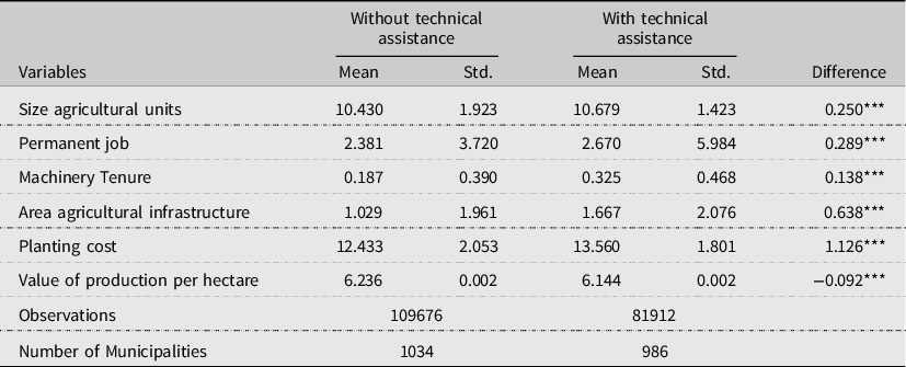
Notes: An agricultural unit is a business organization dedicated to the production of agricultural products. It can be composed by one, a fraction or more fields, but it has one and only one owner (producer). Most agricultural units have one household, but in some cases, there are multiple households within an agricultural unit. *** p < 0.01
The CNA also includes household characteristics and information about access to technical assistance programs. Technical assistance, the main independent variable in this analysis, is a discrete variable coded one if the agricultural unit received technical assistance in 2013, zero otherwise. Technical assistance is our treatment variable. In the sample, 33.7% of agricultural units received technical assistance. Agricultural units can receive technical assistance in several topics simultaneously. Most of the agricultural units that joined technical assistance programs received training on good agricultural practices, commerce and trading, and financial education (Appendix 1 shows all types of technical assistance reported in the CNA). Table 2 presents descriptive statistics of households at agricultural units included in the analysis.
Table 2. Characteristics of households and head of household at agricultural units
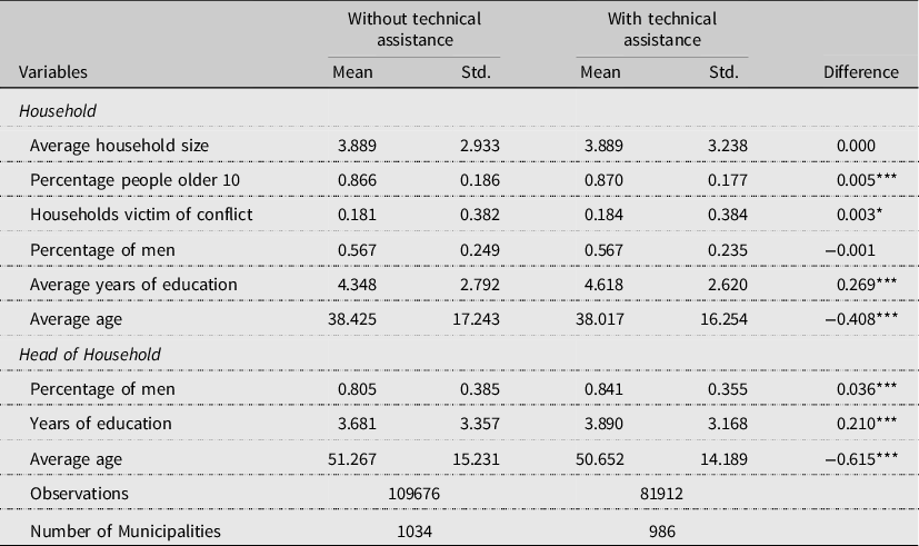
Notes: An agricultural unit is a business organization dedicated to the production of agricultural products. It can be composed by one, a fraction or more fields, but it has one and only one owner (producer). Most agricultural units have one household, but in some cases, there are multiple households within an agricultural unit. *** p < 0.01.
The outcome of interest in this paper is the value of agricultural production per cultivated area. To calculate this variable, we first multiplied the total quantity (in tons) of each crop by its price per ton in 2013. Then, we added up these monetary values from different crops to get an aggregate measure of production value. Finally, we divided this monetary value by the total cropped area in each agricultural unit. Equation (1) describes this calculation. Y is the value of agricultural production per hectare. ${q_j}$
is the total quantity in tons of each crop j.
${q_j}$
is the total quantity in tons of each crop j. ${p_j}$
is the price per ton of crop j, and A is the total cropped area in each agricultural unit. This measure makes possible to compare different crops across agricultural units and controls for heterogeneity in their size.
${p_j}$
is the price per ton of crop j, and A is the total cropped area in each agricultural unit. This measure makes possible to compare different crops across agricultural units and controls for heterogeneity in their size.
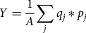 $$Y = {1 \over A}\sum\limits_j {{q_j}} \,{\rm{*}}\,{p_j}$$
Because the CNA does not include data on crop price, machinery cost, input cost, planting cost, or technical assistance cost, we used other data sources. To create a production value variable at agricultural unit level, we used data from: 1) the 2013 wholesale price information from the Sistema de Información de Precios y abastecimientos del Sector Agropecuario (SIPSA) and 2) the 2013 coffee base purchase price. SIPSA has data on 73 out of 484 crops included in the CNA data set, covering 21 out of 32 states in Colombia (Appendix 2 summarizes information for 73 crops). These data have prices for the most planted crops in Colombia, such as plantain, coffee, rice, cassava, corn, and potatoes. Finally, to estimate planting cost by crop, size, and location, we used data from the Red de Información y Comunicación del Sector Agropecuario Colombiano (Agronet, 2010). The resulting sample of crops and prices represents 72.32% of the total agricultural units with crop production information and 50.9% of the total area under cultivation.
4. Empirical Method
Agricultural units might adopt technical assistance due to factors we cannot observe, which can correlate with observed production. This issue is known as a selection bias problem. Our first solution to this bias problem is to use an IV approach, which allows us to identify causal inferences drawn from the effect of technical assistance on agricultural production. However, this solution ignores that agricultural units can know their result of receiving technical assistance based on their idiosyncratic characteristics before being selected. The existence of sorting on gains causes IVs to identify a local effect only. To address this concern, Heckman et al. (Reference Heckman, Urzua and Vytlacil2006) and Heckman and Vytlacil (Reference Heckman and Vytlacil2005) proposed a structural estimation of the MTE to improve the IV estimation. Following Carneiro et al. (Reference Carneiro, Heckman and Vytlacil2011) and Heckman et al. (Reference Heckman, Urzua and Vytlacil2006), this paper estimates the average treatment effect (ATE), average treatment of the treated (ATT), and average treatment of the untreated (ATUT) parameters and some policy simulations based on the MTE estimation.
Agricultural units choose to enroll in technical assistance programs based on the gains they anticipate from the program and unobserved factors such as productivity. Unobserved factors determine the selection into technical assistance treatment. Therefore, this is the primary source of endogeneity into the technical assistance variable. The MTE methodology allows controlling for this source of bias in the estimation by modeling the selection process into the treatment, in this case enrolling into technical assistance programs. This methodology is a general model of sorting on gains proposed by Heckman and Vytlacil (Reference Heckman and Vytlacil2005). In this paper, we model the selection into technical assistance, correcting any endogeneity bias explained by nonrandom selection into the treatment. Finally, to avoid any additional bias arising from the omission of relevant variables, we control for agricultural unit geographical location by including means of independent variables at the vereda level. Vereda is an administrative unit in Colombian similar to census tract in the United States. This procedure is equivalent to including vereda fixed effects (Malikov and Kumbhakar, Reference Malikov and Kumbhakar2014).
4.1. Structural Model
The following equations represent the potential crop production of agricultural units, depending upon receiving technical assistance or not:
 $${Y_1} = {\alpha _1} + X{\beta _1} + \;{U_1}\;\;\;$$
 $${Y_0} = {\alpha _0} + X{\beta _0} + {U_0}\;\;\;$$
Equation (2) illustrates the potential crop production value per hectare of agricultural units receiving technical assistance, while equation (3) represents crop production value per hectare for agricultural units not receiving assistance. In both cases, equations depend linearly on a set of observable characteristics, X, and unobservable characteristics, $U$
. Those unobserved characteristics can affect production differently depending on whether the farm is assisted; the difference of
$U$
. Those unobserved characteristics can affect production differently depending on whether the farm is assisted; the difference of ${U_1} - {U_0}$
represents the idiosyncratic heterogeneity of the technical assistance effect.
${U_1} - {U_0}$
represents the idiosyncratic heterogeneity of the technical assistance effect.
The decision to get technical assistance is discrete and depends on the unobserved latent variable I. Through a set of observed variables, Z, the selection equation (4) captures the technical assistance provision system’s bias toward producers with better production characteristics; this equation also models those factors that we do not see, which induces producers to join the program $\left( V \right)$
.
$\left( V \right)$
.
 $${D_{iv}} = 1\left[ {I = Z\gamma - V \ge 0} \right]\;\;\;$$
The Z vector includes exclusion restrictions that influence the enrollment into technical assistance, which in our case are exposure to conflict and planting cost; these characteristics are our IVs. The assumptions of the model are the following:
 $$\left( {Z,X} \right) \bot \left( {{U_1},{U_0},V} \right)$$
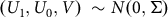 $$\left( {{U_1},{U_0},V} \right)\; \sim N\left( {0,{\rm{\Sigma }}} \right)$$
where $\Sigma = \left[ {\matrix{ {\sigma _0^2} {{\sigma _{1,0}}} {{\rho _1}} \cr {{\sigma _{1,0}}} {\sigma _1^2} {{\rho _2}} \cr {{\sigma _{v,0}}} {{\rho _2}} {\sigma _v^2} \cr } } \right]$
The central distributional assumption is that the errors ${U_1},{U_0},\;and\;V$
are jointly normally distributed (see Heckman and Vitlacyl, Reference Heckman and Vytlacil2005). The variance–covariance matrix
${U_1},{U_0},\;and\;V$
are jointly normally distributed (see Heckman and Vitlacyl, Reference Heckman and Vytlacil2005). The variance–covariance matrix $\;{\rm{\Sigma }}$
captures the existing relation between the different unobserved factors in structural and selection equations; this captures the selection bias in the model. It also collects the differential effect of selection bias on the potential outcomes.Footnote
3
$\;{\rm{\Sigma }}$
captures the existing relation between the different unobserved factors in structural and selection equations; this captures the selection bias in the model. It also collects the differential effect of selection bias on the potential outcomes.Footnote
3
4.2. Marginal Treatment Effect and Average Treatment Effect Estimation
The decision criteria can be expressed as $P\left( {z\gamma } \right) \ge {U_D}$
, where
$P\left( {z\gamma } \right) \ge {U_D}$
, where $P\left( {z\gamma } \right) = {\rm{\Phi }}\left( {z\gamma } \right)$
by the normality assumption.
$P\left( {z\gamma } \right) = {\rm{\Phi }}\left( {z\gamma } \right)$
by the normality assumption. ${U_D}$
is the cumulative probability of observing a particular level of V. By construction,
${U_D}$
is the cumulative probability of observing a particular level of V. By construction, ${U_D}\sim Unif\left( {0,1} \right)$
. The MTE is defined as the partial derivative of the potential outcome with respect to the probability of being treated, conditional in a fixed value of the observed set and
${U_D}\sim Unif\left( {0,1} \right)$
. The MTE is defined as the partial derivative of the potential outcome with respect to the probability of being treated, conditional in a fixed value of the observed set and ${U_D}$
:
${U_D}$
:
 $$MTE = \;{{\partial E\left( {Y{\rm{|}}X = x,P = p} \right)} \over {\partial p}}\;\;\;$$
Intuitively, in equation (7), the MTE measures change in the production due to marginal increments in the probability of receiving technical assistance. Under this definition, equations (2–4), and the assumptions of the model, the following equation (8) represents the MTE:
 $$MTE = {\alpha _1} - {\alpha _0} + x\left( {{\beta _1} - {\beta _0}} \right) + \left( {{\rho _1} - {\rho _0}} \right){{\rm{\Phi }}^{ - 1}}\left( {{u_D}} \right)\;\;\;$$
Parameters ${\rho _1}$
and
${\rho _1}$
and ${\rho _0}$
represent the covariance between the unobservables of selection equation with unobservables of outcome equations for the treated and untreated units, respectively. We get
${\rho _0}$
represent the covariance between the unobservables of selection equation with unobservables of outcome equations for the treated and untreated units, respectively. We get ${\alpha _1},{\alpha _0},{\beta _1},{\beta _0},\;{\rho _1},{\rho _0}$
by estimating the system of equations (2–4) by maximum likelihood (Brave and Walstrum, Reference Brave and Walstrum2014). As demonstrated by Heckman and Vytlacil (Reference Heckman and Vytlacil2005), the treatment effects ATE, ATT, and ATUT are weighted averages of the MTE over the distribution of
${\alpha _1},{\alpha _0},{\beta _1},{\beta _0},\;{\rho _1},{\rho _0}$
by estimating the system of equations (2–4) by maximum likelihood (Brave and Walstrum, Reference Brave and Walstrum2014). As demonstrated by Heckman and Vytlacil (Reference Heckman and Vytlacil2005), the treatment effects ATE, ATT, and ATUT are weighted averages of the MTE over the distribution of ${U_D}$
; therefore, their estimation is resumed in equation (9):
${U_D}$
; therefore, their estimation is resumed in equation (9):
 $${\Delta ^{TE}}\left( x \right) = \mathop \int \limits_0^1 MTE\left( {x,{u_D}} \right){h_{TE}}\left( {x,{u_D}} \right)d{u_D}$$
where ${h_{TE}}\left( {x,{u_D}} \right)$
is the weight for each treatment effect. When ATT > ATE > ATUT, the treated units invest in technical assistance because they know that they will benefit more from it.
${h_{TE}}\left( {x,{u_D}} \right)$
is the weight for each treatment effect. When ATT > ATE > ATUT, the treated units invest in technical assistance because they know that they will benefit more from it.
The MTE estimation also allows simulating the returns of policies for the marginal individual, the one indifferent between enrolling or not into a specific treatment. The Marginal Policy Relevant Treatment Effect (MPRTE) measures the average return of a policy for those induced to enroll into the treatment by increasing in the margin the probability of enrollment (equation 9 for a different set of weights) (Heckman and Vytlacil, Reference Heckman and Vytlacil2001). This parameter sheds light on the returns of programs’ expansion and compares what type of expansion generates more returns: a homogeneous increase in the program or one that favors the more prone to enroll.
4.3. Instrumental Variables
This analysis uses exposure to conflict and planting cost as instrumental variables. Colombia has a long history of armed conflict in which Marxist guerrillas have been fighting the government in an attempt to gain political power. Therefore, the CNA includes a question about exposure to armed conflict in the household characteristics section.Footnote 4 For this study, we created a measure of exposure to conflict at agricultural unit level. This variable shows the percentage of households affected by armed conflict within the agricultural unit before 2013. We used data on forced displacement, land dispossession, and land abandonment reported by every household within each agricultural unit to calculate this variable.
Armed conflict in Colombia takes place in rural areas. In response to this situation, the technical assistance national public program—AIS—included a project designed for producers in vulnerable conditions such as armed conflict. Asistencia Técnica Especial provided comprehensive support and knowledge transfer to small agricultural units. Given that one of the most frequent forms of victimization in rural areas is forced displacement, this involuntary movement of people is an important determinant of the probability to receive technical assistance. Projects focusing on rural households exposed to conflict are likely to improve their production techniques, but the fact that a household is exposed to armed conflict is an exogenous shock, unlikely to be desired or anticipated by the household. Therefore, exposure to conflict is plausibly independent of the agricultural unit unobserved characteristics. The only way that exposure to the conflict could affect production is through inducing agricultural units to get technical assistance based on the targeting mechanisms of the project Asistencia Técnica Especial. Table 3 (First stage) illustrates the statistically significant relationship between forced displacement and the propensity of technical assistance.
Table 3. First stage and selection equation
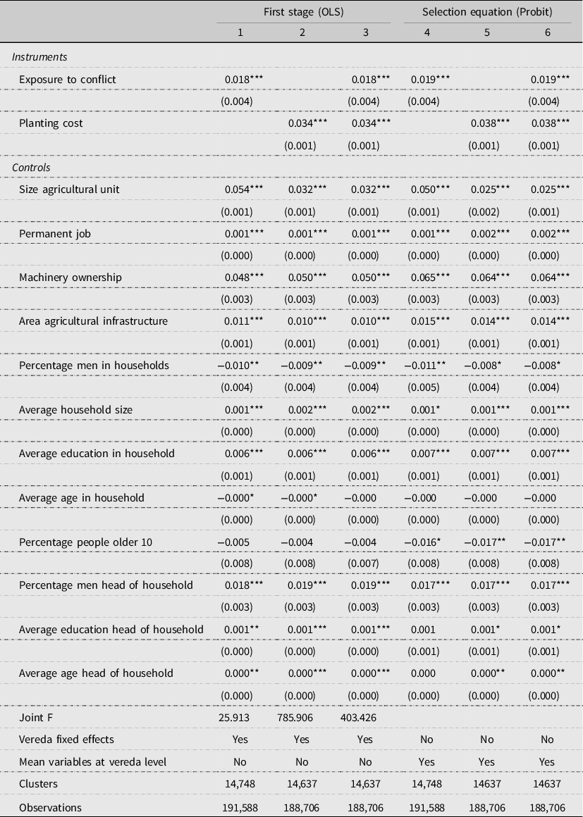
Notes: Standard errors clustered by vereda level. Dependent variable is a dummy for receiving technical assistance. For a threshold tau = 10%, all instruments reject the null hypothesis of weak instrument. *** p < 0.01, ** p < 0.05, * p < 0.10
The other instrument captures one of the most critical market costs that agricultural producers face, planting cost. Technical assistance provides technology that can reduce production costs, so agricultural units facing higher planting costs may be induced to join technical assistance programs. However, agricultural units cannot affect the market planting cost because it is a market result subject to the evolution of input prices and agricultural services. In addition, the agricultural sector is highly competitive and we enhanced the exogeneity of this IV by using the costs in other markets for the same crop. To compute the planting cost in unit i, we used the same crop average cost in all other states. Finally, when we estimated IV regressions with exposure to conflict and planting cost IV separately, the local effects’ magnitudes are similar. Table 3 (First stage) shows a positive and statistically significant correlation between planting cost and technical assistance propensity.
Based on our first stage results, the instruments used for this estimation are relevant to explain the decision to participate in a technical assistance program. The first-stage F-statistic, proposed by Montiel Olea and Pflueger (Reference Montiel Olea and Pflueger2013), rejects the null hypothesis of weak instruments. Table 3 also reports results of the selection equation estimation (equation 4). This regression captures the relation between technical assistance and our instruments using a probit model. The estimation of equation (4) is equivalent to the first stage of a two-stage least squares model. Our instruments are statistically significant in all specifications, and the t-statistics are sizeable. Results from the selection equation display a positive relationship between planting cost and the probability of adopting technical assistance, and a positive association between exposure to conflict and the probability of adopting technical assistance.
5. Results
To estimate the effect of technical assistance on agricultural production value, we estimated the MTE, ATE, ATT, and the ATUT. We also estimated the MPRTE; a policy simulation that measures the effect of increasing the probability of treatment. Finally, for the sake of comparison, we estimated ordinary least squares (OLS), instrumental variables (IV) and two-stage least squares (2SLS) models as well. The 2SLS estimation is also useful for testing our instruments’ validity.
5.1. OLS, IV, and 2SLS Estimations
Table 4 shows estimations for OLS, IV, and 2SLS using fixed effects and Eicker–Huber–White standard errors clustered by vereda. Column (1) reports results for the OLS estimation. Columns (2) and (3) present IV results for the following instrumental variables: exposition to conflict and planting cost. Column (4) shows 2SLS results using both instruments together. We also performed a standard over-identification restriction test (Hassen J) in the regression with both instruments.Footnote 5 Under the null hypothesis, instruments are valid because they are uncorrelated with the error term. Based on our results, we do not reject the hypothesis that all IVs are valid, given its uncorrelation with the structural equation’s regression error. Therefore, we argue that exposure to conflict and planting cost are independent of the agricultural unit’s unobserved characteristics.
Table 4. OLS, IV, and 2SLS regressions
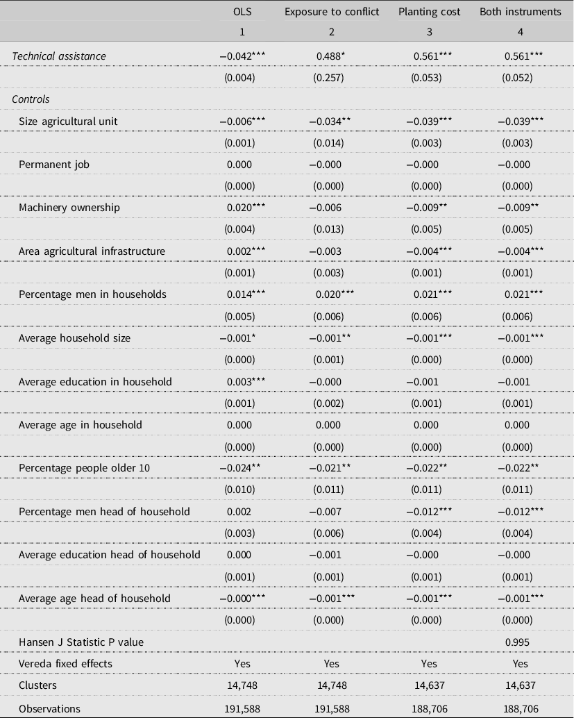
Notes: Standard errors clustered by vereda level. * p < 0.1, *** p < 0.01.
Columns (2) and (3) show results for models exactly identified for each IV separately. Using exposure to conflict (column 2), the effect of technical assistance for those induced to participate in the program as a result of being exposed to armed conflict is 48%. Using planting cost (column 3), the effect is 56%. Both of these results are statistically significant, so agricultural units induced to participate in technical assistance programs increase their production value per hectare between 48 and 56%. These findings are consistent with previous studies in Argentina reporting yield increments between 46 and 58% after joining technical assistance programs (Cerdán-Infantes et al., Reference Cerdán-Infantes, Maffioli and Ubfal2008), and results from a meta-analysis of 292 publications reporting median rates of return to extension efforts of 58% (Alston et al., Reference Alston, Chan-Kang, Marra, Pardey and Wyatt2000). However, in Colombia, they are particularly relevant because improvement of living conditions in rural areas is a priority, and technical assistance provides a mechanism to increase agricultural productivity, thus rural population income.
Results from the 2SLS estimation in column (4) also show a positive local effect of technical assistance on agricultural production value. Using both instruments, joining a technical assistance program increases production value per hectare by 56%. Coefficients on some control variables are also statistically significant. However, they should be interpreted with caution because in this analysis we control for endogeneity only in our main independent variable—technical assistance. There is a negative relationship between average age of the head of household and agricultural production value per hectare. Previous studies suggested that this relationship is mediated by the risk of aversion (Picazo-Tadeo and Wall, Reference Picazo-Tadeo and Wall2011). Hence, the older the head of household, the less likely he or she is to adopt new technologies (Dercon and Christiaensen, Reference Dercon and Christiaensen2011). This negative relationship implies that technical assistance programs should factor the age of the head of household in their design to improve results.
There are other interesting correlations between some covariates and the dependent variable. The size of the agricultural unit has a negative correlation with the agricultural production value per hectare. The direction of this result is expected because the dependent variable is the value of the production per hectare. The size of the household has a negative correlation with the dependent variable as well. This result could be capturing the negative relationship between fertility/family size and income (Ashraf et al., Reference Ashraf, Weil and Wilde2013; Schultz, Reference Schultz1997). There is also a negative correlation between the percentage men head of household and agricultural production value. Nevertheless, there is a positive correlation of the dependent variable with the percentage of men in the household. These results bring in the discussion about gender differences in agricultural productivity (Peterman et al., Reference Peterman, Quisumbing, Behrman and Nkonya2011; Quisumbing, Reference Quisumbing1996; Slavchevska, Reference Slavchevska2015; Udry, Reference Udry1996), a very relevant and interesting topic that remains material for future research.
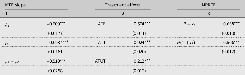
5.2. MTE Estimation
Our main model is a parametric estimation of the equation system (2), (3), and (4), which in turn allows the estimation of our main evaluation parameter: the MTE (see equation 8). The MTE describes the heterogeneity in the return of technical assistance on agricultural production value per hectare. Table 5, column (1), presents the result of a test of heterogeneity in the returns. We test if the slope of the MTE is statistically equal to zero, $\left( {{\rho _1} - {\rho _0}} \right) = 0$
. Based on our results, we reject the hypothesis at the 95% confidence level. Therefore, there is heterogeneity in the returns of technical assistance on agricultural production value per hectare.
$\left( {{\rho _1} - {\rho _0}} \right) = 0$
. Based on our results, we reject the hypothesis at the 95% confidence level. Therefore, there is heterogeneity in the returns of technical assistance on agricultural production value per hectare.
Table 5. MTE estimation, treatment effects, and policy estimates
Notes: Standard errors are calculated with bootstrap (100 repetitions). Control variables not reported in this table, but included in estimations, are agricultural production unit characteristics and characteristics of households within the agricultural unit. *** p < 0.01
Figure 1 illustrates the MTE estimation and shows a sizable heterogeneity of returns. The horizontal axis in Figure 1 is a function of the probability of selection into treatment. Individuals with a high probability of selection have a higher return of enrolling into technical assistance programs. Individuals with a low probability of selection have lower returns. On the one hand, we find a positive return of 115% for producers that, given their unobservable characteristics, are the most likely to enroll in technical assistance programs (percentile 10 of the distribution of ${u_D}$
in equation 7). On the other hand, we find a negative return of 15% for producers that given their unobservable characteristics, have the lowest probability to enroll in technical assistance programs (percentile 90 of the distribution of
${u_D}$
in equation 7). On the other hand, we find a negative return of 15% for producers that given their unobservable characteristics, have the lowest probability to enroll in technical assistance programs (percentile 90 of the distribution of ${u_D}$
). This pattern of selection on expected gains has been previously studied (Heckman and Vytlacil, Reference Heckman and Vytlacil2005) and explains the positive sorting gains observed in our results.
${u_D}$
). This pattern of selection on expected gains has been previously studied (Heckman and Vytlacil, Reference Heckman and Vytlacil2005) and explains the positive sorting gains observed in our results.
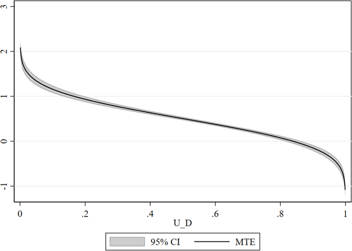
Figure 1. MTE estimated.
Notes: The MTE is calculated in the average of the observed characteristics. Confidence bands are calculated using delta method and standard errors clustered by vereda level. The vertical axis shows the effect of technical assistance for each evaluation point of ${U_D}$
between [0.01,0.99] in steps of 0.01 (Brave and Walstrum, Reference Brave and Walstrum2014).
${U_D}$
between [0.01,0.99] in steps of 0.01 (Brave and Walstrum, Reference Brave and Walstrum2014).
Column (2) reports results for standard treatment effects. The ATE of enrolling in a technical assistance program is an increase of 50.4% of agricultural production value per hectare, relative to the situation without technical assistance. This result is consistent with rates of return to technical assistance, greater than or equal to 50%, found in previous studies in other 17 countries (Evenson, Reference Evenson, Swanson, Bentz and Sofranko1997). Specifically for Latin America, rates of return to technical assistance could reach up to 80% (Evenson, Reference Evenson2001). In the same column, the ATT and ATUT point out a positive sorting on gains in technical assistance adoption by agricultural producers. Agricultural units enrolled in technical assistance programs have greater returns to technical assistance, in terms of agricultural production value per hectare (92.4), than those who did not enroll (21.2), in the counterfactual scenario in which they would have enrolled. Therefore, it is likely that beneficiaries of technical assistance services enrolled in the programs because they had the expectation that their productivity would increase.
Using the results from the ATE estimation, we also compute a back to the envelope calculation of the average cost–benefit ratio of providing technical assistance. This is an approximation because we have aggregated information on cost and potential beneficiaries. Using aggregated information on the total technical assistance investment, potential beneficiaries, and our estimation of technical assistance enrollment rate, we find that the average amount of subsidies provided by the Colombian government, in 2013 to get technical assistance, was around 257 USD.Footnote 6 The average agricultural production value per hectare in our sample is 1467 USD, so an ATE of 50.4 percentage implies an average increase of 778 USD. Therefore, the cost–benefit ratio is 3, (778 /257); for every 1 USD spent on technical assistance, the producer receives an increase in agricultural production of 3 USD. Based on our results, technical assistance is a cost-effective strategy to boost agricultural productivity.
To verify the validity of the instruments and the fact that specific subpopulations do not drive our results, we perform some robustness exercises. Regarding the validity of the instruments, we use the median and weighted average planting cost for the same crop in other states. Our results are robust to these changes, and in all over-identified regressions, the instruments are valid in terms of the identifying restriction test (Hansen J Statistic) (Results available in Appendix 3). Because the National Federation of Coffee Growers has an extensive technical assistance program and reaches most coffee producers in Colombia, we test if coffee producers are driving our results. To do so, we exclude them from the sample and re-estimate previous exercises. We find that technical assistance has a positive effect on agricultural production value per hectare in places where coffee is not the main crop. The estimated coefficients are larger than the ones obtained for the whole sample (Results available in Appendix 4). Therefore, our main result holds for a sample of producers who are not coffee growers. There are positive effects of technical assistance in sectors different to coffee, and our findings are robust to changes in the set of instruments.
5.3. Technical Assistance Policies Simulations
In addition to traditional impact evaluation parameters, ATE, ATT, and ATUT, the MTE estimation allows the simulation of policy responses for the marginal individual. The Marginal Policy Relevant Treatment Effect (MPRTE) measures the effect of increasing marginally the probability of treatment (Carneiro et al., Reference Carneiro, Heckman and Vytlacil2011; Heckman and Vytlacil, Reference Heckman and Vytlacil2005), for instance, the impact of a small increase in the probability of enrolling in technical assistance on agricultural production value per hectare. Based on our results, technical assistance has a positive impact on agricultural production value. Hence, we estimate the effect of two different policies: one policy that homogeneously expands technical assistance program coverage and another that proportionally increases the probability of enrolling in technical assistance programs. The first policy increases the probability of obtaining technical assistance equally among producers, while the second policy favors producers who are more likely to receive technical assistance. Linking these policies to the selection model presented in equation (4), we can express them as changes in the propensity score, $P + \alpha $
and
$P + \alpha $
and $\;P\left( {1 + \alpha } \right)$
, respectively.
$\;P\left( {1 + \alpha } \right)$
, respectively.
Table 5, column (3), presents the MPRTE estimates for technical assistance policies. First, we estimate the effect of increasing homogeneously the probability of receiving technical assistance, $P + \alpha $
. We find that increasing one percentage point the probability of enrollment into technical assistance increases agricultural production value per hectare by 63.8% for the marginal individual. Then, we estimate the effect of increasing proportionally the probability of receiving technical assistance,
$P + \alpha $
. We find that increasing one percentage point the probability of enrollment into technical assistance increases agricultural production value per hectare by 63.8% for the marginal individual. Then, we estimate the effect of increasing proportionally the probability of receiving technical assistance, $P\left( {1 + \alpha } \right)$
. In this case, we find that if the probability of enrollment increases 1%, agricultural production value increases by 50.6% for the marginal individual. Therefore, a policy that uniformly increases the coverage of technical assistance is more effective than one that increases coverage to producers who, in the baseline, had more chances of receiving technical assistance.
$P\left( {1 + \alpha } \right)$
. In this case, we find that if the probability of enrollment increases 1%, agricultural production value increases by 50.6% for the marginal individual. Therefore, a policy that uniformly increases the coverage of technical assistance is more effective than one that increases coverage to producers who, in the baseline, had more chances of receiving technical assistance.
5.4. Heterogeneity by Agricultural Unit Size
Previous estimations assume that technology of production is homogenous among producers. However, this assumption might be restrictive and can hide differences in technical assistance performance across agricultural production units. Therefore, we re-estimate the model, dividing our sample by quartiles of land size. Table 6 presents the treatment effects and policy parameters by samples according to the agricultural unit size. The ATE exhibits U shape results depending on agricultural unit size. On average, the smallest and largest units would benefit the most from joining technical assistance programs. These results are relevant for public policy strategies focusing on higher returns of investment.
Table 6. Heterogeneous effect by agricultural unit size

Notes: Ha refers to hectares. Standard errors calculated with bootstrap (100 repetitions). Control variables not reported in this table, but included in estimations, are agricultural production unit characteristics and households within the unit. *** p < 0.01, ** p < 0.05, * p < 0.1
Agricultural units with more than 11 hectares have the highest ATT effect, and in all cases, the ATT is higher than the ATUT. These results support the existence of selection on expected gains. This type of sorting pattern is more important for larger agricultural units because they are probably the most productive ones. Another interesting finding is that the ATUT is the highest for the smallest units. Therefore, in the counterfactual scenario in which non-treated small units would have received technical assistance, they would have increased their production value by 45%. This result contributes to the discussion of the role of scaling technical assistance programs. There are concerns in the literature about whether those who are getting assistance are the ones who would benefit most from it (Anderson and Feder, Reference Anderson and Feder2007; Hellin, Reference Hellin2012). Our estimation results show that agricultural policies should target technical assistance programs on the smallest units, for which there are ample opportunities for the marginal benefits.
6. Conclusions
In this paper, we find that technical assistance has the potential to increase agricultural production. Technical assistance has a large and positive average effect on the value of production per hectare, 50.4%. This result is consistent with the average return of technical assistance investments found in many developing countries (Anderson and Feder, Reference Anderson and Feder2007; Evenson, Reference Evenson, Swanson, Bentz and Sofranko1997). One of our main findings is that this effect is not homogeneous through all units. We find that the marginal effect for agricultural units with a higher probability of being treated could reach 115%; nevertheless, the effect could be negative for those with the smallest probability of treatment. In line with this evidence, the ATT (92%) is far greater than the ATUT (21%), revealing the existence of sorting on gains. Agricultural units that are induced to the treatment are the ones with higher expectations of the effect of technical assistance in their production.
This paper also explores the effect of technical assistance programs for victims of armed conflict. In the literature, there is no evidence on the positive impact of policies directed to rural populations affected by armed conflict; nevertheless, there is evidence of the negative effect of conflict on food security in developing countries (Jeanty and Hitzhusen, Reference Jeanty and Hitzhusen2006). In a similar study, Segovia (Reference Segovia2017) finds negative effects of armed conflict on Colombia’s food security. In terms of policy implications, our findings stress the benefit of maintaining and expanding technical assistance programs and the need to implement policies targeting armed conflict zones. Our results provide evidence that policies directed to farms affected by violence are an effective strategy to increase agricultural productivity, increase income, and help victims overcome poverty. Finally, our findings reveal that there is still a considerable margin for technical assistance program extensions since the ATUT is still a considerable 21%.
Acknowledgments
We would like to thank Camilo Bohorquez-Penuela for his helpful feedback on multiple drafts of this paper. We are also grateful to the editor and three anonymous reviewers for their constructive comments and suggestions. Thank you as well to Johanna Yepes for her support to advance this research project. All remaining errors are our own.
Competing Interests
Nicolás Arturo Torres Franco has received a scholarship from Universidad EAFIT. Eleonora Dávalos and Leonardo Fabio Morales declare none.
Data Availability Statement
The data that support the findings of this study are openly available in https://github.com/eleodavalos/heterogeneousTA.
Funding Statement
This research received no specific grant from any funding agency, commercial or not-for-profit sectors.
Appendix 1. Percentage of agricultural units that received technical assistance by topic

Notes: Percentage of agricultural units that reported technical assistance services by topic. Calculated based on DANE (2014a) data.
Appendix 2. Descriptive statistics at crop level

Notes: * p < 0.1, ** p < 0.05, *** p < 0.01. Table A2 shows the 73 crops for which we have price information are mostly for basic consumption. Most of them are transitory fruits and crops with high relevance for the agricultural production of Colombia representing 61.85% of the planted area of the country. The more important crops in terms of planted area and number of agricultural units that produce them are the Plantain and Coffee. This is also evidenced of the percentage of assisted agricultural units that cultivate them. Total States and Mean Price are obtained from states with price and crop production information. Percentage area planted, Total agricultural units, percentage agricultural units with or without technical assistance. The difference in average yield is calculated as the difference in the value of production per hectare between agricultural units with technical assistance and agricultural units without technical assistance. Absolute value of t statistics is presented in parenthesis.

Appendix 3. 2SLS Robustness checks

Notes: Standard errors clustered by vereda level. In columns 1 and 2, we use the median and weighted average planting cost for the same crops in other states. In the case of the weighted average, we use importance weights according to the similitude of the crops’ composition between the state in which a unit is located and any other state. In column 4, we use agricultural unit own plating cost. * p < 0.1, *** p < 0.01.
Appendix 4. Robustness coffee production

Notes: Standard errors are calculated with bootstrap (100 repetitions). Control variables not reported in this table, but included in estimations, are agricultural production unit characteristics and characteristics of households within the agricultural unit. *** p < 0.01.


 Open access