


1 Introduction
Hot-image effect is one of the predominant threats to large-aperture optics in high power laser systems[Reference Hunt, Manes and Renard1–Reference Yang, Liu, Gao, Miao and Zhu17]. Typically, hot images in the main amplifier section appear periodically on alternating plates. In 1993, Hunt et al. analyzed the formation process of hot images that is akin to holographic imaging [Reference Hunt, Manes and Renard1]. Xie et al. derived a more comprehensive analytic expression about the variation of hot-image intensity with the properties of defects and
 $B$
integral in 2004[Reference Xie, Jing, Zhao, Su, Wang and Peng5, Reference Xie, Zhao, Su, Jing, Wang and Peng6]. The intensity magnification is given as
$B$
integral in 2004[Reference Xie, Jing, Zhao, Su, Wang and Peng5, Reference Xie, Zhao, Su, Jing, Wang and Peng6]. The intensity magnification is given as
 $1+(1+\unicode[STIX]{x1D70F}^{2}-2\unicode[STIX]{x1D70F}\cos \unicode[STIX]{x1D703})B^{2}+2\unicode[STIX]{x1D70F}B\sin \unicode[STIX]{x1D703}$
. In 2009, Li et al. proved that an intensity minimum exists during hot-image formation process[Reference Li, Zhao, Peng and Cai8]. Scholars also studied the impacts of other parameters on the hot-image distribution, including the thickness of nonlinear plate, wavelength, damage size, as well as the joint effect of multiple defects[Reference Li, Zhao, Peng and Ye9–Reference You, Zhang, Zhang, Sun and Zhu12]. In 2016, Manes et al. summarized the formation mechanisms and managements of hot images in the whole system[Reference Manes, Spaeth, Adams, Bowers, Bude, Carr, Conder, Cross, Demos, Di Nicola, Dixit, Feigenbaum, Finucane, Guss, Henesian, Honig, Kalantar, Kegelmeyer, Liao, MacGowan, Matthews, McCandless, Mehta, Miller, Negres, Norton, Nostrand, Orth, Sacks, Shaw, Siegel, Stolz, Suratwala, Trenholme, Wegner, Whitman, Widmayer and Yang13]. In general, research results in the past years indicate that hot images are closely related with the properties of incident beams, optical elements as well as defects.
$1+(1+\unicode[STIX]{x1D70F}^{2}-2\unicode[STIX]{x1D70F}\cos \unicode[STIX]{x1D703})B^{2}+2\unicode[STIX]{x1D70F}B\sin \unicode[STIX]{x1D703}$
. In 2009, Li et al. proved that an intensity minimum exists during hot-image formation process[Reference Li, Zhao, Peng and Cai8]. Scholars also studied the impacts of other parameters on the hot-image distribution, including the thickness of nonlinear plate, wavelength, damage size, as well as the joint effect of multiple defects[Reference Li, Zhao, Peng and Ye9–Reference You, Zhang, Zhang, Sun and Zhu12]. In 2016, Manes et al. summarized the formation mechanisms and managements of hot images in the whole system[Reference Manes, Spaeth, Adams, Bowers, Bude, Carr, Conder, Cross, Demos, Di Nicola, Dixit, Feigenbaum, Finucane, Guss, Henesian, Honig, Kalantar, Kegelmeyer, Liao, MacGowan, Matthews, McCandless, Mehta, Miller, Negres, Norton, Nostrand, Orth, Sacks, Shaw, Siegel, Stolz, Suratwala, Trenholme, Wegner, Whitman, Widmayer and Yang13]. In general, research results in the past years indicate that hot images are closely related with the properties of incident beams, optical elements as well as defects.
In order to ensure the safe operation of the system, solutions are proposed to circumvent this threat. The spatial filter is a conventional method to suppress hot images in the main amplifier section, which is used to remove those Fourier spectrum components that would experience high gains[Reference Peng, Zhao, Xie, Ye, Wei, Su and Zhao14, Reference Zhang, Zhang, Jiao, Sun, Liu and Zhu15]. In 2017, Yang et al. put forward a prejudgement strategy of hot images with the inversed properties of the pure amplitude defects[Reference Yang, Liu, Gao, Miao and Zhu16, Reference Yang, Liu, Gao, Miao and Zhu17]. However, complex-amplitude defects of tens of microns can still induce hot images. Weak disturbances of the diffraction field induced by these defects can hardly be cleaned with the spatial filter. Therefore, a more practical solution is needed to further reduce the damage of hot images.
In this paper, formation process of hot images induced by defects of tens of microns is analyzed theoretically and numerically. Results show that the hot image can be precisely calculated with the extracted intensity oscillation of the diffraction ring on the front surface of the nonlinear plate. The gradient direction matching (GDM) method is employed to detect diffraction rings as the gradient direction is the most robust information extracted from the diffraction ring images[Reference Paglieroni and Eppler18–Reference Chen, Kegelmeyer, Liebman, Thaddeus Salmon, Tzeng and Paglieroni20]. Analysis of recognizing simulated diffraction rings shows that the conventional criterion that the overlap ratio should be smaller than 50% is not enough[Reference Yang, Liu, Gao, Miao and Zhu16, Reference Yang, Liu, Gao, Miao and Zhu17, Reference Chen, Kegelmeyer, Liebman, Thaddeus Salmon, Tzeng and Paglieroni20]. Hot images induced by those closely spaced defects and the defects that are far apart from each other can both be directly prejudged as long as the regular structure of central light spot in the diffraction ring is still reserved. Image compression and cluster analysis are used to make the GDM method more robust and practical in recognizing actually collected diffraction images. Results show that hot images induced by defects of tens of microns can be directly prejudged without redundant information.
2 Relationship between diffraction rings and hot images
Hot-image formation process is analyzed theoretically and numerically to investigate the relationship between diffraction rings and hot images. Disk amplifiers are periodically arrayed in the Brewster angle. To simplify analysis, these nonlinear plates are all set perpendicular to the beam propagation direction. Gain and loss characteristics are also ignored in the subsequent analysis, which is shown schematically in Figure 1.
The incident beam is set as the plane wave
 $U=A\exp (\text{i}kz)$
that propagates along the
$U=A\exp (\text{i}kz)$
that propagates along the
 $z$
-axis, where
$z$
-axis, where
 $A$
is the amplitude,
$A$
is the amplitude,
 $\unicode[STIX]{x1D706}$
is the wavelength and
$\unicode[STIX]{x1D706}$
is the wavelength and
 $k$
is the wavenumber. The beam is modulated by a defect on the scatter plane
$k$
is the wavenumber. The beam is modulated by a defect on the scatter plane
 $(x_{1},y_{1})$
. Transmittance function of the plane can be described as
$(x_{1},y_{1})$
. Transmittance function of the plane can be described as
 $$\begin{eqnarray}t_{0}(x_{1},y_{1})=\left\{\begin{array}{@{}ll@{}}\unicode[STIX]{x1D70F}\cdot \exp (\text{i}\unicode[STIX]{x1D703})\quad & \text{damage site,}\\ 1\quad & \text{others,}\end{array}\right.\end{eqnarray}$$
where
 $\unicode[STIX]{x1D70F}$
is the amplitude modulation coefficient and
$\unicode[STIX]{x1D70F}$
is the amplitude modulation coefficient and
 $\unicode[STIX]{x1D703}$
is the phase modulation coefficient. The complementary function is given as
$\unicode[STIX]{x1D703}$
is the phase modulation coefficient. The complementary function is given as
 $t(x_{1},y_{1})=1-t_{0}(x_{1},y_{1})$
. After propagating in free space for a distance
$t(x_{1},y_{1})=1-t_{0}(x_{1},y_{1})$
. After propagating in free space for a distance
 $d_{0}$
from the scatter plane, the diffraction field on the front surface
$d_{0}$
from the scatter plane, the diffraction field on the front surface
 $(x_{2},y_{2})$
of the nonlinear plate can be described with the Fresnel diffraction integral equation and given as
$(x_{2},y_{2})$
of the nonlinear plate can be described with the Fresnel diffraction integral equation and given as
 $$\begin{eqnarray}\displaystyle & & \displaystyle U(x_{2},y_{2})=\frac{A\exp (\text{i}kd_{0})}{\text{i}\unicode[STIX]{x1D706}d_{0}}\nonumber\\ \displaystyle & & \displaystyle \qquad \times \,\left\{\iint \exp \left\{\!\frac{\text{i}k}{2d_{0}} [(x_{2}-x_{1})^{2}\right.\right.\nonumber\\ \displaystyle & & \displaystyle \qquad \left.+\,(y_{2}-y_{1})^{2} ]\vphantom{\displaystyle \iint }\!\right\}\,\text{d}x_{1}\,\text{d}y_{1}\nonumber\\ \displaystyle & & \displaystyle \qquad -\,\iint t(x_{1},y_{1})\exp \left\{\!\frac{\text{i}k}{2d_{0}} [(x_{2}-x_{1})^{2}\right.\nonumber\\ \displaystyle & & \displaystyle \qquad \left.\left.+\,(y_{2}-y_{1})^{2} ]\vphantom{\displaystyle \iint }\!\right\}\,\text{d}x_{1}\,\text{d}y_{1}\right\}\nonumber\\ \displaystyle & & \displaystyle \quad =U_{R}+U_{0}.\end{eqnarray}$$
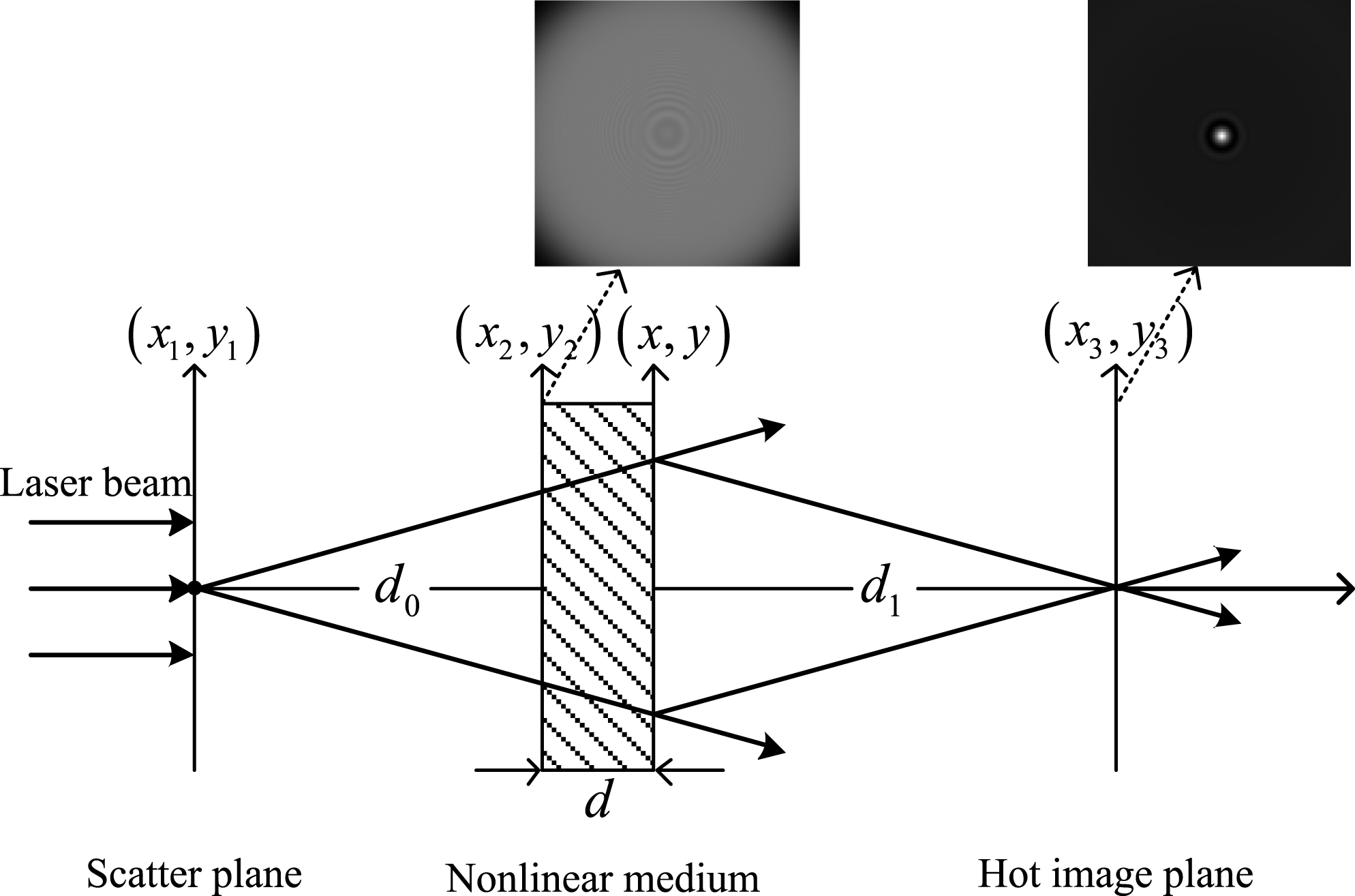
Figure 1. Schematic diagram of the hot-image formation process.
The field is composed of two parts: the background wave
 $U_{R}=A\exp (\text{i}kd_{0})$
and the weak perturbation
$U_{R}=A\exp (\text{i}kd_{0})$
and the weak perturbation
 $U_{0}$
. As damage size is only about tens of microns, amplitude of
$U_{0}$
. As damage size is only about tens of microns, amplitude of
 $U_{0}$
is much weaker than that of
$U_{0}$
is much weaker than that of
 $U_{R}$
, i.e.,
$U_{R}$
, i.e.,
 $|U_{0}|\ll |U_{R}|$
. Intensity distribution of the field on the front surface appears as a weak oscillation. What is more, thickness
$|U_{0}|\ll |U_{R}|$
. Intensity distribution of the field on the front surface appears as a weak oscillation. What is more, thickness
 $d$
of the nonlinear plate is only about 3–5 cm. It shows that the induced diffraction effect in the plate can be ignored for the final analysis of the hot image. The weak intensity oscillation of the diffraction ring introduces a nonlinear phase on the rear surface. It is proportional to the intensity oscillation
$d$
of the nonlinear plate is only about 3–5 cm. It shows that the induced diffraction effect in the plate can be ignored for the final analysis of the hot image. The weak intensity oscillation of the diffraction ring introduces a nonlinear phase on the rear surface. It is proportional to the intensity oscillation
 $M$
, which is given as
$M$
, which is given as
 $$\begin{eqnarray}M=\frac{|U(x_{2},y_{2})|^{2}}{|U_{R}|^{2}}.\end{eqnarray}$$
That is to say, the nonlinear plate mainly induces a nonlinear phase-only modulation to the diffraction field
 $U(x_{2},y_{2})$
, which is written as
$U(x_{2},y_{2})$
, which is written as
 $$\begin{eqnarray}\displaystyle U(x,y) & = & \displaystyle U(x_{2},y_{2})\cdot \exp \left[\text{i}B\cdot \frac{|U(x_{2},y_{2})|^{2}}{|U_{R}|^{2}}\right]\nonumber\\ \displaystyle & = & \displaystyle U(x_{2},y_{2})\cdot \exp (\text{i}B\cdot M).\end{eqnarray}$$
 $B$
is the phase delay induced by the nonlinear plate and background intensity. It reflects the severity of self-focusing and can be treated as a known quantity. Formula (4) shows that the nonlinear phase distribution on the rear surface appears like a phase hologram. It almost totally determines the final distribution of the hot image. Therefore, it is reasonable to approximate
$B$
is the phase delay induced by the nonlinear plate and background intensity. It reflects the severity of self-focusing and can be treated as a known quantity. Formula (4) shows that the nonlinear phase distribution on the rear surface appears like a phase hologram. It almost totally determines the final distribution of the hot image. Therefore, it is reasonable to approximate
 $U(x_{2},y_{2})$
with
$U(x_{2},y_{2})$
with
 $U_{R}$
and
$U_{R}$
and
 $U(x,y)$
can be rewritten as
$U(x,y)$
can be rewritten as
 $$\begin{eqnarray}U(x,y)\approx U_{R}\cdot \exp (\text{i}B\cdot M).\end{eqnarray}$$
Finally, the nonlinear phase on the rear surface induces a focus point on the hot-image plane
 $(x_{3},y_{3})$
after another propagation distance
$(x_{3},y_{3})$
after another propagation distance
 $d_{1}$
(
$d_{1}$
(
 $d_{1}=d_{0}$
) in free space. Field of
$d_{1}=d_{0}$
) in free space. Field of
 $U(x_{3},y_{3})$
is given as
$U(x_{3},y_{3})$
is given as
 $$\begin{eqnarray}\displaystyle U(x_{3},y_{3}) & = & \displaystyle \frac{A}{\text{i}\unicode[STIX]{x1D706}d_{1}}\exp (\text{i}kd_{1})\displaystyle \iint \exp (\text{i}B\cdot M)\exp \left\{\frac{\text{i}k}{2d_{1}}\right.\nonumber\\ \displaystyle & & \displaystyle \times \left.[(x_{3}-x_{2})^{2}+(y_{3}-y_{2})^{2}]\vphantom{\frac{\text{i}k}{2d_{1}}}\right\}\,\text{d}x_{2}\,\text{d}y_{2}.\end{eqnarray}$$
It means that the defect and the hot image are located symmetrically about the nonlinear plate. Formulas (5) and (6) show that the hot image can be precisely calculated with the intensity oscillation
 $M$
of the diffraction ring.
$M$
of the diffraction ring.
Numerical simulation is conducted to verify the approximation in formulas (5) and (6). As super Gaussian beams are widely used in high power laser systems for the uniform irradiation in the inertial confinement fusion, a 10th-order super Gaussian beam with wavelength
 $\unicode[STIX]{x1D706}=1.053~\unicode[STIX]{x03BC}\text{m}$
in vacuum is set as the incident beam for example. Other properties of the beam are set as follows: waist radius
$\unicode[STIX]{x1D706}=1.053~\unicode[STIX]{x03BC}\text{m}$
in vacuum is set as the incident beam for example. Other properties of the beam are set as follows: waist radius
 $r_{w}=0.8~\text{cm}$
, fluence
$r_{w}=0.8~\text{cm}$
, fluence
 $\unicode[STIX]{x1D70C}=3.5~\text{J}/\text{cm}^{2}$
and pulse duration
$\unicode[STIX]{x1D70C}=3.5~\text{J}/\text{cm}^{2}$
and pulse duration
 $t=1~\text{ ns}$
. Area of the beam’s cross-section is
$t=1~\text{ ns}$
. Area of the beam’s cross-section is
 $2.048~\text{cm}\times 2.048~\text{cm}$
, which is divided into
$2.048~\text{cm}\times 2.048~\text{cm}$
, which is divided into
 $1024\times 1024$
grid points. Parameters of the plate are set as follows: the refractive index
$1024\times 1024$
grid points. Parameters of the plate are set as follows: the refractive index
 $n_{0}=1.528$
, the nonlinear refractive coefficient
$n_{0}=1.528$
, the nonlinear refractive coefficient
 $\unicode[STIX]{x1D6FE}=3.1\times 10^{-16}~\text{cm}^{2}/\text{W}$
, and the thickness
$\unicode[STIX]{x1D6FE}=3.1\times 10^{-16}~\text{cm}^{2}/\text{W}$
, and the thickness
 $d=5~\text{cm}$
. Propagation distance in free space is set as
$d=5~\text{cm}$
. Propagation distance in free space is set as
 $d_{1}=d_{0}=50~\text{cm}$
. Two identical defects are used to scatter the incident light so that the symmetry between defects and hot images can be shown clearly. Amplitude modulation coefficient is 0.5. Phase modulation coefficient is
$d_{1}=d_{0}=50~\text{cm}$
. Two identical defects are used to scatter the incident light so that the symmetry between defects and hot images can be shown clearly. Amplitude modulation coefficient is 0.5. Phase modulation coefficient is
 $0.6\unicode[STIX]{x1D70B}$
. The damage radius is
$0.6\unicode[STIX]{x1D70B}$
. The damage radius is
 $50~\unicode[STIX]{x03BC}\text{m}$
. Interval between the two defects is
$50~\unicode[STIX]{x03BC}\text{m}$
. Interval between the two defects is
 $200~\unicode[STIX]{x03BC}\text{m}$
. In order to verify the approximation, fields on the rear surface are respectively expressed as the nonlinear phase multiplied with the background field and the diffraction field on the front surface. The simulative results are named as Estimation and Original.
$200~\unicode[STIX]{x03BC}\text{m}$
. In order to verify the approximation, fields on the rear surface are respectively expressed as the nonlinear phase multiplied with the background field and the diffraction field on the front surface. The simulative results are named as Estimation and Original.

Figure 2. Locations and peak intensities of hot images. (a) Two hot-image planes are both located at
 $Z=49~\text{cm}$
; (b) the extracted intensity distributions and lateral positions of hot images.
$Z=49~\text{cm}$
; (b) the extracted intensity distributions and lateral positions of hot images.
Figure 2(a) shows the peak intensities at each observation plane from the rear surface of the nonlinear plate (
 $Z$
denotes the distance between the rear surface and the observation plane). It indicates that two hot-image planes are both located at
$Z$
denotes the distance between the rear surface and the observation plane). It indicates that two hot-image planes are both located at
 $Z=49~\text{cm}$
. The location error of 1 cm is related with the thickness of the plate. Figure 2(b) shows the extracted intensity distributions and lateral positions of hot images on the hot-image plane. Peak intensity of the Estimation is
$Z=49~\text{cm}$
. The location error of 1 cm is related with the thickness of the plate. Figure 2(b) shows the extracted intensity distributions and lateral positions of hot images on the hot-image plane. Peak intensity of the Estimation is
 $4.766\times 10^{9}~\text{W}/\text{cm}^{2}$
. Peak intensity of the Original is
$4.766\times 10^{9}~\text{W}/\text{cm}^{2}$
. Peak intensity of the Original is
 $4.848\times 10^{9}~\text{W}/\text{cm}^{2}$
. The intensity error is just 1.69%, which can be ignored. The intervals between the peak intensities in Figure 2(b) are both equal to
$4.848\times 10^{9}~\text{W}/\text{cm}^{2}$
. The intensity error is just 1.69%, which can be ignored. The intervals between the peak intensities in Figure 2(b) are both equal to
 $200~\unicode[STIX]{x03BC}\text{m}$
, which shows that defects and hot images are symmetrically located about the nonlinear plate. Therefore, location and peak intensity of the hot image can be precisely calculated with the extracted intensity oscillation of the diffraction ring on the front surface of the nonlinear plate.
$200~\unicode[STIX]{x03BC}\text{m}$
, which shows that defects and hot images are symmetrically located about the nonlinear plate. Therefore, location and peak intensity of the hot image can be precisely calculated with the extracted intensity oscillation of the diffraction ring on the front surface of the nonlinear plate.
The background intensity is set prior to the full system operation. And the parameters such as
 $\unicode[STIX]{x1D706}$
,
$\unicode[STIX]{x1D706}$
,
 $\unicode[STIX]{x1D6FE}$
and
$\unicode[STIX]{x1D6FE}$
and
 $n_{0}$
are also known quantities. What is more, it is feasible to collect diffraction images in a series of low-energy shots prior to the high-energy shot. Therefore, adoption of the pure intensity information
$n_{0}$
are also known quantities. What is more, it is feasible to collect diffraction images in a series of low-energy shots prior to the high-energy shot. Therefore, adoption of the pure intensity information
 $M$
of the diffraction ring is a direct and efficient method to prejudge hot images, which is more practical than those conventional methods. Next step is to find an automatic and robust solution to detect these diffraction rings.
$M$
of the diffraction ring is a direct and efficient method to prejudge hot images, which is more practical than those conventional methods. Next step is to find an automatic and robust solution to detect these diffraction rings.
3 Detection of diffraction rings with the GDM method
3.1 Recognition of simulated diffraction rings
The GDM method is used to detect diffraction rings, which is known to be more robust than other phase matching methods[Reference Paglieroni and Eppler18–Reference Chen, Kegelmeyer, Liebman, Thaddeus Salmon, Tzeng and Paglieroni20]. A typical diffraction ring image is shown in Figure 3(a). It is obvious that a series of light and dark rings encircle a light spot. Its gradient direction field indicates the evolution of gray value, which is shown in Figure 4(a). One portion of the direction field points toward the center, whereas the other portion points outward from the center. This gradient direction field exhibits a perfect centrosymmetric distribution. Based on this feature, a luminance disk is chosen as the matching template, which is shown in Figure 3(b). Its gradient direction field is shown in Figure 4(b), which is extremely akin to the gradient direction field of a diffraction ring. All the gradient directions point toward the center.
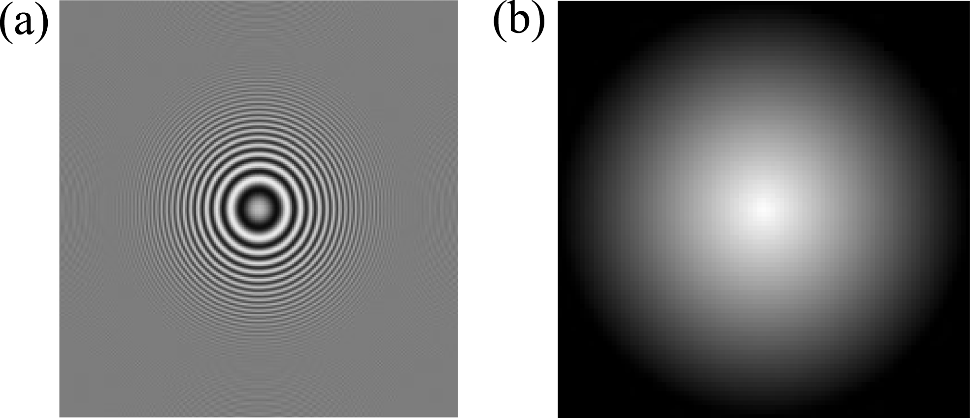
Figure 3. Evolution of gray value of the diffraction ring and the luminance disk. (a) Diffraction ring image; (b) luminance disk (matching template).
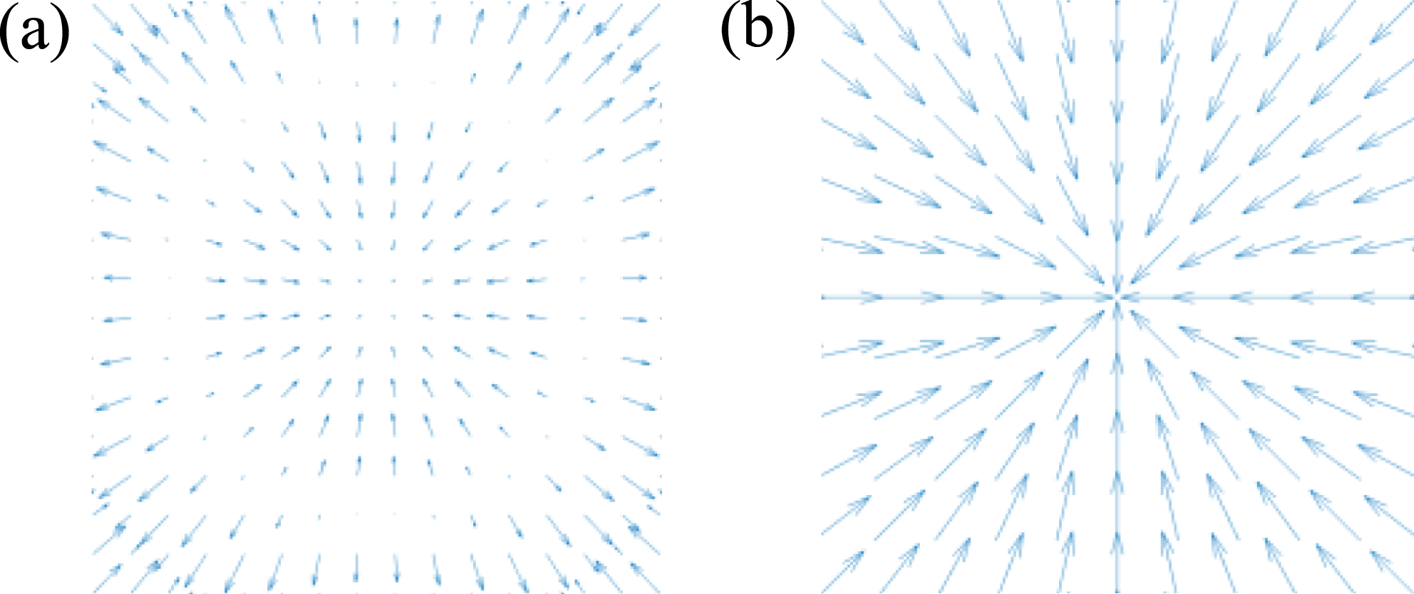
Figure 4. Gradient direction fields used to indicate the evolution of gray value. (a) Gradient direction field of the diffraction ring; (b) gradient direction field of the luminance disk.
Gradient direction matching is done to calculate the similarity distribution after the extraction of gradient direction fields. Cosine function is used to remove the influence of inversion between some parts of the two direction fields. Fast Fourier transform (FFT) is adopted to remove the limit of template size on the computational efficiency. Similarity threshold is set according to the above matching results. Center of the diffraction ring is finally found out, which corresponds to the local maxima in the similarity distribution. The entire algorithm flow is shown in Figure 5.
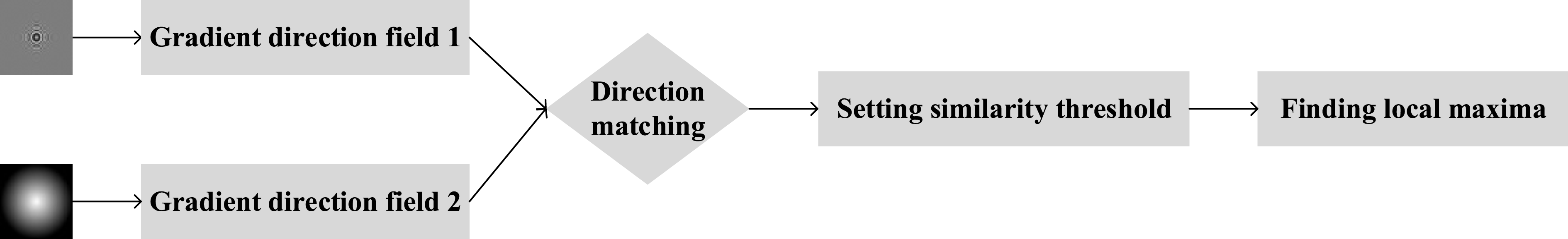
Figure 5. Flow chart of the GDM method.
In most cases, there may be multiple rings in the collected images, which are induced by multiple defects. Some of them are overlapped with different degrees. Multiple hot images will appear in just one high-energy shot under this condition, which is a serious threat to the system. Therefore, it is of great importance to study the performance of GDM to recognize overlapped diffraction rings. Research in the past years[Reference Yang, Liu, Gao, Miao and Zhu16, Reference Yang, Liu, Gao, Miao and Zhu17, Reference Chen, Kegelmeyer, Liebman, Thaddeus Salmon, Tzeng and Paglieroni20] has pointed out that only those diffraction rings with overlap ratio smaller than 50% can be recognized. Nevertheless, the experiments are conducted with actually collected images, and various noises would affect the above criterion. Therefore, a series of simulated diffraction rings are used to study the performance of this method, which are shown in Figure 6.
A plane wave with wavelength
 $\unicode[STIX]{x1D706}=632.8~\text{nm}$
in vacuum is set as the incident beam. Two identical simulated defects are selected to scatter the light with the radius
$\unicode[STIX]{x1D706}=632.8~\text{nm}$
in vacuum is set as the incident beam. Two identical simulated defects are selected to scatter the light with the radius
 $r_{s}=50~\unicode[STIX]{x03BC}\text{m}$
. Amplitude modulation coefficient is 0.8. Phase modulation coefficient is
$r_{s}=50~\unicode[STIX]{x03BC}\text{m}$
. Amplitude modulation coefficient is 0.8. Phase modulation coefficient is
 $0.6\unicode[STIX]{x1D70B}$
. Area of the beam’s cross-section is also
$0.6\unicode[STIX]{x1D70B}$
. Area of the beam’s cross-section is also
 $2.048~\text{cm}\times 2.048~\text{cm}$
, which is divided into
$2.048~\text{cm}\times 2.048~\text{cm}$
, which is divided into
 $1024\times 1024$
grid points. Diffraction distance in the simulation is 50 cm.
$1024\times 1024$
grid points. Diffraction distance in the simulation is 50 cm.
Figures 6(a)–6(d) represent the diffraction rings that are induced by two defects with intervals of 0.32 mm, 2.4 mm, 4.0 mm and 8.0 mm. The corresponding similarity distributions are respectively shown in Figures 6(e)–6(h). The detected centers of diffraction rings are labeled with red circles. Figures 6(c), 6(d), 6(g) and 6(h) show that the diffraction rings can be easily detected when the two rings are far apart from each other. Second, when the two defects are so close to each other that the induced rings interfere and form a regular light spot in the center, they can also be recognized. Figures 7(a) and 7(e) show an example of this situation. The inset in Figure 7(b) shows that the two rings are both seriously disturbed by the interference effect of them. Therefore, Figure 7(f) shows that they are not recognized.

Figure 6. Simulated diffraction rings and the recognition results. (a)–(d) Simulated diffraction rings with different overlap degrees; (e)–(h) similarity distributions and the detected centers.
In a word, the conventional criterion that the overlap ratio should be smaller than 50% is not enough. This result indicates that it is feasible to recognize diffraction rings with the GDM method as long as the regular structure of the central light spot in the diffraction ring is still reserved. Therefore, hot images induced by those closely spaced defects and the defects that are far apart from each other can be directly and automatically prejudged.
However, two kinds of random noises often appear in the actually collected images. One appears like salt & pepper noise, which does not break the regular structure of the central light spot in the diffraction ring but makes the conventional GDM method fail to recognize diffraction rings. Image compression is used to extract the inherent feature of intensity oscillation, which is applied before the extraction of the gradient direction field and is able to solve this problem. The other kind appears as some bright or dark spots near the center of the diffraction ring. It can induce some redundant centers that are very close to the real center, which will greatly limit the efficiency of automatic operation when a lot of images need to be processed in a short time. Cluster analysis based on the minimum distance is adopted to remove these adjacent centers.
3.2 Experimental research with the actually collected images
In order to verify the effect of image compression on optimizing the performance of the GDM method to process actually collected images, the spatial light modulator (SLM) is used to simulate a pure amplitude defect[Reference Dudley, Vasilyeu, Belyi, Khilo, Ropot and Forbes21]. Optical path is shown in Figure 7. The incident beam is a plane wave with wavelength
 $\unicode[STIX]{x1D706}=632.8~\text{nm}$
in vacuum.
$\unicode[STIX]{x1D706}=632.8~\text{nm}$
in vacuum.
 $\text{P}_{1}$
is the polarizer, which is used to make the polarization direction be parallel with the long side of SLM.
$\text{P}_{1}$
is the polarizer, which is used to make the polarization direction be parallel with the long side of SLM.
 $\text{P}_{2}$
is the attenuator. BS is the beam splitter. CCD is the charge-coupled device. Diffraction images are collected at different distances.
$\text{P}_{2}$
is the attenuator. BS is the beam splitter. CCD is the charge-coupled device. Diffraction images are collected at different distances.
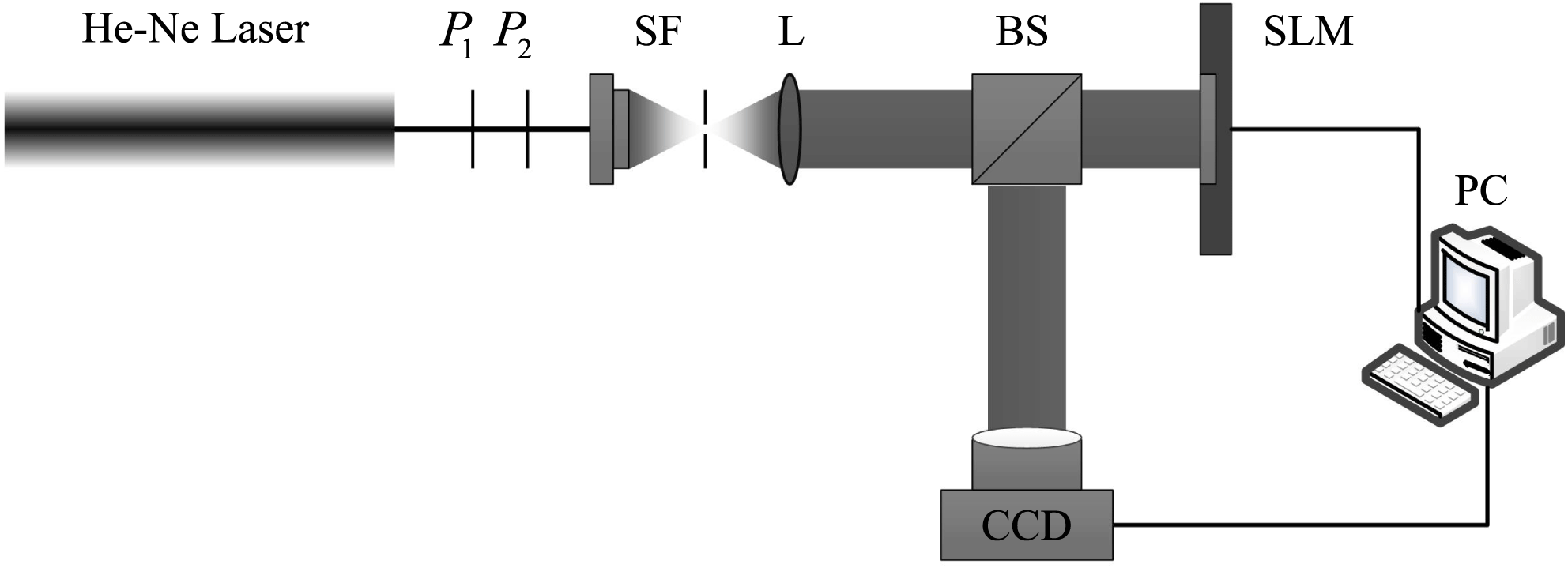
Figure 7. Experimental setup for the diffraction optical path that uses SLM to simulate a defect.
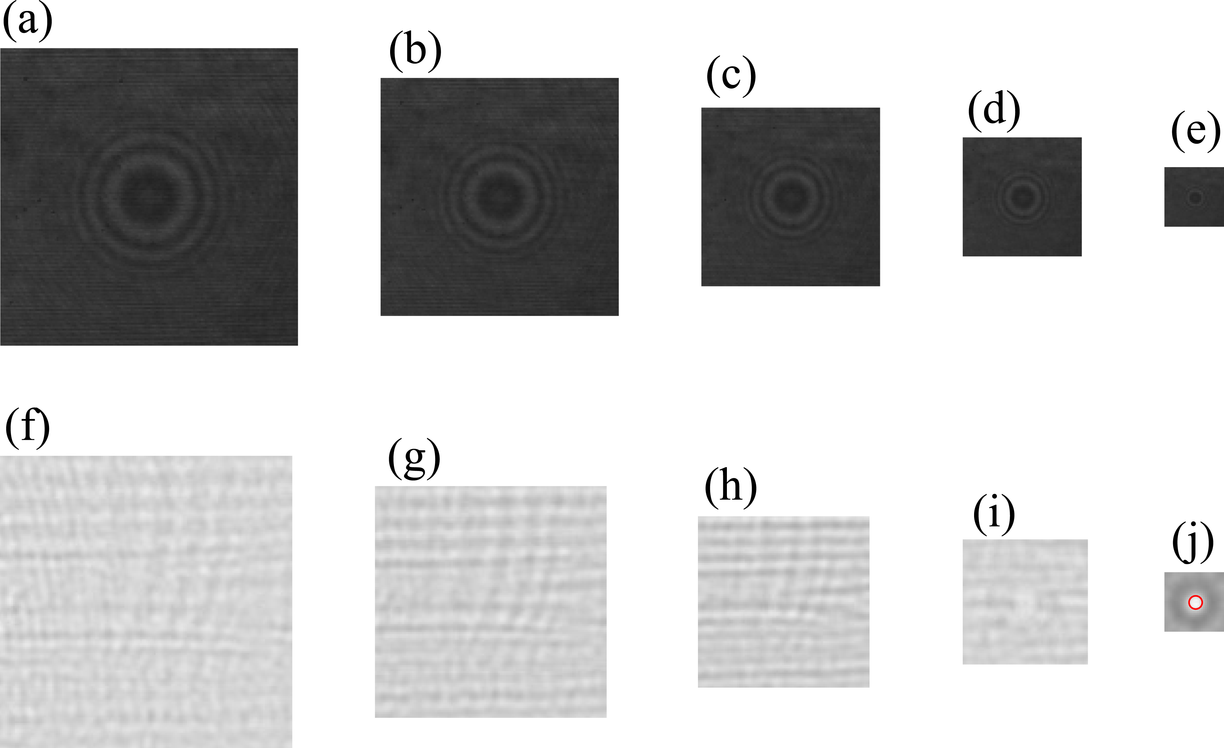
Figure 8. Diffraction ring images and similarity distributions. (a)–(e) Diffraction ring images with different compression ratios; (f)–(j) similarity distributions and the detected diffraction center labeled with a red circle.
Figure 8 shows one of the diffraction images collected at 30 cm, which is induced by a simulated defect with radius
 $r=80~\unicode[STIX]{x03BC}\text{m}$
. Image size is
$r=80~\unicode[STIX]{x03BC}\text{m}$
. Image size is
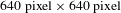 $640~\text{pixel}\times 640~\text{pixel}$
. Size of the matching template is
$640~\text{pixel}\times 640~\text{pixel}$
. Size of the matching template is
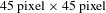 $45~\text{pixel}\times 45~\text{pixel}$
. It is clearly shown that this image is seriously disturbed by the first kind of noise. Therefore, this image is compressed with different ratios: 1.0, 0.8, 0.6, 0.4 and 0.2, which are shown respectively in Figures 8(a)–8(e). Similarity distributions are shown in Figures 8(f)–8(j). Results show that the diffraction center is finally recognized when the compression ratio is 0.2. The corresponding similarity matrix is
$45~\text{pixel}\times 45~\text{pixel}$
. It is clearly shown that this image is seriously disturbed by the first kind of noise. Therefore, this image is compressed with different ratios: 1.0, 0.8, 0.6, 0.4 and 0.2, which are shown respectively in Figures 8(a)–8(e). Similarity distributions are shown in Figures 8(f)–8(j). Results show that the diffraction center is finally recognized when the compression ratio is 0.2. The corresponding similarity matrix is
 $84\times 84$
in size.
$84\times 84$
in size.
In order to verify the effect of cluster analysis on optimizing the practicability of the GDM method in processing a lot of images in a short time automatically, a damaged plate is used to induce a series of seriously disturbed diffraction images. The plane wave used in the above experiment is still utilized to irradiate the plate. Figure 9(a) shows the diffraction ring image collected at 41 cm. The image is seriously affected by both the two kinds of random noises. Therefore, it is first compressed with ratio of 0.2. Size of the compressed image is
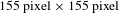 $155~\text{pixel}\times 155~\text{pixel}$
. Size of the matching template is
$155~\text{pixel}\times 155~\text{pixel}$
. Size of the matching template is
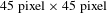 $45~\text{pixel}\times 45~\text{pixel}$
. Both similarity matrices are
$45~\text{pixel}\times 45~\text{pixel}$
. Both similarity matrices are
 $111\times 111$
in size. Figure 9(b) shows that six centers are initially detected, whose coordinates are labeled in the figure. Every three of them are closely spaced near one real center. Cluster analysis based on the minimum distance is adopted to classify these six centers and only two of them are left for the automatic operation, which is shown in Figure 9(c).
$111\times 111$
in size. Figure 9(b) shows that six centers are initially detected, whose coordinates are labeled in the figure. Every three of them are closely spaced near one real center. Cluster analysis based on the minimum distance is adopted to classify these six centers and only two of them are left for the automatic operation, which is shown in Figure 9(c).
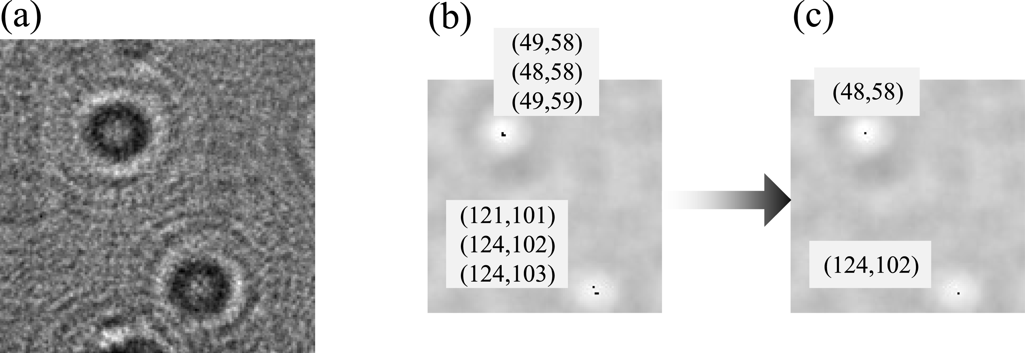
Figure 9. Diffraction ring image and similarity distributions. (a) The collected diffraction ring image at 41 cm; (b) similarity distribution with six initially detected centers; (c) similarity distribution with two centers left after cluster analysis.
In a word, the optimized GDM method with image compression and cluster analysis performs well in the actually collected images. It can recognize the diffraction rings that are induced by the defects of tens of microns and provide information for the automatic operation without any redundant messages. Therefore, hot images induced by defects of tens of microns can be directly prejudged.
4 Conclusion
In conclusion, analysis of hot-image formation process shows that the distribution of the hot image can be precisely calculated with the intensity oscillation of the diffraction ring on the front surface of the nonlinear plate. Based on this relationship, a direct prejudgement technique is put forward, which aims to automatically detect diffraction rings. Analysis of recognizing simulated diffraction rings shows that hot images induced by those closely spaced defects and the defects that are far apart from each other can be directly prejudged. The GDM method is optimized with the image compression and cluster analysis to recognize the diffraction rings in the actually collected images. Experimental results show that hot images induced by defects of tens of microns can be directly prejudged without redundant information. As this method can prejudge hot images with the pure intensity information of the diffraction ring, it is more practical than those conventional methods. Next research goal is to further identify those diffraction rings that are currently not recognized.
Acknowledgements
This work was supported by the International Partnership Program of Chinese Academy Of Sciences (No. 181231KYSB20170022), the National Natural Science Foundation of China (No. 11774364), and the Shanghai Sailing Program (No. 18YF1425900).


 Open access