


1. Introduction
The alignment system of a high power laser facility is used for deviation adjustment of beams. For an already running facility, the error caused by the vibrations will be magnified through beam transmitting and lead to beam deviation[Reference Liu, Liu, Zheng, Huang and Zhu1]. The alignment process mainly depends on the CCD real-time optical image analysis and processing; in general, these images contain a lot of noise. The noise mainly include (1) noise caused by electromagnetic interference, (2) noise caused by effects of stray light, (3) Gaussian noise that is generated by the internal resistive components, and (4) salt and pepper noise that is generated by image cutting or the photoelectric conversion process[Reference Mendoza2, Reference Faraji and MacLean3]. When the noise is serious, it not only affects spot identification and segmentation but also affects the calculation of center coordinates. The common approach is to remove this noise by an average filter or median filter, and then to use the threshold method to calculate the center of the spot for beam auto-alignment. A median filter can smooth the noise point but will cause image blur, while a median filter can avoid image blur, but will lose image detail such as corner and line information[Reference Bose4, Reference Gupta and Shandilya5].
In this paper, an improved multiple filter method for image denoising is proposed to replace traditional single filter methods. These multiple filters are constituted of an average filter and a median filter in different connection sequences, so that all advantages of both filters can be combined. Then, an adaptive step feedback adjustment mechanism is built to improve the alignment quality and processing time.
2. Multiple filter denoising
For the average filter algorithm, also called the neighborhood linear average method, the basic idea is use the average gray value of several neighboring pixels instead of the gray value of each pixel. The neighborhood is usually constituted of four or eight pixels that are around one pixel, as shown in Figure 1. An average filter is a kind of linear filter, using the smoothing feature of a linear filter to restrain the Gaussian noise and impulse noise. However, it will also cause a spot image in which especially the edges become blurred.
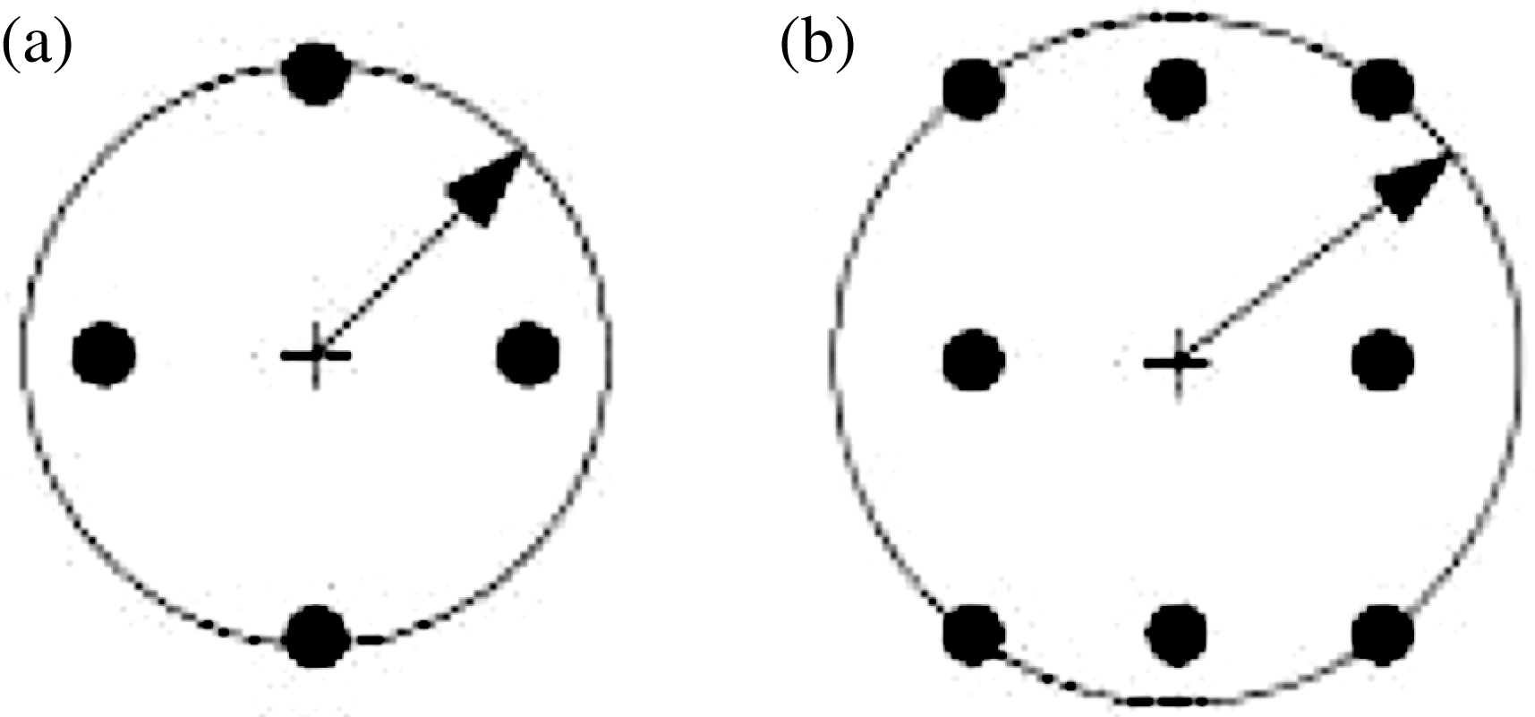
Figure 1. The neighborhood of an average filter; the point ‘ $\def \xmlpi #1{}\def \mathsfbi #1{\boldsymbol {\mathsf {#1}}}\let \le =\leqslant \let \leq =\leqslant \let \ge =\geqslant \let \geq =\geqslant \def \Pr {\mathit {Pr}}\def \Fr {\mathit {Fr}}\def \Rey {\mathit {Re}}+$’ is the selected pixel. (a) The neighborhood is constituted of four pixels; this is the simplest mode. (b) The neighborhood is constituted of eight pixels; the precision will be better than with four pixels.
For a given image, we can use a two-dimensional function  $f(x,y)$ to describe all pixels of this image. For a pixel point $(x,y)$, supposing that the neighborhood is $r\ast r$ ( $r$ is even), the output of the average filter $\overline{f} (x,y)$ is calculated by
 $$\begin{equation} \label {eq1} \overline f (x,y)=\frac {1}{r\ast r} \sum _{i=-\frac {r}{2}}^{\frac {r}{2}} \sum _{j=-\frac {r}{2}}^{\frac {r}{2}} f(x+i,y+j) . \end{equation}$$
The basic idea of a median filter is to sort all gray values of each pixel in one neighborhood first, and then to use the middle position gray value instead of the gray value of the center pixel of the neighborhood. The neighborhood is usually constituted of nine or 25 pixels that are around one pixel, as shown in Figure 2. Because salt and pepper noise often appears in the form of isolated points, and each point is constituted by only a few pixels, a median filter is effective in restraining salt and pepper noise and has almost no influence on the image edges. However, for large noise, and especially for Gaussian noise, the restraining ability of a median filter is weaker than that of an average filter.
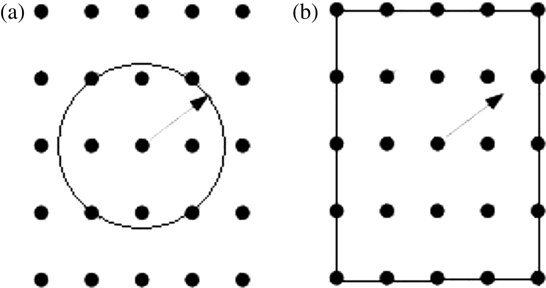
Figure 2. The neighborhood of a median filter; the center point is the selected pixel. (a) The neighborhood is constituted of nine pixels; this is the most commonly used mode. (b) The neighborhood is constituted of 25 pixels; the precision will be better than for the mode with nine pixels but requires more processing time.
For a given image, a two-dimensional function  $f(x,y)$ can describe all pixels. For a pixel point $(x,y)$, supposing that the neighborhood is $a\ast a$ ( $a$ is odd), so that there are $n=a\ast a$ gray values $\{ a_{1} ,a_{2} ,\ldots, a_{n} \} $ in this neighborhood, the value in the middle position will output as the selected pixel gray value after sorting, so the output of the median filter $\overline{f} (x,y)$ can be expressed by
 $$\begin{equation} \label {eq2} \overline f (x,y)={\rm med} \{ a_{1} ,a_{2} ,\ldots , a_{n} \}. \end{equation}$$
In order to combine the advantages of these filters, multiple filters are built to perform the image processing; these multiple filters are constituted of an average filter and a median filter in different connection sequencess. According to the sequence of connection, there are two types of multiple filter, the median–linear filter and the linear–median filter.
For the median–linear filter, referred to as ML, the output is calculated by
 $$\begin{equation} \label {eq3} \overline f (x,y)=\frac {1}{r\ast r} \sum _{i=-\frac {r}{2}}^{\frac {r}{2}} \sum _{j=-\frac {r}{2}}^{\frac {r}{2}} {\rm med}(f(x+i,y+j)). \end{equation}$$
For the linear–median filter, referred to as LM, the output is calculated by
 $$\begin{equation} \label {eq4} \overline f (x,y)={\rm med}\left (\frac {1}{r\ast r} \sum _{i=-\frac {r}{2}}^{\frac {r}{2}} \sum _{j=-\frac {r}{2}}^{\frac {r}{2}} (f(x+i,y+j))\right ). \end{equation}$$
For the median–linear filter, median filtering will be performed first. This procedure can remove the salt and pepper noise without losing image data. It also has the ability to weaken the effect of Gaussian noise. Then the average filter is used to filter most of Gaussian noise. Since the median filtering has the ability to distinguish the edge, the boundary of the spot image and the noise will have a significantly improved result. Under these circumstances, if the spot area of the image is large enough and the gray values of the spot and the noise have an obvious difference, then the effect of blurring that is produced by the median filter can be ignored.
If the noise is in the form of isolated points appearing in the image and rarely affects multiple pixels, and the gray values of the spot and the noise are closer, then the linear–median filter will be better.

Figure 3. Original images of the near and far fields. (a), (b) Near-field images. (c), (d) Far-field images.

Figure 4. Images of threshold processing without a filter. (a), (b) Near-field images. (c), (d) Far-field images.
After the performance of image denoising, the threshold gravity method[Reference Davies6, Reference Liu and Kuang7] is normally used to calculate the spot center position. This method usually sets a threshold value and then converts the images into two-dimensional value images. During this process, if the size of some image is  $A*B$, $f(i ,j)$ is the gray value of one pixel and the gray threshold value is set as $T$, then the threshold procedure can be expressed as
 $$\begin{equation} \label {eq5} F(x,y)=\left \{ \begin{array}{@{}ll} f(x,y), & f(x,y)\ge T, \\ 0, & f(x,y)\le T. \end{array} \right . \end{equation}$$
 When the center of gravity method is used to calculate centrality, a binarized matrix is actually calculated to obtain the center coordinates  $(x_{0} ,y_{0} )$, as follows:
 $$\begin{eqnarray} x_{o} =\frac {\sum _{x=1}^A \sum _{y=1}^B F(x,y)x} {\sum _{x=1}^A \sum _{y=1}^B F(x,y)}, \nonumber \\ y_{o} =\frac {\sum _{x=1}^A \sum _{y=1}^B F(x,y)y} {\sum _{x=1}^A \sum _{y=1}^B F(x,y)}. \label {eq6} \end{eqnarray}$$
The original beam images that are captured by digital CCDs are shown in Figure 3. Figures 3(a) and (b) are near-field images. From these images we can see that the near field has a clear image and a larger spot; Gaussian white noise is the main noise. Therefore, the main purpose of the near-field image is to remove Gaussian white noise, so the median–linear filter is appropriate for this situation. Figures 3(c) and (d) are far-field images. For these images, the imaging is not clear and the spot area is smaller than for the near-field ones. The main noise is salt and pepper noise, so the linear–median filter is better here.
If we directly perform threshold processing on these images without denoising, the results are shown in Figure 4. Gaussian noise is very obvious in Figures 4(a) and (b); salt and pepper noise is very obvious in Figures 4(c) and (d). The presence of these types of noise will have a serious effect on the calculation of the center.
For the near-field images, using the median–linear filter to denoise first and then performing the threshold processing, the detailed procedure is as follows:
(i) execute median filtering to remove salt and pepper noise;
(ii) execute average filtering to weaken Gaussian noise;
(iii) execute threshold processing and obtain the gray-scale map;
(iv) obtain the spot center by Equation (6) and calculate the deviation from the reference position;
(v) adjust the mirrors through the motor feedback control system.
The results of processing the image are shown in Figure 5.
The detailed procedure for the far field is similar to the above steps; the only difference is that the average filtering is performed first, and then the median filter is used to remove salt and pepper noise as well as to restore the clarity of the images. The results are shown in Figure 6.

Figure 5. Near-field images after multiple filters. (a), (e) The original images captured by near-field CCD. (b), (f) After use of a median–linear filter with 25 pixels. (c), (g) After use of an average filter with eight pixels. (d), (h) The images after threshold processing has been performed.
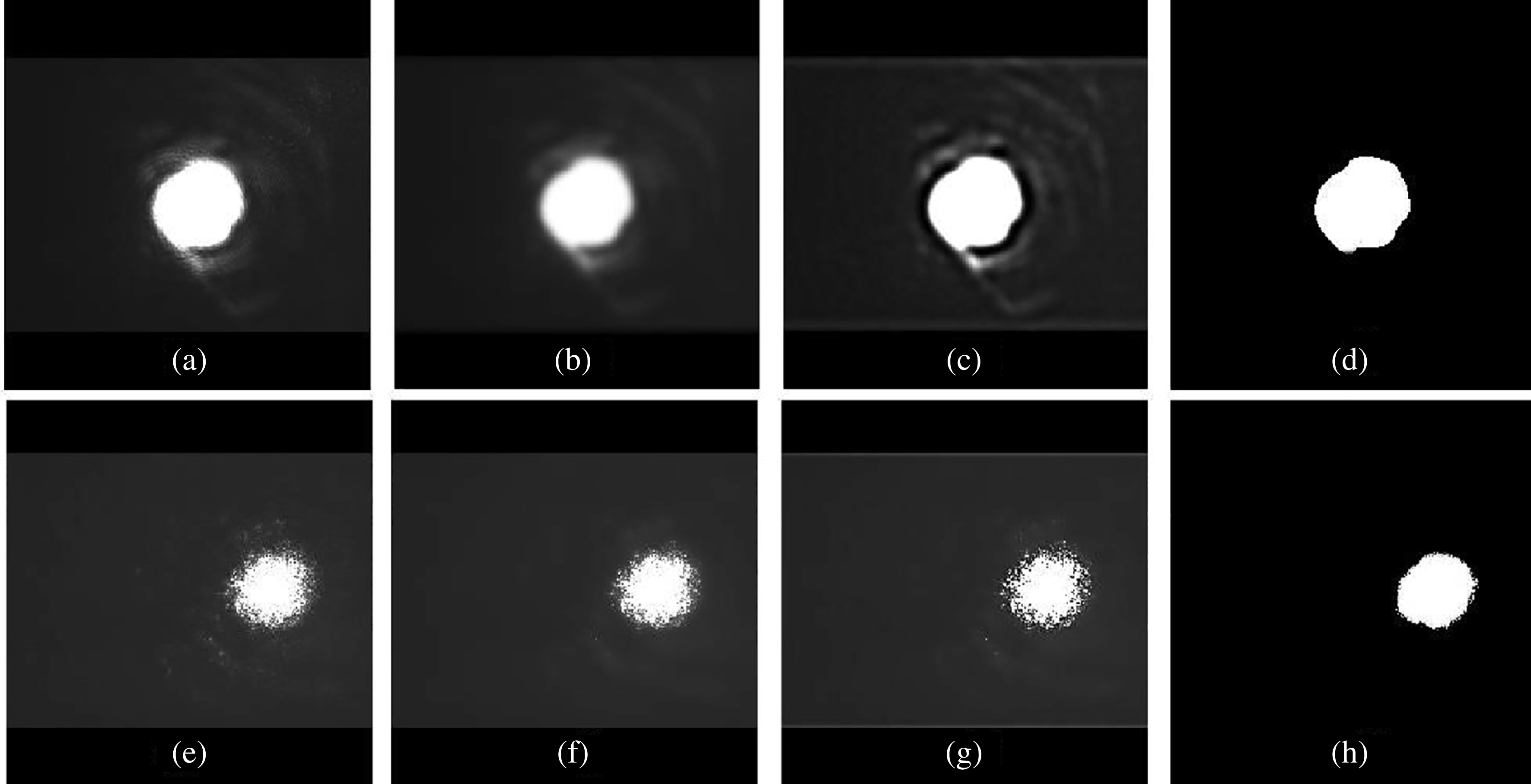
Figure 6. Far-field images after multiple filters. (a), (e) The original images captured by far-field CCD. (b), (f) After use of an average filter with eight pixels. (c), (g) After use of a median–linear filter with 25 pixels. (d), (h) The images after threshold processing has been performed.
3. Motor feedback control
The processed image captured by digital CCD is used to calculate the deviation, and the feedback control is used to align the beam path, which is accomplished by converting the deviation into motor rotation steps. The image center calculation and motor rotation are key factors, which directly affect the reflector adjustment. To finish the alignment in the shortest time, parallel alignment is conducted in the multi-path laser system. Therefore, the speed of image processing for a single path determines the alignment efficiency of the whole system[Reference Lv, Liu, Xu, Cao and Fan8, Reference Liu, Ding and Gao9].
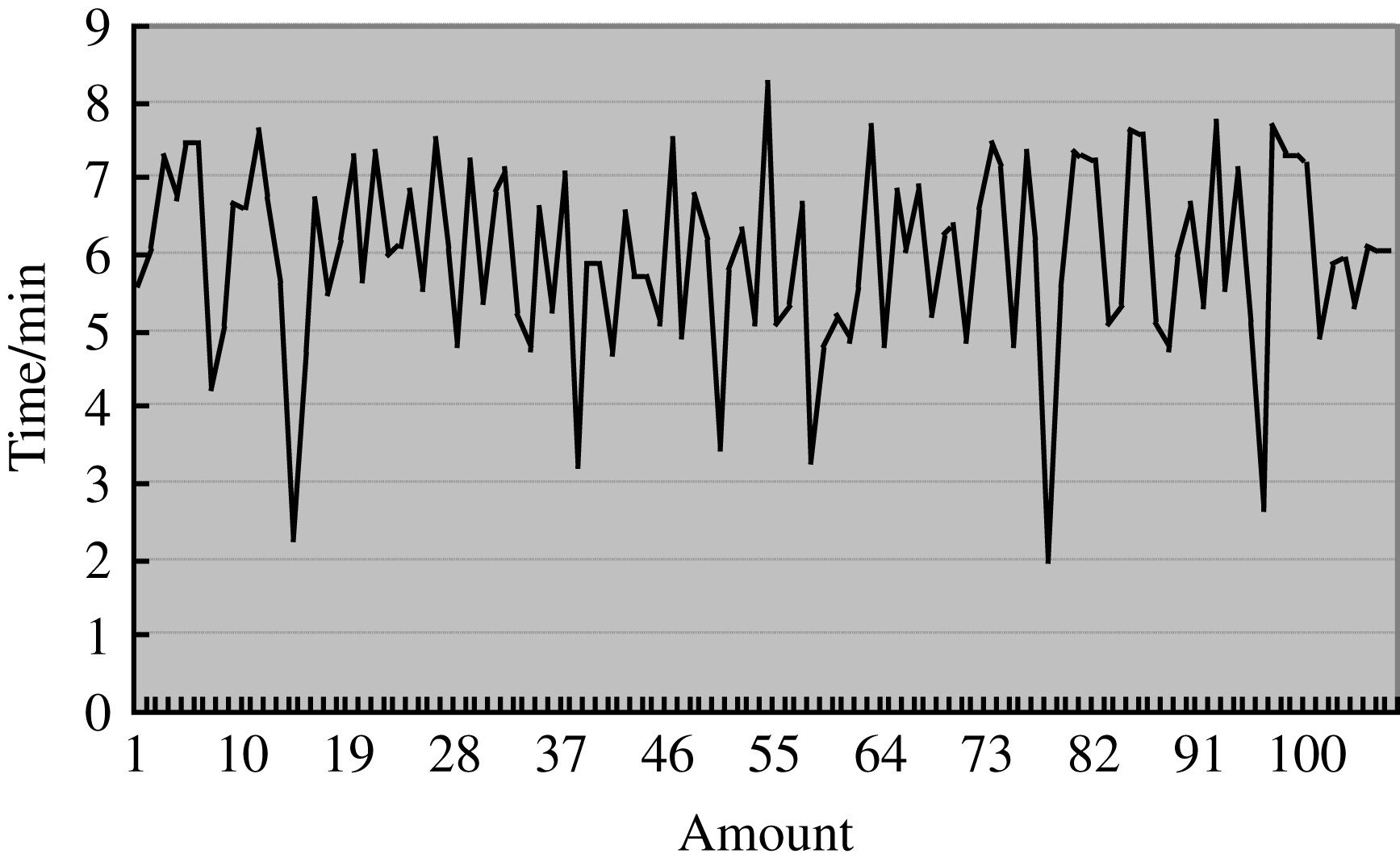
Figure 7. The results of the iteration method without a filter.
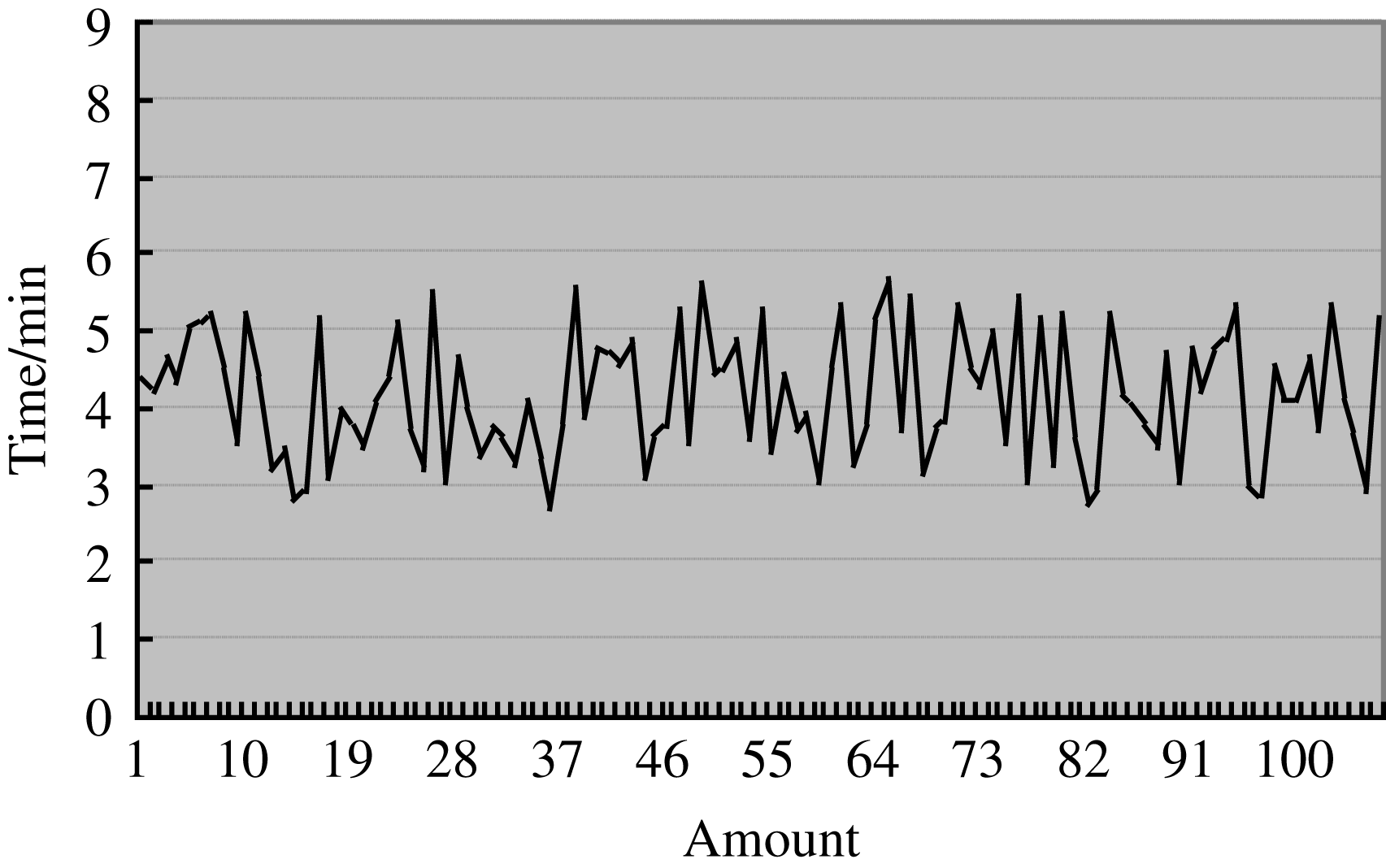
Figure 8. The result of the adaptive variable step method with filter denoising.
Ideally, the motor rotation step number is a fixed value corresponding to a pixel, according to the step number; it is only necessary to align once to adjust the beam center back to the reference position. However, as it is affected by interference factors, the relation between the pixel and the motor rotation step number is nonlinear in real time. The alignment feedback adjustment procedure adopts multiple iterations to adjust the beam path until the deviation of the beam center position is acceptable. The number of iterations is a random function of the pixel and the motor step number, which theoretically depends on the goodness of the fit between the random function and the nonlinear relationship. Therefore, the adjustment time fluctuates violently.
In order to eliminate the influence of the nonlinear relation between the pixel and the motor rotation step number, and moreover to reduce the number of iterations of mirror adjustment, we introduce a fuzzy control algorithm to rapidly align the beam with the specified center. The fuzzy control algorithm can realize universal approximation performance of the unknown control structure and obtain an adaptive variable related to the pixel and motor rotation step number. In other words, the real-time adaptive variable step control is determined by the actual deviation distance, which is determined by a fuzzy decision in accordance with the fuzzy rule. This ensures the fast and accurate automatic alignment, and enhances the robustness of the system [Reference Lee10, Reference Kovacic and Bogdan11].
First, fuzzy linguistic rules are used to change the experience and knowledge of the facility into fuzzy control rules. Because this process does not depend on an accurate mathematical model of the controlled object, we can ignore the effect of non-linear quantitative distance adjustment when the deviation is large. The real-time adaptive variable step will reduce when the spot center approaches the reference position; when it is close to the reference position, the adaptive variable step will become small. The adaptive variable step value is determined by the specific evaluation function and is quantified by fuzzy rules.
The fuzzy control uses a two-dimensional fuzzy controller. The deviation  $e$ and the deviation change $e_c$ are inputs, their corresponding linguistic variables are set as $E$ and $E_C$, the output is the control quantity $u$ and the corresponding linguistic variable is set as $U$.
$U$.
The linguistic variable value set of  $E_C$ and $U$ can be expressed as
 $$\begin{equation} \label {eq7} E_C=U=\{\mathit {NB},\mathit {NM},\mathit {NS},O,\mathit {PS},PM,PB\}. \end{equation}$$
The corresponding meanings are negative-big/negative-medium/negative-small/zero/positive-small/positive-medium/positive-big/.
The linguistic variable value set of  $E$ can be expressed as
 $$\begin{equation} \label {eq8} E =\{\mathit {NB}, \mathit {NM}, \mathit {NS}, \mathit {NO}, \mathit {PO}, \mathit {PS}, \mathit {PM}, \mathit {PB}\}. \end{equation}$$
The corresponding meanings are negative-big/negative-medium/negative-small/negative-zero/positive-zero/positive-small/positive-medium/positive-big.
The fuzzy rule of  $e$ and $e_{c}$ is
 $$\begin{eqnarray} E=\left \{ \begin{array}{@{}ll} 0, & e\le 2; \\ \mathit {INT}(e/25), & 2<e. \end{array} \right .\nonumber \\ E_{c} =\left \{ \begin{array}{@{}ll} 0, & e_{c} \le 2; \\ \mathit {INT}(e_{c} /20), & 2<e_{c} . \end{array} \right . \label {eq9} \end{eqnarray}$$
The conditional statement of the fuzzy control rules is
 $$\begin{eqnarray} &&\mbox {if } E=A_{i} \quad \mbox {then}\quad \mbox {if} \quad E_{c} =B_{j} \quad \mbox {then } U=C_{ij}\nonumber \\ &&\quad (i=1,2,\ldots ,8;j=1,2,\ldots ,7\}.\label {eq10} \end{eqnarray}$$
 The  $A_{i}$, $B_{j}$, and $C_{ij} $ respectively belong to deviation set $E$, deviation change $E_C$, and control quantity set
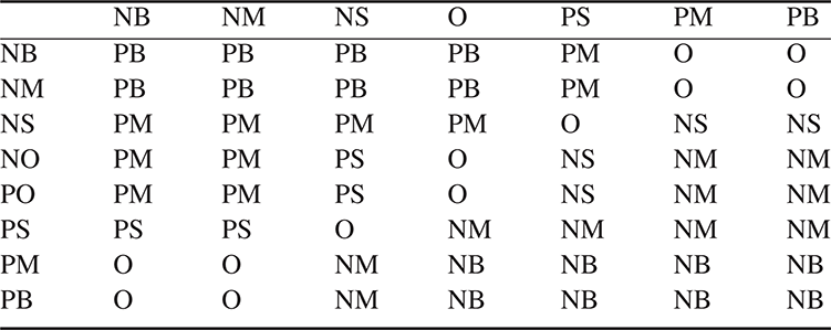
  $U$. Equation (10) can also be expressed as Table 1.
Table 1. Fuzzy control rule.
When the alignment is begun, CCDs will capture beam images for processing to obtain the deviation  $e$ and the amount of deviation change $e_c$. Then, according to Equations (7) and (8) we can get the values of $E$ and $E_C$; thus, the output of the control quantity $U$ can be obtained from Equation (10) by inquiry, Table 1; the value of $U$ determines the variable step size and number of rotation steps. The above procedures should be repeated until the center of the beam reaches the specified location.
4. Experimental results
In order to verify the validity of the image processing and fuzzy control in this paper, the following experiment is conducted. A small simulation platform is built in accordance with the SG II ninth beam path, which is driven by a motor to move 14 reflectors. The platform is monitored by seven sets of optical imaging systems composed of CCDs and optical lenses. In the experiment, the reflectors in a path are moved by some random steps to deflect the beam center. Then, the beam path is adjusted to make the beam center return to the reference position. The experiment is repeated 100 times, and the corresponding alignment times are recorded to be plotted as shown in Figures 7 and 8.
Figure 7 is the time curve of the original scheme. The original scheme first calculates the center error by a center of gravity method for the threshold value, and then adjusts the beam to the path center by multiple iterations. Figure 8 is the time curve of the new scheme. The new scheme first calculates the center error after filtering by the hybrid filter. Then, the optical path is adjusted by an adaptive variable step method. It can be seen that the time consumed and stability of the new scheme have a very significant improvement. The reflector adjustment process is completed in less than 4 min and the overall time for the system is less than 5 min.
In these 100 experiments, the fastest image processing time is 9 s (in SF1 far-field CCD) and the slowest image processing time is 57 s (in SF7 near-field CCD); the main processing time distribution is 27–46 s. The far-field image processing time is faster than the near-field image processing time. Because the image is processed three times, the time cost is increased, but the fuzzy control can effectively reduce the amount of iteration adjustment and save time. By using the fuzzy control, the adjustment can be finished in 3–5 steps and the accuracy is up to  $\pm $1 pixel; the old scheme needs 6–10 adjustment steps and the accuracy is only up to $\pm $1 pixel.
5. Conclusion
This method provides improved image processing of a laser alignment system based on mean filtering and median filtering, which is combined with the operating characteristics of a large amount of Gaussian noise and impulse noise in the imaging process of the laser alignment system. The correction speed of the path center and the computational accuracy are improved by different hybrid filters in accordance with the near- and far-field spot features. In addition, an adaptive step feedback adjustment mechanism based on a fuzzy algorithm is built to lower the impact of the nonlinear random relation between the unit pixel and motor adjustment steps. It improves the fast automatic alignment capability and the robustness of the system.
Acknowledgements
This paper was supported by grants from the Chinese and Israeli cooperation project on high power laser technology (2010DFB70490).


 Open access