


1 Introduction
Shock waves are some of the most interesting and prevalent phenomena in astrophysics. They are ubiquitous throughout the universe and their role in the transport of energy into the interstellar medium is fundamental[Reference Zel’dovich and Raizer1]. Hence, the understanding of the structure of the interstellar medium requires knowledge of the dynamics and evolution of shock waves[Reference McKee and Draine2]. Radiative shocks occur when shocked matter becomes hot enough that radiative transport modifies the shock structure and its dynamics[Reference Shull and McKee3]. In some low density cases, the heated post-shock medium is ionized and emits radiation which leads to radiative cooling. Radiation from the post-shock region can also heat and ionize the unshocked medium ahead of the shock giving rise to a radiative precursor. Radiative shocks are observed in accretion shocks[Reference Commerçon, Audit, Chabrier and Chièze4], supernova remnants[Reference Blondin, Wright, Borkowski and Reynolds5], bow shocks at the head of stellar jets[Reference Raga, Mellema, Arthur, Binette, Ferruit and Steffen6] and pulsating stars[Reference Huguet and Lafon7]. Moreover, radiative shocks are also predicted to exhibit thermal cooling instabilities[Reference Hunter8], which occur due to an imbalance between heating and cooling rates, which is a topic of high interest in astrophysics since they could be related to the formation of several astrophysical objects, for example star formation[Reference McKee and Draine2]. For these reasons, the study of radiative shocks is a research area of great interest at present.
The possibility of scaling the magnetohydrodynamics equations between astrophysics and laboratory flows[Reference Ryutov, Drake, Kane, Liang, Remington and Wood-Vasey9–Reference Bouquet, Falize, Michaut, Gregory, Loupias, Vinci and Koenig13] and the development of high-energy density (HED) facilities[Reference Remington, Drake and Ryutov14], such as high-power lasers and fast magnetic pinch generators, have allowed the design of HED laboratory astrophysics experiments. High-power lasers have been commonly used to perform experiments to produce radiative shocks in gases with different approaches: irradiating a pin or a foil within a moderate to high Z background gas[Reference Edens, Ditmire, Hansen, Edwards, Adams, Rambo, Ruggles, Smith and Porter15–Reference Edens, Adams, Rambo, Ruggles, Smith, Porter and Ditmire17], directly depositing the laser energy into clustered gases[Reference Keilty, Liang, Ditmire, Remington, Shigemori and Rubenchick18–Reference Symes, Hohenberger, Doyle, Smith, Moore, Gumbrell, Rodriguez and Gil20] or driving a solid piston into a gas cell or tube[Reference Bouquet, Stéhle, Koenig, Chieze, Benuzzi-Mounaix, Batani, Leygnac, Fleury, Merdji, Michaut, Thais, Grandjouan, Hall, Henry, Malka and Lafon21–Reference Chaulagain, Stehle, Larour, Kozlova, Suzuki-Vidal, Barroso, Cotelo, Velarde, Rodriguez, Gil, Ciardi, Acef, Nejdl, de Sa, Singh, Ibgui and Champion25].
New experiments have been recently performed to investigate the collision and interaction of two counter-propagating piston-driven radiative shocks[Reference Rodriguez, Espinosa, Gil, Florido, Rubiano, Mendoza, Martel, Minguez, Symes, Hohenberger and Smith26–Reference Singh, Stehlé, Suzuki-Vidal, Kozlova, Larour, Chaulagain, Clayson, Rodriguez, Gil, Nejdl, Krus, Dostal, Dudzak, Barroso, Acef, Cotelo and Velarde29] and their radiative precursors. These experiments open new applications in the area of laboratory astrophysics, such as the study of reflected and transmitted radiative shock and the interaction of a radiative shock with a denser medium in astrophysics scenarios, and were conducted at the Prague Asterix Laser System (PALS)[Reference Jungwirth, Cejnarova, Juha, Kralikova, Krasa, Krousky, Krupickova, Laska, Masek, Mocek, Pfeifer, Prag, Renner, Rohlena, Rus, Skala, Straka and Ullschmied30] and Orion high-power laser[Reference Hopps, Oades, Andrew, Brown, Cooper, Danson, Daykin, Duffield, Edwards, Egan, Elsmere, Gales, Girling, Gumbrell, Harvey, Hillier, Hoarty, Horsfield, James, Leatherland, Masoero, Meadowcroft, Norman, Parker, Rothman, Rubery, Treadwell, Winter and Bett31] facilities. The macroscopic properties of the experiment were simulated with NYM[Reference Roberts, Rose, Thomson and Wright32] and PETRA[Reference Youngs33] radiation-hydrodynamics codes. On the other hand, either for the radiation-hydrodynamics simulations or to interpret experimental data, such as the absorption or emission spectra, plasma microscopic properties, such as the composition and radiative properties of the plasma, must be obtained and analyzed since they provide useful and complementary information to radiation-hydrodynamics simulations.
The main objective of this work is to provide a description of microscopic properties of the plasmas generated in the experiments described above. We have therefore performed numerical simulations of the atomic and radiative properties of the post-shock and radiative precursor regions of radiative shocks in xenon. For this purpose, the plasma conditions (mass densities and electron temperatures) used in the microscopic simulations were provided by the radiation-hydrodynamics (rad-hydro) simulations performed with the NYM and PETRA codes. In particular, we have studied the thermodynamic regime of the plasma in both the post-shock and radiative precursor regions, the monochromatic opacities and emissivities, and the charge state distributions (CSDs) for times prior to the shocks collision as after this time the xenon mixes with the piston material (plastic and bromine). An analysis of the specific intensities of the radiation emitted by the plasma of both regions at early times was made, when the interaction between the shocks and the radiative precursors is weak and the spectra are due to a single shock. However, some of the results obtained could also be useful in analyzing the spectra at later times when the radiative precursors interact. The analysis of the intensities may also be helpful for future experiments in assessing whether an experimental capability (such as emission spectroscopy) would be useful. Finally, the radiation-hydrodynamics simulations predicted hydrodynamic instabilities that could be due to the strong cooling of the radiative shocks. For this reason, a theoretical analysis of the possibility of the onset of thermal instabilities in these experiments has been carried out.
This paper is structured as follows. Section 2 is devoted to presenting the theoretical model used in the computation of the microscopic properties. In Section 3, a brief description of the experimental setup and the radiation-hydrodynamics simulations are shown. Section 4 presents the results of the simulations of the radiative and spectroscopic properties of the post-shock and the radiative precursor regions together with the analysis of the thermal instabilities in the cooling layer in the post-shock medium. Finally, conclusions are drawn in Section 5.
2 Theoretical model
The calculation of plasma radiative and spectroscopic properties requires the use of atomic data, such as energy levels, oscillator strengths, cross-sections and atomic-level populations. The following section briefly describes the models used in this work to calculate these values.
2.1 Atomic data
The oscillator strengths, energy levels and photoionization cross-sections were calculated using FAC code[Reference Gu34], in which a fully relativistic approach based on the Dirac equation was used. The photoionization cross-sections were obtained in the context of the relativistic distorted wave approximation. In this work, the atomic data were calculated by the relativistic detailed configuration accounting (RDCA) approach. The unresolved transition array (UTA)[Reference Bauche, Bauche-Arnoult and Klapisch35] formalism was used for the bound–bound transitions. Therefore, the transition energies include the UTA shift and the width of each transition is considered for the line profile. Furthermore, a correction to the oscillator strengths due to the configuration interaction within the same nonrelativistic configurations was included.
The selection of the atomic configurations for population kinetics simulations is a key factor but still an open question, overall for complex elements like xenon with a large number of electrons. In this work, we have included configurations with energies up to three times the ionization potential. This choice should be adequate for accurate modeling of thermal plasmas[Reference Peyrusse, Bauche-Arnoult and Bauche36, Reference Hansen, Bauche, Bauche-Arnoult and Gu37].
According to this criterion, the following configurations were included: (1) ground configuration; (2) single excited configuration from the valence shell,
 $n_{v}$
, to shells with
$n_{v}$
, to shells with
 $n\leqslant 10$
; (3) doubly excited configurations from the valence shell to shells with
$n\leqslant 10$
; (3) doubly excited configurations from the valence shell to shells with
 $n\leqslant n_{v}+2$
; and (4) single excited configurations from shell
$n\leqslant n_{v}+2$
; and (4) single excited configurations from shell
 $n_{v}-1$
to shells with
$n_{v}-1$
to shells with
 $n\leqslant n_{v}+2$
.
$n\leqslant n_{v}+2$
.
2.2 Determination of plasma atomic-level populations
For high densities, when the plasma reaches local thermodynamic equilibrium (LTE), the population of the ionization stages,
 $N_{\unicode[STIX]{x1D701}}$
, is obtained from the Saha equation given by
$N_{\unicode[STIX]{x1D701}}$
, is obtained from the Saha equation given by
 $$\begin{eqnarray}\displaystyle \frac{N_{\unicode[STIX]{x1D701}+1}n_{e}}{N_{\unicode[STIX]{x1D701}}}=\frac{Z_{\unicode[STIX]{x1D701}+1}Z_{e}}{Z_{\unicode[STIX]{x1D701}}}e^{-(I_{\unicode[STIX]{x1D701}-}\unicode[STIX]{x0394}I_{\unicode[STIX]{x1D701}})/kT_{e}}, & & \displaystyle\end{eqnarray}$$
where
 $Z_{\unicode[STIX]{x1D701}}$
and
$Z_{\unicode[STIX]{x1D701}}$
and
 $Z_{e}$
are the partition functions of ion
$Z_{e}$
are the partition functions of ion
 $\unicode[STIX]{x1D701}$
and free electrons, respectively,
$\unicode[STIX]{x1D701}$
and free electrons, respectively,
 $n_{e}$
is the free electron density,
$n_{e}$
is the free electron density,
 $I_{\unicode[STIX]{x1D701}}$
is the ionization potential and
$I_{\unicode[STIX]{x1D701}}$
is the ionization potential and
 $\unicode[STIX]{x0394}I_{\unicode[STIX]{x1D701}}$
denotes the continuum lowering (CL) which models the depression of the ionization potential due to the plasma environment. In this work, we have applied the formulation due to Stewart and Pyatt[Reference Stewart and Pyatt38]. Once the ion populations were obtained through the Saha equation, the populations of the atomic levels for each ionization stage could then be obtained using the Boltzmann distribution function.
$\unicode[STIX]{x0394}I_{\unicode[STIX]{x1D701}}$
denotes the continuum lowering (CL) which models the depression of the ionization potential due to the plasma environment. In this work, we have applied the formulation due to Stewart and Pyatt[Reference Stewart and Pyatt38]. Once the ion populations were obtained through the Saha equation, the populations of the atomic levels for each ionization stage could then be obtained using the Boltzmann distribution function.
For arbitrary densities, the atomic-level populations can be determined from the solution of a system of collisional-radiative (CR) rate equations. This set of kinetic equations is given by
 $$\begin{eqnarray}\displaystyle \frac{\text{d}N_{\unicode[STIX]{x1D701}i}(\mathbf{r},t)}{\text{d}t} & = & \displaystyle \mathop{\sum }_{\unicode[STIX]{x1D701}^{\prime }j}N_{\unicode[STIX]{x1D701}^{\prime }j}(\mathbf{r},t)\mathbb{R}_{\unicode[STIX]{x1D701}^{\prime }j\rightarrow \unicode[STIX]{x1D701}i}^{+}\nonumber\\ \displaystyle & & \displaystyle -\,\mathop{\sum }_{\unicode[STIX]{x1D701}^{\prime }j}N_{\unicode[STIX]{x1D701}i}(\mathbf{r},t)\mathbb{R}_{\unicode[STIX]{x1D701}i\rightarrow \unicode[STIX]{x1D701}^{\prime }j}^{-},\end{eqnarray}$$
where
 $N_{\unicode[STIX]{x1D701}i}$
is the population density of the atomic level
$N_{\unicode[STIX]{x1D701}i}$
is the population density of the atomic level
 $i$
of the ion with charge state
$i$
of the ion with charge state
 $\unicode[STIX]{x1D701}$
. The terms
$\unicode[STIX]{x1D701}$
. The terms
 $\mathbb{R}_{\unicode[STIX]{x1D701}^{\prime }j\rightarrow \unicode[STIX]{x1D701}i}^{+}$
and
$\mathbb{R}_{\unicode[STIX]{x1D701}^{\prime }j\rightarrow \unicode[STIX]{x1D701}i}^{+}$
and
 $\mathbb{R}_{\unicode[STIX]{x1D701}i\rightarrow \unicode[STIX]{x1D701}^{\prime }j}^{-}$
take into account all the collisional and radiative processes which contribute to populate and depopulate the level
$\mathbb{R}_{\unicode[STIX]{x1D701}i\rightarrow \unicode[STIX]{x1D701}^{\prime }j}^{-}$
take into account all the collisional and radiative processes which contribute to populate and depopulate the level
 $\unicode[STIX]{x1D701}i$
, respectively.
$\unicode[STIX]{x1D701}i$
, respectively.
The set of rates equations in the CR model is coupled to the radiative transfer equation
 $$\begin{eqnarray}\displaystyle \frac{1}{c}\frac{\unicode[STIX]{x2202}I(\mathbf{r},t,\unicode[STIX]{x1D708},\mathbf{e})}{\unicode[STIX]{x2202}t}+\mathbf{e}\boldsymbol{\cdot }\unicode[STIX]{x1D735}I(\mathbf{r},t,\unicode[STIX]{x1D708},\mathbf{e})\hspace{30.0pt} & & \displaystyle \nonumber\\ \displaystyle =-\unicode[STIX]{x1D705}(\mathbf{r},t,\unicode[STIX]{x1D708})I(\mathbf{r},t,\unicode[STIX]{x1D708},\mathbf{e})+j(\mathbf{r},t,\unicode[STIX]{x1D708}), & & \displaystyle\end{eqnarray}$$
where
 $I$
is the specific intensity,
$I$
is the specific intensity,
 $\unicode[STIX]{x1D708}$
the photon frequency and
$\unicode[STIX]{x1D708}$
the photon frequency and
 $\mathbf{e}$
a unitary vector in the direction of propagation. Equations (2) and (3) are coupled through the emissivity and the absorption coefficients (
$\mathbf{e}$
a unitary vector in the direction of propagation. Equations (2) and (3) are coupled through the emissivity and the absorption coefficients (
 $j(\mathbf{r},t,\unicode[STIX]{x1D708})$
and
$j(\mathbf{r},t,\unicode[STIX]{x1D708})$
and
 $\unicode[STIX]{x1D705}(\mathbf{r},t,\unicode[STIX]{x1D708})$
, respectively).
$\unicode[STIX]{x1D705}(\mathbf{r},t,\unicode[STIX]{x1D708})$
, respectively).
The CR model as well as the Saha–Boltzmann (SB) equations used in this work is implemented in the MIXKIP code[Reference Espinosa, Rodriguez, Gil, Suzuki-Vidal, Lebedev, Ciardi, Rubiano and Martel39], a code developed to calculate plasma atomic-level populations of mono and multicomponent optically thin and thick plasmas in time-dependent and steady-state situations. The atomic processes included in the CR model implemented in MIXKIP are collisional ionization, three-body recombination, spontaneous decay, collisional excitation and deexcitation, radiative recombination, autoionization and electron capture. Furthermore, in order to take into account the effect of external radiation fields in the calculation of atomic-level populations, the radiative driven processes of photoexcitation, photodeexcitation and photoionization are included in the CR model. A more detailed description of the expressions used for the rates of the atomic processes can be found in Ref. [Reference Espinosa, Rodriguez, Gil, Suzuki-Vidal, Lebedev, Ciardi, Rubiano and Martel39]. Plasma self-absorption (i.e., opacity effects) is modeled in MIXKIP in an approximate way using the escape factor formalism for the bound–bound opacity[Reference Mancini, Joyce and Hooper40].
Once the rate or SB equations (Equations (1) and (2), respectively) are solved, both the plasma average ionization and the plasma CSD, defined as the set of the population densities of the ions present in the plasma for a given condition of density and temperature, can be obtained.
2.3 Calculation of radiative properties
To calculate the radiative properties, we have used the RAPCAL code[Reference Rodríguez, Florido, Gil, Rubiano, Martel and Mínguez41]. The monochromatic emissivity and opacity (
 $j(\unicode[STIX]{x1D708})$
and
$j(\unicode[STIX]{x1D708})$
and
 $\unicode[STIX]{x1D705}(\unicode[STIX]{x1D708})$
, respectively), include bound–bound, bound-free and free–free contributions. In this work, the complete redistribution hypothesis was assumed for the line profile in the bound–bound transitions. This includes natural, Doppler, UTA and electron impact[Reference Dimitrijevic and Konjevin42] broadenings. The line shape function is applied with Voigt profiles incorporating all of these broadenings. For the bound-free contribution, we used the photoionization cross-section calculated with the FAC code in the relativistic distorted wave approach. Finally, for the free–free contribution, the Kramers semi-classical expression for the inverse bremsstrahlung[Reference Kramers43] cross-section was used.
$\unicode[STIX]{x1D705}(\unicode[STIX]{x1D708})$
, respectively), include bound–bound, bound-free and free–free contributions. In this work, the complete redistribution hypothesis was assumed for the line profile in the bound–bound transitions. This includes natural, Doppler, UTA and electron impact[Reference Dimitrijevic and Konjevin42] broadenings. The line shape function is applied with Voigt profiles incorporating all of these broadenings. For the bound-free contribution, we used the photoionization cross-section calculated with the FAC code in the relativistic distorted wave approach. Finally, for the free–free contribution, the Kramers semi-classical expression for the inverse bremsstrahlung[Reference Kramers43] cross-section was used.
3 Description of the experimental setup and radiation-hydrodynamics simulations
The experiments[Reference Suzuki-Vidal, Clayson, Stehlé, Swadling, Foster, Skidmore, Graham, Burdiak, Lebedev, Chaulagain, Singh, Gumbrell, Patankar, Spindloe, Larour, Kozlova, Rodriguez, Gil, Espinosa, Velarde and Danson27] were conducted on the Orion laser and the setup consisted of gas cells filled with xenon at
 ${\sim}0.3$
bar
${\sim}0.3$
bar
 $({\sim}1.6\times 10^{-3}~\text{g}\cdot \text{cm}^{-3})$
. Plastic discs were attached to opposite octagonal faces, separated by 4 mm, which acted as pistons. Shocks were driven by focusing four laser beams (each beam
$({\sim}1.6\times 10^{-3}~\text{g}\cdot \text{cm}^{-3})$
. Plastic discs were attached to opposite octagonal faces, separated by 4 mm, which acted as pistons. Shocks were driven by focusing four laser beams (each beam
 ${\sim}400~\text{J}$
,
${\sim}400~\text{J}$
,
 $\unicode[STIX]{x03BB}=351~\text{nm}$
, 1 ns pulse duration) onto each piston (laser intensity
$\unicode[STIX]{x03BB}=351~\text{nm}$
, 1 ns pulse duration) onto each piston (laser intensity
 ${\sim}5\times 10^{14}~\text{W}/\text{cm}^{2}$
). These experiments were diagnosed with point projection X-ray backlighting (XRBL) and laser optical interferometry. XRBL provided information about the post-shock region. For the radiative precursor, laser interferometry was used to measure the free electron density along the probe beam path. The large xenon volume used in the experiments resulted in shocks with quasi-spherical geometry. A collision between the two shocks occurred after
${\sim}5\times 10^{14}~\text{W}/\text{cm}^{2}$
). These experiments were diagnosed with point projection X-ray backlighting (XRBL) and laser optical interferometry. XRBL provided information about the post-shock region. For the radiative precursor, laser interferometry was used to measure the free electron density along the probe beam path. The large xenon volume used in the experiments resulted in shocks with quasi-spherical geometry. A collision between the two shocks occurred after
 ${\sim}30~\text{ns}$
followed by the formation of reverse shocks. The XRBL images indicated a shock velocity of around
${\sim}30~\text{ns}$
followed by the formation of reverse shocks. The XRBL images indicated a shock velocity of around
 $75\pm 25~\text{km}/\text{s}$
and a reverse shock velocity of around 30 km/s. Figure 1 shows an example of results from rad-hydro simulations and experiments, with XRBL results, shown in Figure 1(c) at 25 ns.
$75\pm 25~\text{km}/\text{s}$
and a reverse shock velocity of around 30 km/s. Figure 1 shows an example of results from rad-hydro simulations and experiments, with XRBL results, shown in Figure 1(c) at 25 ns.
2D rad-hydro simulations were performed using then NYM and PETRA codes. NYM is a Lagrangian code with multigroup implicit Monte Carlo X-ray transport and full laser-interaction physics. This code was, therefore, used to model the laser–piston interaction. The simulations provided by the NYM code were linked to the Eulerian code PETRA which used multigroup X-ray diffusion to study the late time plasma behavior (after
 ${\sim}5~\text{ns}$
). The collision of the counter-propagating shocks was simulated assuming a fully reflective boundary (for hydrodynamics and radiation) at the center of the diagnostic window (at a distance of 2 mm from the position of the pistons) both for the plasma flow and for the radiation. In general, the simulations accurately reproduced the overall shock dynamics[Reference Youngs33]. As an example, Figures 1(a) and 1(b) show 2D maps of density of matter and electron temperatures of one of the shocks at 16 ns, obtained from the simulations. In Figure 2, we also show the axial profiles of the mass densities and electron temperatures for times analyzed in this work.
${\sim}5~\text{ns}$
). The collision of the counter-propagating shocks was simulated assuming a fully reflective boundary (for hydrodynamics and radiation) at the center of the diagnostic window (at a distance of 2 mm from the position of the pistons) both for the plasma flow and for the radiation. In general, the simulations accurately reproduced the overall shock dynamics[Reference Youngs33]. As an example, Figures 1(a) and 1(b) show 2D maps of density of matter and electron temperatures of one of the shocks at 16 ns, obtained from the simulations. In Figure 2, we also show the axial profiles of the mass densities and electron temperatures for times analyzed in this work.

Figure 1. (a) Simulated mass density and (b) simulated electron temperature at 16 ns. (c) Experimental X-ray backlighting at 25 ns. The dashed lines mark the position of the diagnostic window on the gas-cell targets.
4 Results
4.1 Analysis of the radiative precursor
Figure 3 shows the axial profiles of the electron temperatures and mass densities of one of the radiative shocks (propagating from left to right) at
 $8$
and 16 ns obtained from 2D rad-hydro simulations. For the latter, the profile of the electron densities is also presented. The shock front is located at the highest temperature and ahead of the shock front a radiative precursor is observed. Simulations suggest that temperatures in the radiative precursor range from
$8$
and 16 ns obtained from 2D rad-hydro simulations. For the latter, the profile of the electron densities is also presented. The shock front is located at the highest temperature and ahead of the shock front a radiative precursor is observed. Simulations suggest that temperatures in the radiative precursor range from
 $2$
to 20 eV at 8 ns. As time progresses, the lowest temperatures in the radiative precursor increase (maybe due to the proximity of the other shock and the overlapping of the two radiative precursors), as shown in Figure 3 right. At 8 ns the whole range of temperatures mentioned above is present. At this early time, we can consider the whole system as a single shock because the interaction between the two shocks is not predominant as the radiative precursors are not yet overlapping.
$2$
to 20 eV at 8 ns. As time progresses, the lowest temperatures in the radiative precursor increase (maybe due to the proximity of the other shock and the overlapping of the two radiative precursors), as shown in Figure 3 right. At 8 ns the whole range of temperatures mentioned above is present. At this early time, we can consider the whole system as a single shock because the interaction between the two shocks is not predominant as the radiative precursors are not yet overlapping.

Figure 2. Electron temperature (dashed lines) and mass density profiles of one of the radiative shocks as a function of time and position obtained with the 2D radiative-hydrodynamic simulation.

Figure 3. Axial electron temperature (orange) and mass density (blue) profiles of one of the radiative shocks at 8 ns and 16 ns, deduced from the 2D radiation-hydrodynamics simulations. An electron density profile is also represented in green at 16 ns.
Figure 3 shows that the characteristic time of the evolution of plasma conditions is of the order of
 ${\sim}\text{ns}$
. However, the characteristic time of the dominant atomic processes (electron–ion collisions) in the plasma,
${\sim}\text{ns}$
. However, the characteristic time of the dominant atomic processes (electron–ion collisions) in the plasma,
 $t_{a}$
, is given by[Reference Salzmann44]
$t_{a}$
, is given by[Reference Salzmann44]
 $$\begin{eqnarray}\displaystyle t_{a}=\frac{1}{n_{e}\langle \unicode[STIX]{x1D70E}v\rangle }, & & \displaystyle\end{eqnarray}$$
where
 $\unicode[STIX]{x1D70E}$
is the cross-section of the dominant process and
$\unicode[STIX]{x1D70E}$
is the cross-section of the dominant process and
 $v$
is the electron velocity. This yields time scales of around 1–100 fs for the plasma conditions under consideration, which is considerably lower than the characteristic time of the plasma evolution. Therefore, the atomic kinetics calculations can be performed assuming the plasma as in steady state, and thus the left-hand side in Equation (2) vanishes. Furthermore, simulations including plasma self-absorption (i.e., opacity effects) were carried out, obtaining that the effects in the calculation of the plasma level populations were not relevant. This implies that the rate and the radiative transfer equations (given in Equations (2) and (3), respectively) will be uncoupled. This result agrees with previous studies of blast waves experiments launched in xenon gas clusters conducted on the THOR laser system with similar ranges of plasma densities and temperatures[Reference Rodriguez, Espinosa, Gil, Florido, Rubiano, Mendoza, Martel, Minguez, Symes, Hohenberger and Smith26]. Finally, we have also analyzed the effect in the calculation of the plasma level populations of the radiative processes due to the radiation emitted by the shock. With that purpose, the specific intensity of the radiation emitted by the shock was simulated using a diluted Planckian function at the temperature of the front shock. This confirmed that the influence of the external radiation field, for a given plasma condition, was small and thus could be neglected. Therefore, according to these results, the atomic kinetic model employed in this work for the microscopic simulations was the collisional-radiative steady-state (CRSS) model (Equation (2) with the left-hand side equal to zero) without including the plasma radiation self-absorption and external radiation fields. In Figure 4, the CSDs of the xenon plasma for the range of temperatures of the radiative precursor and its mass density (
$v$
is the electron velocity. This yields time scales of around 1–100 fs for the plasma conditions under consideration, which is considerably lower than the characteristic time of the plasma evolution. Therefore, the atomic kinetics calculations can be performed assuming the plasma as in steady state, and thus the left-hand side in Equation (2) vanishes. Furthermore, simulations including plasma self-absorption (i.e., opacity effects) were carried out, obtaining that the effects in the calculation of the plasma level populations were not relevant. This implies that the rate and the radiative transfer equations (given in Equations (2) and (3), respectively) will be uncoupled. This result agrees with previous studies of blast waves experiments launched in xenon gas clusters conducted on the THOR laser system with similar ranges of plasma densities and temperatures[Reference Rodriguez, Espinosa, Gil, Florido, Rubiano, Mendoza, Martel, Minguez, Symes, Hohenberger and Smith26]. Finally, we have also analyzed the effect in the calculation of the plasma level populations of the radiative processes due to the radiation emitted by the shock. With that purpose, the specific intensity of the radiation emitted by the shock was simulated using a diluted Planckian function at the temperature of the front shock. This confirmed that the influence of the external radiation field, for a given plasma condition, was small and thus could be neglected. Therefore, according to these results, the atomic kinetic model employed in this work for the microscopic simulations was the collisional-radiative steady-state (CRSS) model (Equation (2) with the left-hand side equal to zero) without including the plasma radiation self-absorption and external radiation fields. In Figure 4, the CSDs of the xenon plasma for the range of temperatures of the radiative precursor and its mass density (
 ${\sim}1.6\times 10^{-3}~\text{g}\cdot \text{cm}^{-3}$
) are displayed. The figure shows that the ions present in the range of temperatures of the radiative precursor span from
${\sim}1.6\times 10^{-3}~\text{g}\cdot \text{cm}^{-3}$
) are displayed. The figure shows that the ions present in the range of temperatures of the radiative precursor span from
 $\text{Xe}^{0+}$
to
$\text{Xe}^{0+}$
to
 $\text{Xe}^{10+}$
, and that, as the charge state increases, the presence of these more charged ions in the plasma spreads over a large range of temperature, due to the increase of the ionization potential. Thus, for example, at 4 eV the abundance of
$\text{Xe}^{10+}$
, and that, as the charge state increases, the presence of these more charged ions in the plasma spreads over a large range of temperature, due to the increase of the ionization potential. Thus, for example, at 4 eV the abundance of
 $\text{Xe}^{0+}$
is already negligible but, on the other hand, the abundance of
$\text{Xe}^{0+}$
is already negligible but, on the other hand, the abundance of
 $\text{Xe}^{7+}$
ion (atomic structure
$\text{Xe}^{7+}$
ion (atomic structure
 $5s^{1}$
), is noticeable from 7 eV to temperatures higher than 18 eV.
$5s^{1}$
), is noticeable from 7 eV to temperatures higher than 18 eV.

Figure 4. Charge state distribution (CSD) as a function of the electron temperature at the mass density in the radiative precursor (
 $1.6\,\times$
 $10^{-3}~\text{g}\cdot \text{cm}^{-3}$
).
$10^{-3}~\text{g}\cdot \text{cm}^{-3}$
).
The CSDs were also calculated assuming LTE, that is, through the SB equations (Equation (1)), obtaining very small differences in the average ionization between LTE and NLTE calculations. These differences could be greater for the CSD since this is a less average quantity than the average ionization. However, the differences in the fractional abundances only begin to emerge for
 $\text{Xe}^{8+}$
ions at temperatures around 15 eV (although these differences are lower than 5%) and become more noticeable at 18 eV. At this temperature, the LTE model predicts that the most abundant ion is
$\text{Xe}^{8+}$
ions at temperatures around 15 eV (although these differences are lower than 5%) and become more noticeable at 18 eV. At this temperature, the LTE model predicts that the most abundant ion is
 $\text{Xe}^{9+}$
with an average ionization of
$\text{Xe}^{9+}$
with an average ionization of
 $8.70$
while the NLTE model predicts the most abundant ion as
$8.70$
while the NLTE model predicts the most abundant ion as
 $\text{Xe}^{8+}$
with an average ionization of
$\text{Xe}^{8+}$
with an average ionization of
 $8.50$
. Therefore, the LTE approach is accurate enough for the calculation of the average ionization and CSDs for temperatures lower than 18 eV, with slight differences at higher temperatures.
$8.50$
. Therefore, the LTE approach is accurate enough for the calculation of the average ionization and CSDs for temperatures lower than 18 eV, with slight differences at higher temperatures.
The range of electron densities obtained from the CRSS simulations in the radiative precursor varies from
 $4.08\times 10^{18}~\text{cm}^{-3}$
at 2 eV to
$4.08\times 10^{18}~\text{cm}^{-3}$
at 2 eV to
 $6.70\times 10^{19}~\text{cm}^{-3}$
at 20 eV, obtaining similar results to the ones provided by the radiation-hydrodynamics simulations, which use SESAME tables for the opacities and equations of state. For example, the electron densities obtained with the atomic kinetic model at
$6.70\times 10^{19}~\text{cm}^{-3}$
at 20 eV, obtaining similar results to the ones provided by the radiation-hydrodynamics simulations, which use SESAME tables for the opacities and equations of state. For example, the electron densities obtained with the atomic kinetic model at
 $4,12$
and 20 eV were
$4,12$
and 20 eV were
 $1.72\times 10^{19}$
,
$1.72\times 10^{19}$
,
 $4.77\times 10^{19}$
and
$4.77\times 10^{19}$
and
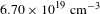 $6.70\times 10^{19}~\text{cm}^{-3}$
, respectively, whereas those obtained with the macroscopic simulation at 8 ns were
$6.70\times 10^{19}~\text{cm}^{-3}$
, respectively, whereas those obtained with the macroscopic simulation at 8 ns were
 $1.92\times 10^{19}$
,
$1.92\times 10^{19}$
,
 $4.63\times 10^{19}$
and
$4.63\times 10^{19}$
and
 $7.30\times 10^{19}~\text{cm}^{-3}$
, respectively, with relative differences lower than
$7.30\times 10^{19}~\text{cm}^{-3}$
, respectively, with relative differences lower than
 $10\%$
between both simulations. Since the temperatures used in the CRSS simulations are those provided by the rad-hydro simulations, the agreement between the electron densities obtained indicates that kinetic atomic models implemented in both simulations should provide similar values of the average ionization.
$10\%$
between both simulations. Since the temperatures used in the CRSS simulations are those provided by the rad-hydro simulations, the agreement between the electron densities obtained indicates that kinetic atomic models implemented in both simulations should provide similar values of the average ionization.
The electron densities of a region of the radiative precursor were experimentally obtained at 18 ns by means of laser interferometry[Reference Suzuki-Vidal, Clayson, Stehlé, Swadling, Foster, Skidmore, Graham, Burdiak, Lebedev, Chaulagain, Singh, Gumbrell, Patankar, Spindloe, Larour, Kozlova, Rodriguez, Gil, Espinosa, Velarde and Danson27]. The values obtained ranged from
 $1.85\times 10^{19}$
to
$1.85\times 10^{19}$
to
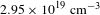 $2.95\times 10^{19}~\text{cm}^{-3}$
. As the mass density in the precursor does not change significantly from the initial density of the xenon gas fill, the average ionization can be determined. Using the mass density as an input, the CRSS model was used to determine the electron temperatures that provide similar average ionizations and electron densities to the experimental ones. This yielded temperatures from 4.20 to 6.50 eV for the radiative precursor. For that region of the radiative precursor, the hydrodynamic simulations predicted values of the electron densities from
$2.95\times 10^{19}~\text{cm}^{-3}$
. As the mass density in the precursor does not change significantly from the initial density of the xenon gas fill, the average ionization can be determined. Using the mass density as an input, the CRSS model was used to determine the electron temperatures that provide similar average ionizations and electron densities to the experimental ones. This yielded temperatures from 4.20 to 6.50 eV for the radiative precursor. For that region of the radiative precursor, the hydrodynamic simulations predicted values of the electron densities from
 $2.73\times 10^{19}$
to
$2.73\times 10^{19}$
to
 $3.10\times 10^{19}~\text{cm}^{-3}$
and electron temperatures from
$3.10\times 10^{19}~\text{cm}^{-3}$
and electron temperatures from
 $6.20$
to 7.17 eV. These 2D simulations slightly overestimate the values of the electron density with respect to the experimental ones and, therefore, the electron temperatures as well[Reference Suzuki-Vidal, Clayson, Stehlé, Swadling, Foster, Skidmore, Graham, Burdiak, Lebedev, Chaulagain, Singh, Gumbrell, Patankar, Spindloe, Larour, Kozlova, Rodriguez, Gil, Espinosa, Velarde and Danson27].
$6.20$
to 7.17 eV. These 2D simulations slightly overestimate the values of the electron density with respect to the experimental ones and, therefore, the electron temperatures as well[Reference Suzuki-Vidal, Clayson, Stehlé, Swadling, Foster, Skidmore, Graham, Burdiak, Lebedev, Chaulagain, Singh, Gumbrell, Patankar, Spindloe, Larour, Kozlova, Rodriguez, Gil, Espinosa, Velarde and Danson27].
Although the electron densities reached in the radiative precursor are not particularly high, the surrounding plasma, modeled by the inclusion of the CL in the population calculation, introduces some differences in the CSDs since the electron temperatures were also low. Thus, for example, at 12 eV, the most relevant ions obtained with the simulation including the CL were
 $\text{Xe}^{6+}-\text{Xe}^{8+}$
, whereas the ones obtained with the simulation for the isolated situation were
$\text{Xe}^{6+}-\text{Xe}^{8+}$
, whereas the ones obtained with the simulation for the isolated situation were
 $\text{Xe}^{5+}-\text{Xe}^{7+}$
. This could lead to noticeable changes in the calculation of the spectra. Therefore, the effect of the plasma surrounding must be considered in the atomic kinetic calculations for these ranges of electron temperatures and densities.
$\text{Xe}^{5+}-\text{Xe}^{7+}$
. This could lead to noticeable changes in the calculation of the spectra. Therefore, the effect of the plasma surrounding must be considered in the atomic kinetic calculations for these ranges of electron temperatures and densities.
In the experiments[Reference Suzuki-Vidal, Clayson, Stehlé, Swadling, Foster, Skidmore, Graham, Burdiak, Lebedev, Chaulagain, Singh, Gumbrell, Patankar, Spindloe, Larour, Kozlova, Rodriguez, Gil, Espinosa, Velarde and Danson27, Reference Clayson, Suzuki-Vidal, Lebedev, Swadling, Stehlé, Burdiak, Foster, Skidmore, Graham, Gumbrell, Patankar, Spindloe, Chaulagain, Kozlova, Larour, Singh, Rodriguez, Gil, Espinosa, Velarde and Danson28], optical and X-ray diagnostics were fielded to study the plasma in the transverse direction to the direction of propagation of the radiative shocks. Therefore, radiation emitted from either the shocked material or from the radiative precursor will have to pass through regions of the radiative precursor with different temperatures. This material can absorb some of that radiation, before reaching the detectors. For this reason, the monochromatic opacities of the radiative precursor were studied. The monochromatic opacities in the radiative precursor were calculated for four different characteristic temperatures (4, 10, 16 and 20 eV) and are presented in Figures 4(a) and 4(b).
Figure 4(a) shows that the opacities for temperatures of
 $4$
and 10 eV are quite different. Analysis of the CSDs (Figure 4) shows that at 4 eV there are predominantly four ion species in the plasma,
$4$
and 10 eV are quite different. Analysis of the CSDs (Figure 4) shows that at 4 eV there are predominantly four ion species in the plasma,
 $\text{Xe}^{1+}-\text{Xe}^{4+}$
. The CSD at 10 eV shows that the ions species in the plasma are
$\text{Xe}^{1+}-\text{Xe}^{4+}$
. The CSD at 10 eV shows that the ions species in the plasma are
 $\text{Xe}^{4+}-\text{Xe}^{8+}$
although the abundance of
$\text{Xe}^{4+}-\text{Xe}^{8+}$
although the abundance of
 $\text{Xe}^{4+}$
and
$\text{Xe}^{4+}$
and
 $\text{Xe}^{8+}$
ions are minor compared to the other ions. Therefore, none of the relevant ions at 4 eV are at 10 eV. This fact explains the significant differences between both spectra. The bound–bound contribution at 4 eV is practically contained in photon energies between 0–30 eV which are associated with single electron transitions from
$\text{Xe}^{8+}$
ions are minor compared to the other ions. Therefore, none of the relevant ions at 4 eV are at 10 eV. This fact explains the significant differences between both spectra. The bound–bound contribution at 4 eV is practically contained in photon energies between 0–30 eV which are associated with single electron transitions from
 $5s$
and
$5s$
and
 $5p$
subshells. For photons with higher energies the main contribution is bound-free. At a temperature of 10 eV an absorption structure in the photon energy range 0–30 eV is present and primarily due to electron transitions in the same shell
$5p$
subshells. For photons with higher energies the main contribution is bound-free. At a temperature of 10 eV an absorption structure in the photon energy range 0–30 eV is present and primarily due to electron transitions in the same shell
 $n=5$
of
$n=5$
of
 $\text{Xe}^{5+}-\text{Xe}^{7+}$
ions. Another two significant absorption features are present for a temperature of 10 eV. The first one located around a photon energy of 60 eV is primarily due to electron transitions from
$\text{Xe}^{5+}-\text{Xe}^{7+}$
ions. Another two significant absorption features are present for a temperature of 10 eV. The first one located around a photon energy of 60 eV is primarily due to electron transitions from
 $n=5$
to higher shells in
$n=5$
to higher shells in
 $\text{Xe}^{5+}$
ion. For the other two ions present, the transitions involved are those between
$\text{Xe}^{5+}$
ion. For the other two ions present, the transitions involved are those between
 $4d$
and
$4d$
and
 $5(n,p)$
subshells. The second absorption feature is around 90 eV. In this case, the most relevant transitions are the ones between the
$5(n,p)$
subshells. The second absorption feature is around 90 eV. In this case, the most relevant transitions are the ones between the
 $4d$
and
$4d$
and
 $4f$
and between the
$4f$
and between the
 $4d$
and
$4d$
and
 $5(s,p)$
subshells. Therefore, from this analysis it is clear that the bound–bound absorption at electron temperatures of
$5(s,p)$
subshells. Therefore, from this analysis it is clear that the bound–bound absorption at electron temperatures of
 $4$
and 10 eV is basically restricted to the UV and XUV ranges.
$4$
and 10 eV is basically restricted to the UV and XUV ranges.
According to Figure 4, the CSDs for electron temperatures of
 $16$
and 20 eV are
$16$
and 20 eV are
 $\text{Xe}^{6+}-\text{Xe}^{10+}$
and
$\text{Xe}^{6+}-\text{Xe}^{10+}$
and
 $\text{Xe}^{7+}-\text{Xe}^{10+}$
ions, respectively. Because of the similarity between them, the absorption structures should be quite similar in the monochromatic opacities at both temperatures, as Figure 4(b) shows. The main differences are in the height of the peaks due to the differences in the ions populations. There are other discrepancies; for example, the peak at around 60–80 eV, due to
$\text{Xe}^{7+}-\text{Xe}^{10+}$
ions, respectively. Because of the similarity between them, the absorption structures should be quite similar in the monochromatic opacities at both temperatures, as Figure 4(b) shows. The main differences are in the height of the peaks due to the differences in the ions populations. There are other discrepancies; for example, the peak at around 60–80 eV, due to
 $\text{Xe}^{6+}$
ion, is present at 16 eV but not at 20 eV. For these two temperatures significant absorption structures in the range 0–30 eV were not obtained on account of the ionization degrees as these temperatures are larger than at
$\text{Xe}^{6+}$
ion, is present at 16 eV but not at 20 eV. For these two temperatures significant absorption structures in the range 0–30 eV were not obtained on account of the ionization degrees as these temperatures are larger than at
 $4$
and 10 eV. We can also observe that the monochromatic opacities for the two highest temperatures have richer line spectra than the ones for the other two lower temperatures due to a stronger involvement of the
$4$
and 10 eV. We can also observe that the monochromatic opacities for the two highest temperatures have richer line spectra than the ones for the other two lower temperatures due to a stronger involvement of the
 $n=4$
shell. The figure shows that the monochromatic opacities have a strong absorption feature in the energy range 70–85 eV. For the
$n=4$
shell. The figure shows that the monochromatic opacities have a strong absorption feature in the energy range 70–85 eV. For the
 $\text{Xe}^{8+}$
ion, the main transitions involved at these energies are the ones from configurations
$\text{Xe}^{8+}$
ion, the main transitions involved at these energies are the ones from configurations
 $4d^{10},4d^{9}5(s,p)^{1},4d^{9}4f^{1}$
to
$4d^{10},4d^{9}5(s,p)^{1},4d^{9}4f^{1}$
to
 $4d^{9}(5,6)(s,p)^{1}$
configurations. However, similar transitions from configuration
$4d^{9}(5,6)(s,p)^{1}$
configurations. However, similar transitions from configuration
 $4d^{8}$
for
$4d^{8}$
for
 $\text{Xe}^{10+}$
ion are shifted to higher photon energies (around 90–100 eV) and, therefore, this ion does not have a relevant contribution to that absorption feature at photon energies around 70–85 eV in the opacity at a temperature 20 eV. Line transitions are detected in the energy ranges 100–160 and 190–250 eV in which transitions to configurations with higher principal quantum number and also from
$\text{Xe}^{10+}$
ion are shifted to higher photon energies (around 90–100 eV) and, therefore, this ion does not have a relevant contribution to that absorption feature at photon energies around 70–85 eV in the opacity at a temperature 20 eV. Line transitions are detected in the energy ranges 100–160 and 190–250 eV in which transitions to configurations with higher principal quantum number and also from
 $4s$
and
$4s$
and
 $4p$
subshells are involved. Therefore, at the temperatures of
$4p$
subshells are involved. Therefore, at the temperatures of
 $16$
and 20 eV there is noticeable absorption of XUV.
$16$
and 20 eV there is noticeable absorption of XUV.

Figure 5. Division of layers of the radiative precursor at
 $t=8~\text{ns}$
. Layer 1 is located closest to shock front, and layer 4 furthest.
$t=8~\text{ns}$
. Layer 1 is located closest to shock front, and layer 4 furthest.

Figure 6. Specific intensities of the radiation emitted by different layers in the radiative precursor.
As previously discussed, spectroscopic diagnostics is a useful tool for obtaining information about the plasma conditions. Typically,
 $K$
shell spectrum is commonly used to derive plasma conditions[Reference Osterholz, Brandl, Cerchez, Fischer, Hemmers, Hidding, Pipahl, Pretzler, Rose and Willi45] and due to their more complicated structure,
$K$
shell spectrum is commonly used to derive plasma conditions[Reference Osterholz, Brandl, Cerchez, Fischer, Hemmers, Hidding, Pipahl, Pretzler, Rose and Willi45] and due to their more complicated structure,
 $L$
shell spectrum is less useful. Under the conditions analyzed in this work, the ionization degree of xenon is low, both in the radiative precursor and in the post-shock regions, and the ions present in the plasma are those from
$L$
shell spectrum is less useful. Under the conditions analyzed in this work, the ionization degree of xenon is low, both in the radiative precursor and in the post-shock regions, and the ions present in the plasma are those from
 $\text{Xe}^{0+}$
to
$\text{Xe}^{0+}$
to
 $\text{Xe}^{10+}$
, which means that
$\text{Xe}^{10+}$
, which means that
 $O$
and
$O$
and
 $N$
shells participate in the spectra. These shells contribute considerably more complex spectra than
$N$
shells participate in the spectra. These shells contribute considerably more complex spectra than
 $L$
shell, and so only permit estimations of ranges of electron temperatures in the plasma. The method consists in analyzing the presence of the contribution of certain ions to the spectra, taking into account the temperature sensitivity of xenon in this range of plasma conditions. Thus, the specific intensities emitted by the radiative precursor were calculated at different temperatures. Assuming stationary situation for the radiation in Equation (3), the intensities were computed along the beam whose propagation direction is transverse to that of the radiative shocks in the gas cell. The intensity emitted by a region of the radiative precursor must travel through regions with different electron densities and temperatures before the radiation is recorded by the detector. Since the shocks obtained in the experiment have quasi-spherical symmetry (see Figures 1(b) and 1(c)), we have assumed, in order to estimate radiation transport through the radiative precursor, that the electron temperature profiles in the transverse direction are the same as those in the direction of the propagation of the shock represented in Figure 5. This assumption will only be valid until the radiative precursors of the two counter-streaming radiative shocks overlap. After this point, this symmetry is not a true representation of the plasma conditions in the radiative precursor. Therefore, we have restricted ourselves to estimate and analyze the specific intensity due to different regions of the radiative precursor at 8 ns. With that purpose we have divided the radiative precursor into four homogeneous layers, each characterized by an average temperature (see Figure 5), considering the different ranges of temperatures that can be found in this region. Thus, the radiation emitted by a layer
$L$
shell, and so only permit estimations of ranges of electron temperatures in the plasma. The method consists in analyzing the presence of the contribution of certain ions to the spectra, taking into account the temperature sensitivity of xenon in this range of plasma conditions. Thus, the specific intensities emitted by the radiative precursor were calculated at different temperatures. Assuming stationary situation for the radiation in Equation (3), the intensities were computed along the beam whose propagation direction is transverse to that of the radiative shocks in the gas cell. The intensity emitted by a region of the radiative precursor must travel through regions with different electron densities and temperatures before the radiation is recorded by the detector. Since the shocks obtained in the experiment have quasi-spherical symmetry (see Figures 1(b) and 1(c)), we have assumed, in order to estimate radiation transport through the radiative precursor, that the electron temperature profiles in the transverse direction are the same as those in the direction of the propagation of the shock represented in Figure 5. This assumption will only be valid until the radiative precursors of the two counter-streaming radiative shocks overlap. After this point, this symmetry is not a true representation of the plasma conditions in the radiative precursor. Therefore, we have restricted ourselves to estimate and analyze the specific intensity due to different regions of the radiative precursor at 8 ns. With that purpose we have divided the radiative precursor into four homogeneous layers, each characterized by an average temperature (see Figure 5), considering the different ranges of temperatures that can be found in this region. Thus, the radiation emitted by a layer
 $k$
must be transported through the layers that lie ahead and the specific intensity of that radiation along the ray is given by
$k$
must be transported through the layers that lie ahead and the specific intensity of that radiation along the ray is given by
 $$\begin{eqnarray}\displaystyle I(\unicode[STIX]{x1D708})=\mathop{\sum }_{i=k}^{N_{l}}S_{i}(\unicode[STIX]{x1D708})[1-e^{-\unicode[STIX]{x1D70C}\unicode[STIX]{x1D705}_{i}(\unicode[STIX]{x1D708})l_{i}}]e^{-\mathop{\sum }_{j=i+1}^{N_{l}}\unicode[STIX]{x1D70C}\unicode[STIX]{x1D705}_{j}(\unicode[STIX]{x1D708})l_{j}}, & & \displaystyle\end{eqnarray}$$
where
 $S_{i}(\unicode[STIX]{x1D708})$
is the source function of the layer
$S_{i}(\unicode[STIX]{x1D708})$
is the source function of the layer
 $i$
,
$i$
,
 $l_{i}$
its length and
$l_{i}$
its length and
 $N_{l}=4$
. To obtain Equation (5) it was assumed that the source function does not vary with location in the homogeneous layers with planar geometry.
$N_{l}=4$
. To obtain Equation (5) it was assumed that the source function does not vary with location in the homogeneous layers with planar geometry.

Figure 7. Monochromatic opacities of the radiative precursor at four characteristic temperatures (
 $4$
,
$4$
,
 $10$
,
$10$
,
 $15$
and 20 eV).
$15$
and 20 eV).
In Figure 6, the specific intensities for the three first layers, calculated according to Equation (5), are displayed (black line). These represent the intensity of outgoing radiation from the different layers of the radiative precursor. The specific intensity of the radiation emitted by layer
 $i$
(indicated in Figure 6 with orange line) is given by
$i$
(indicated in Figure 6 with orange line) is given by
 $$\begin{eqnarray}\displaystyle I_{i}(\unicode[STIX]{x1D708})=S_{i}(\unicode[STIX]{x1D708})[1-e^{-\unicode[STIX]{x1D70C}\unicode[STIX]{x1D705}_{i}(\unicode[STIX]{x1D708})l_{i}}]. & & \displaystyle\end{eqnarray}$$
This provides information about the contribution of the corresponding
 $i$
layer to the intensity of the outgoing radiation. Finally, the intensity of the layer transmitted through the proceeding layer, but without considering the emission due to the latter one, is given by
$i$
layer to the intensity of the outgoing radiation. Finally, the intensity of the layer transmitted through the proceeding layer, but without considering the emission due to the latter one, is given by
 $$\begin{eqnarray}\displaystyle I_{i,i+1}(\unicode[STIX]{x1D708})=I_{i}(\unicode[STIX]{x1D708})e^{-\unicode[STIX]{x1D70C}\unicode[STIX]{x1D705}_{i+1}(\unicode[STIX]{x1D708})l_{i+1}}, & & \displaystyle\end{eqnarray}$$
and this is shown in Figure 6 with a purple line. This allows the effect of absorption of each layer to the outgoing radiation to be better understood. Intensities below
 $10^{6}$
are not shown in order to better present the data. Furthermore, because of the large length of this last layer (
$10^{6}$
are not shown in order to better present the data. Furthermore, because of the large length of this last layer (
 ${>}1~\text{cm}$
), it is optically thick and this specific intensity
${>}1~\text{cm}$
), it is optically thick and this specific intensity
 $I_{4}$
is given by the Planck function at its temperature
$I_{4}$
is given by the Planck function at its temperature
 $T_{4}$
.
$T_{4}$
.
The analysis of the intensities
 $I_{3}$
and
$I_{3}$
and
 $I_{3,4}$
(Figure 6(a)) provides information about the transmission and emission of Layer 4, since
$I_{3,4}$
(Figure 6(a)) provides information about the transmission and emission of Layer 4, since
 $I(\unicode[STIX]{x1D708})=I_{4}+I_{3,4}$
. From the analysis of
$I(\unicode[STIX]{x1D708})=I_{4}+I_{3,4}$
. From the analysis of
 $I_{3,4}$
we can detect that Layer
$I_{3,4}$
we can detect that Layer
 $4$
strongly absorbs in the photon energy range 0–40 eV. This absorption is rather important between 15–20 eV as we can see from the purple curve in Figure 6(a). This agrees with the results obtained for the monochromatic opacities (see Figure 7(a)) and with the large thickness of Layer 4. Consequently, the specific intensity for photons with energies between 0–40 eV is mainly due to the radiation emitted by Layer 4. On the other hand, for energies higher than 60 eV the emission of radiation from Layer 4 is negligible with respect to the one from Layer 3 and that part of the spectra is caused by the radiation emitted by Layer 3 after crossing Layer 4, and thus the coincidence between
$4$
strongly absorbs in the photon energy range 0–40 eV. This absorption is rather important between 15–20 eV as we can see from the purple curve in Figure 6(a). This agrees with the results obtained for the monochromatic opacities (see Figure 7(a)) and with the large thickness of Layer 4. Consequently, the specific intensity for photons with energies between 0–40 eV is mainly due to the radiation emitted by Layer 4. On the other hand, for energies higher than 60 eV the emission of radiation from Layer 4 is negligible with respect to the one from Layer 3 and that part of the spectra is caused by the radiation emitted by Layer 3 after crossing Layer 4, and thus the coincidence between
 $I_{3,4}(\unicode[STIX]{x1D708})$
and
$I_{3,4}(\unicode[STIX]{x1D708})$
and
 $I_{3}(\unicode[STIX]{x1D708})$
.
$I_{3}(\unicode[STIX]{x1D708})$
.
Figure 6(b) shows that self-absorption of Layer 2 is quite significant for photon energies between 60 eV and 70 eV and around 90 eV. This is expected from the important absorption peaks up to
 $10^{7}~\text{cm}^{2}/\text{g}$
in the monochromatic opacity observed in Figure 7(b). The structure of the spectrum for energies up to 70 eV is quite similar to the one obtained for Layer 3, since the radiation emitted in Layer 2 travels through Layers 3 and 4. So, the detection of the structures in the intensity spectra between 0–40 and 50–70 eV could indicate regions of plasma with temperatures lower than 5 eV and around 10 eV, respectively. In the spectrum of Layer 2 new strong features are also detected in the range 70–100 eV and to a lesser extent for energies from 110 to 160 eV. For higher energies the radiation from Layer 3 dominates.
$10^{7}~\text{cm}^{2}/\text{g}$
in the monochromatic opacity observed in Figure 7(b). The structure of the spectrum for energies up to 70 eV is quite similar to the one obtained for Layer 3, since the radiation emitted in Layer 2 travels through Layers 3 and 4. So, the detection of the structures in the intensity spectra between 0–40 and 50–70 eV could indicate regions of plasma with temperatures lower than 5 eV and around 10 eV, respectively. In the spectrum of Layer 2 new strong features are also detected in the range 70–100 eV and to a lesser extent for energies from 110 to 160 eV. For higher energies the radiation from Layer 3 dominates.
Figure 6(c) reveals the main differences between the emission spectra from Layers 2 and 1 which are, basically: the increase in the structure located in the middle of the two relevant structures at 60–70 and 85–95 eV, respectively, observed in Figure 6(b); a broadening of the peak in that latter range of energy; and also, an increase in the contribution in the range of energies higher than 110 eV. However, the spectra from both layers are quite similar as expected from the analysis of their opacities. In this range of plasma temperatures (16–20 eV) there are not noticeable changes in the CSDs (see Figure 4). Consequently, from a spectroscopic point of view, it is more difficult to distinguish between spectra of different temperatures in the range 16–20 eV than for ranges of lower temperatures.
In order to analyze the effect of the resolution of a hypothetical spectrometer on the calculated spectra, simulations of the theoretical spectra convolved with the resolution of the XUV grating spectrometer of Orion[46] were performed, which is able to make spectrally resolved measurements of radiation in the range of 1–40 nm with a spectral resolution
 ${\sim}1000$
. Due to this high resolution, and that the xenon ions involved in these experiments have a large number of bound electrons (which produce unresolved structures in the spectra), the effect of the spectrometer on the theoretical spectra was not noticeable.
${\sim}1000$
. Due to this high resolution, and that the xenon ions involved in these experiments have a large number of bound electrons (which produce unresolved structures in the spectra), the effect of the spectrometer on the theoretical spectra was not noticeable.
4.2 Analysis of the post-shock medium
Rad-hydro simulations indicate that the mass densities in the post-shock region ranged from
 $10^{-2}{-}10^{-1}~\text{g}\cdot \text{cm}^{-3}$
(with electron densities around
$10^{-2}{-}10^{-1}~\text{g}\cdot \text{cm}^{-3}$
(with electron densities around
 $10^{21}~\text{cm}^{-3}$
). The maximum electron temperatures are higher than 25 eV at 8 and 12 ns whereas they are lower at later times. A peak electron temperature of
$10^{21}~\text{cm}^{-3}$
). The maximum electron temperatures are higher than 25 eV at 8 and 12 ns whereas they are lower at later times. A peak electron temperature of
 ${\sim}29.69~\text{eV}$
was reached at 8 ns and that time was selected for the analysis performed in this section. The CSDs for plasma conditions in the post-shock medium of the maximum and minimum temperatures, respectively, are plotted in Figure 8(a). Although temperatures larger than 20 eV are reached in the post-shock medium due to the increase in mass density (with respect to the radiative precursor) the plasma can be considered to be in LTE.
${\sim}29.69~\text{eV}$
was reached at 8 ns and that time was selected for the analysis performed in this section. The CSDs for plasma conditions in the post-shock medium of the maximum and minimum temperatures, respectively, are plotted in Figure 8(a). Although temperatures larger than 20 eV are reached in the post-shock medium due to the increase in mass density (with respect to the radiative precursor) the plasma can be considered to be in LTE.
The effect of the increase in mass density on the average ionization is evident when comparing Figures 3 and 6(a). The most abundant ions at 18 eV in the radiative precursor are
 $\text{Xe}^{7+}-\text{Xe}^{10+}$
, while for the post-shock medium they are
$\text{Xe}^{7+}-\text{Xe}^{10+}$
, while for the post-shock medium they are
 $\text{Xe}^{4+}-\text{Xe}^{8+}$
(i.e., the same ions that dominate at 10 eV in the radiative precursor) because of the increase in recombination. Another effect of the increase in mass density is a widening of the line transitions in the spectra due to the increase of the collisional broadening which leads to a large line overlapping. This is illustrated in Figure 8(b), where the monochromatic emissivities of the post-shock medium for two plasma conditions are displayed. As the figure shows, there are no detailed lines such as those observed in the monochromatic opacities of Figures 4(a) and 4(b). The main emission features of the shocked medium at 8 ns are for photon energies lower than 120 eV.
$\text{Xe}^{4+}-\text{Xe}^{8+}$
(i.e., the same ions that dominate at 10 eV in the radiative precursor) because of the increase in recombination. Another effect of the increase in mass density is a widening of the line transitions in the spectra due to the increase of the collisional broadening which leads to a large line overlapping. This is illustrated in Figure 8(b), where the monochromatic emissivities of the post-shock medium for two plasma conditions are displayed. As the figure shows, there are no detailed lines such as those observed in the monochromatic opacities of Figures 4(a) and 4(b). The main emission features of the shocked medium at 8 ns are for photon energies lower than 120 eV.

Figure 8. (a) Charge state distributions and (b) their monochromatic emissivities for two plasma conditions of the post-shock medium at 8 ns.
The specific intensity of the radiation emitted by the post-shock medium at 8 ns was also analyzed. The width of the shocked medium at this time is relatively small,
 ${\sim}12~\unicode[STIX]{x03BC}\text{m}$
, and so, the absorption in this region is smaller than seen in the radiative precursor. To calculate the intensity of radiation emitted by the post-shock region this was divided in three layers of
${\sim}12~\unicode[STIX]{x03BC}\text{m}$
, and so, the absorption in this region is smaller than seen in the radiative precursor. To calculate the intensity of radiation emitted by the post-shock region this was divided in three layers of
 $4~\unicode[STIX]{x03BC}\text{m}$
of average electron temperatures
$4~\unicode[STIX]{x03BC}\text{m}$
of average electron temperatures
 $29.69,22.25$
and 18.22 eV and mass densities of
$29.69,22.25$
and 18.22 eV and mass densities of
 $3.0\times 10^{-2}$
,
$3.0\times 10^{-2}$
,
 $9.0\times 10^{-3}$
and
$9.0\times 10^{-3}$
and
 $1.3\times 10^{-2}~\text{g}\cdot \text{cm}^{-3}$
, respectively. They correspond to the largest and lowest temperatures in the post-shock medium and also an intermediate one. The outgoing radiation was then transported through the radiative precursor assuming its structure is similar to that shown in Figure 5. This allows the results obtained in the discussion of the intensity of the radiative precursor to be used. Figure 9 shows the radiation emitted by the post-shock medium, denoted as
$1.3\times 10^{-2}~\text{g}\cdot \text{cm}^{-3}$
, respectively. They correspond to the largest and lowest temperatures in the post-shock medium and also an intermediate one. The outgoing radiation was then transported through the radiative precursor assuming its structure is similar to that shown in Figure 5. This allows the results obtained in the discussion of the intensity of the radiative precursor to be used. Figure 9 shows the radiation emitted by the post-shock medium, denoted as
 $I_{PS}(\unicode[STIX]{x1D708})$
and calculated as
$I_{PS}(\unicode[STIX]{x1D708})$
and calculated as
 $I_{i}(\unicode[STIX]{x1D708})$
in Equation (6), the intensity from the post-shock after passing through Layer 1 of the radiative precursor,
$I_{i}(\unicode[STIX]{x1D708})$
in Equation (6), the intensity from the post-shock after passing through Layer 1 of the radiative precursor,
 $I_{PS,1}(\unicode[STIX]{x1D708})$
(obtained as
$I_{PS,1}(\unicode[STIX]{x1D708})$
(obtained as
 $I_{i,i+1}(\unicode[STIX]{x1D708})$
in Equation (7)). The figure also shows the specific intensity of radiation emitted by both the post-shock medium and the radiative precursor, that would be the outgoing radiation from the plasma, given by Equation (4).
$I_{i,i+1}(\unicode[STIX]{x1D708})$
in Equation (7)). The figure also shows the specific intensity of radiation emitted by both the post-shock medium and the radiative precursor, that would be the outgoing radiation from the plasma, given by Equation (4).

Figure 9. Specific intensity of the radiation emitted by the post-shock medium at 8 ns.
Figure 9 shows that the spectrum of radiation emitted by the post-shock medium,
 $I_{PS}(\unicode[STIX]{x1D708})$
, consists of two peaks at photon energies around
$I_{PS}(\unicode[STIX]{x1D708})$
, consists of two peaks at photon energies around
 $75$
and 100 eV that have been broadened due to high mass densities. This has resulted in lines overlapping leading to broadened peaks and a reduction in the depths of the valleys. The absorption of Layer 1 of the radiative precursor (at a temperature of 20 eV) shows peaks at photon energies of around 75 eV and 90–105 eV (see
$75$
and 100 eV that have been broadened due to high mass densities. This has resulted in lines overlapping leading to broadened peaks and a reduction in the depths of the valleys. The absorption of Layer 1 of the radiative precursor (at a temperature of 20 eV) shows peaks at photon energies of around 75 eV and 90–105 eV (see
 $I_{PS,1}(\unicode[STIX]{x1D708})$
in the Figure), which agrees with the stronger peaks detected in its monochromatic opacity (see Figure 7(b)).
$I_{PS,1}(\unicode[STIX]{x1D708})$
in the Figure), which agrees with the stronger peaks detected in its monochromatic opacity (see Figure 7(b)).
With respect to the total specific intensity, the absorption in the photon energy range 0–60 eV is due to Layers 3 and 4 of the radiative precursor. For photon energies higher than 110 eV the spectrum has a larger contribution of the post-shock medium than that of the radiative precursor and there are not detailed lines. This lack of detailed lines provides information about the range of densities that can be found in the post-shock medium. Similar emission features are observed in the total intensity, in the energy range 60–110 eV, to those found in the intensity of Layer 1 in the radiative precursor, although more broadened. This is due to CSDs in the post-shock medium being quite similar to the radiative precursor layers at
 $20$
and 16 eV. This is because the difference in electron temperatures between the shock and the radiative precursor is not too large and recombination occurs in the post-shock plasma.
$20$
and 16 eV. This is because the difference in electron temperatures between the shock and the radiative precursor is not too large and recombination occurs in the post-shock plasma.
For times later than 16 ns the hydrodynamic simulations show a double peak in post-shock medium. Furthermore, the simulations also show the shock front as a rippled layer (see Figures 1(b) and 1(c)). Both phenomena reflect the spatial variations in mass density due to the growth of hydrodynamic instabilities[Reference Clayson, Suzuki-Vidal, Lebedev, Swadling, Stehlé, Burdiak, Foster, Skidmore, Graham, Gumbrell, Patankar, Spindloe, Chaulagain, Kozlova, Larour, Singh, Rodriguez, Gil, Espinosa, Velarde and Danson28]. Due to the strongly radiative nature of these shocks, this could be thermal instabilities. These types of instabilities are due to an imbalanced heating and cooling rates and are expected to occur when the power of the heating source in the thermal energy equation is not adequate to ensure a steady temperature resulting in cooling becoming the most important process[Reference Field47, Reference Shchekinov48]. The criteria for their onset for non-stationary media were established by Shchenikov[Reference Field47] (a detailed explanation can be found in that reference) and these criteria were employed in this work.
Thermal instabilities can be classified by comparing the length scale of the initial seeding perturbation and a characteristic scale of the medium, which is the sound crossing length,
 $\unicode[STIX]{x03BB}_{c}$
, given as
$\unicode[STIX]{x03BB}_{c}$
, given as
 $$\begin{eqnarray}\displaystyle \unicode[STIX]{x03BB}_{c}=c_{s}t_{\text{cool}}, & & \displaystyle\end{eqnarray}$$
where
 $c_{s}$
is the ionic sound speed of the medium and
$c_{s}$
is the ionic sound speed of the medium and
 $t_{\text{cool}}$
the thermal cooling time given by (in s)
$t_{\text{cool}}$
the thermal cooling time given by (in s)
 $$\begin{eqnarray}\displaystyle t_{\text{cool}}=2.42\times 10^{-12}\frac{(\bar{Z}+1)n_{\text{ion}}T_{e}}{\unicode[STIX]{x1D6FB}\cdot \vec{F}_{\text{rad}}}, & & \displaystyle\end{eqnarray}$$
where
 $\bar{Z}$
is the average ionization,
$\bar{Z}$
is the average ionization,
 $n_{\text{ion}}$
the ion density and
$n_{\text{ion}}$
the ion density and
 $\vec{F}_{\text{rad}}$
the radiative flux. If the radiation does not depend explicitly on time, its divergence is given by
$\vec{F}_{\text{rad}}$
the radiative flux. If the radiation does not depend explicitly on time, its divergence is given by
 $$\begin{eqnarray}\displaystyle \unicode[STIX]{x1D6FB}\cdot \vec{F}_{\text{rad}}=4\unicode[STIX]{x1D70B}\int _{0}^{\infty }j(\unicode[STIX]{x1D708})\text{d}\unicode[STIX]{x1D708}-4\unicode[STIX]{x1D70B}\int _{0}^{\infty }J(\unicode[STIX]{x1D708})\unicode[STIX]{x1D705}(\unicode[STIX]{x1D708})\text{d}\unicode[STIX]{x1D708},\quad & & \displaystyle\end{eqnarray}$$
where
 $J(\unicode[STIX]{x1D708})$
is the mean spectral intensity. For simplicity, the radiative properties dependent on time, position and propagation direction have been omitted, although are required for a complete description. In a previous work[Reference Espinosa, Rodriguez, Gil, Suzuki-Vidal, Lebedev, Ciardi, Rubiano and Martel39], the contribution of opacity on the calculation of the divergence of radiative flux for xenon was analyzed, at plasma conditions quite similar to the ones of this work, and it was obtained that the relevance of that contribution was considerably lower than the radiative power loss (RPL), that is, the first term in the right-hand side of Equation (10). Therefore, the plasma can be considered as optically thin and the divergence of the radiative flux can be approximated as the RPL. As the post-shock medium in this experiment is also thin (
$J(\unicode[STIX]{x1D708})$
is the mean spectral intensity. For simplicity, the radiative properties dependent on time, position and propagation direction have been omitted, although are required for a complete description. In a previous work[Reference Espinosa, Rodriguez, Gil, Suzuki-Vidal, Lebedev, Ciardi, Rubiano and Martel39], the contribution of opacity on the calculation of the divergence of radiative flux for xenon was analyzed, at plasma conditions quite similar to the ones of this work, and it was obtained that the relevance of that contribution was considerably lower than the radiative power loss (RPL), that is, the first term in the right-hand side of Equation (10). Therefore, the plasma can be considered as optically thin and the divergence of the radiative flux can be approximated as the RPL. As the post-shock medium in this experiment is also thin (
 ${\sim}40~\unicode[STIX]{x03BC}\text{m}$
), this region was assumed to be optically thin in the analysis presented here.
${\sim}40~\unicode[STIX]{x03BC}\text{m}$
), this region was assumed to be optically thin in the analysis presented here.
For the range of plasma temperatures in the post-shock medium at times later than 18 ns (22–15 eV) the sound crossing lengths were calculated to be
 ${\sim}0.1~\unicode[STIX]{x03BC}\text{m}$
. For perturbations whose lengths are comparable to the sound crossing length, the pressure will be constant and the thermal instabilities are classified as isobaric[Reference Shchekinov48]. This kind of instability produces local density increase that could be the origin of the ones predicted in the hydrodynamic simulations. The criterion for this instability is[Reference Shchekinov48]
${\sim}0.1~\unicode[STIX]{x03BC}\text{m}$
. For perturbations whose lengths are comparable to the sound crossing length, the pressure will be constant and the thermal instabilities are classified as isobaric[Reference Shchekinov48]. This kind of instability produces local density increase that could be the origin of the ones predicted in the hydrodynamic simulations. The criterion for this instability is[Reference Shchekinov48]
 $$\begin{eqnarray}\displaystyle \frac{\unicode[STIX]{x1D70C}_{u}}{T_{u}}\left(\frac{\unicode[STIX]{x2202}L}{\unicode[STIX]{x2202}\unicode[STIX]{x1D70C}}\right)_{T_{u}}-\left(\frac{\unicode[STIX]{x2202}L}{\unicode[STIX]{x2202}T}\right)_{\unicode[STIX]{x1D70C}_{u}}-\frac{L_{u}}{T_{u}}>0, & & \displaystyle\end{eqnarray}$$
where
 $u$
denotes the variables in the unperturbed medium and
$u$
denotes the variables in the unperturbed medium and
 $L$
is the rate of heat loss (the cooling rate minus the heating rate, per gram). In these experiments there is no heating term and this can be obtained from the divergence of the radiative flux. Since the plasma can be considered as optically thin, then
$L$
is the rate of heat loss (the cooling rate minus the heating rate, per gram). In these experiments there is no heating term and this can be obtained from the divergence of the radiative flux. Since the plasma can be considered as optically thin, then
 $L\approx \text{RPL}/\unicode[STIX]{x1D70C}$
. The RPL was locally fitted to a power law of the temperature and mass density (
$L\approx \text{RPL}/\unicode[STIX]{x1D70C}$
. The RPL was locally fitted to a power law of the temperature and mass density (
 $\text{RPL}=C\unicode[STIX]{x1D70C}^{\unicode[STIX]{x1D6FC}}T^{\unicode[STIX]{x1D6FD}}$
) using the PARPRA code[Reference Rodriguez, Espinosa, Gil, Rubiano, Mendoza, Martel and Minguez49]. Substituting the power law into Equation (8) yields the criterion for the onset of the isobaric instability,
$\text{RPL}=C\unicode[STIX]{x1D70C}^{\unicode[STIX]{x1D6FC}}T^{\unicode[STIX]{x1D6FD}}$
) using the PARPRA code[Reference Rodriguez, Espinosa, Gil, Rubiano, Mendoza, Martel and Minguez49]. Substituting the power law into Equation (8) yields the criterion for the onset of the isobaric instability,
 $\unicode[STIX]{x1D6FD}<\unicode[STIX]{x1D6FC}$
. The fitting and subsequent criterion have already been used to predict the possibility of this kind of instability in experiments of converging radiative shocks in argon and neon performed with imploding cylindrical liners[Reference Burdiak, Lebedev, Suzuki-Vidal, Swadling, Bland, Niasse, Suttle, Bennet, Hare, Weinwurm, Rodríguez, Gil and Espinosa50], in experiments with blast waves launched in xenon clusters[Reference Osterhoff, Symes, Edens, Moore, Hellewell and Ditmire19, Reference Rodriguez, Gil, Espinosa, Florido, Rubiano, Mendoza, Martel, Mínguez, Symes, Hohenberger and Smith51] and also in bow shocks produced in argon due to aluminum supersonic jets[Reference Espinosa, Rodriguez, Gil, Suzuki-Vidal, Lebedev, Ciardi, Rubiano and Martel39]. In all cases, the theoretical results were consistent with the experimental observations. For the plasma conditions in the post-shock medium for this experiment, with mass densities between
$\unicode[STIX]{x1D6FD}<\unicode[STIX]{x1D6FC}$
. The fitting and subsequent criterion have already been used to predict the possibility of this kind of instability in experiments of converging radiative shocks in argon and neon performed with imploding cylindrical liners[Reference Burdiak, Lebedev, Suzuki-Vidal, Swadling, Bland, Niasse, Suttle, Bennet, Hare, Weinwurm, Rodríguez, Gil and Espinosa50], in experiments with blast waves launched in xenon clusters[Reference Osterhoff, Symes, Edens, Moore, Hellewell and Ditmire19, Reference Rodriguez, Gil, Espinosa, Florido, Rubiano, Mendoza, Martel, Mínguez, Symes, Hohenberger and Smith51] and also in bow shocks produced in argon due to aluminum supersonic jets[Reference Espinosa, Rodriguez, Gil, Suzuki-Vidal, Lebedev, Ciardi, Rubiano and Martel39]. In all cases, the theoretical results were consistent with the experimental observations. For the plasma conditions in the post-shock medium for this experiment, with mass densities between
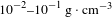 $10^{-2}{-}10^{-1}~\text{g}\cdot \text{cm}^{-3}$
and electron temperatures between 15 and 29 eV, the criterion is fulfilled for temperatures larger than 20 eV and between 10 and 15 eV, for the entire range of mass densities. According to the radiation-hydrodynamics simulations, the peaks in the mass density are located in the rear of the post-shock medium where, according to the simulations for times later than 16 ns, the temperature is approximately 15 eV. Therefore, from the theoretical analysis it is possible that these increases in mass density could be due to thermal instabilities. In addition, the electron temperatures just behind the shock front are higher than 20 eV and, since the criterion is also fulfilled, isobaric thermal instabilities could grow in the shock front, which could be related to the ripples observed in the simulations. However, a clear confirmation would require numerical simulation with radiation turned off, in order to assess whether the instabilities are due to radiative cooling, and also an experimental measure of the length of the initial seeding perturbation, that should be of the order of the sound crossing length for isobaric thermal instabilities.
$10^{-2}{-}10^{-1}~\text{g}\cdot \text{cm}^{-3}$
and electron temperatures between 15 and 29 eV, the criterion is fulfilled for temperatures larger than 20 eV and between 10 and 15 eV, for the entire range of mass densities. According to the radiation-hydrodynamics simulations, the peaks in the mass density are located in the rear of the post-shock medium where, according to the simulations for times later than 16 ns, the temperature is approximately 15 eV. Therefore, from the theoretical analysis it is possible that these increases in mass density could be due to thermal instabilities. In addition, the electron temperatures just behind the shock front are higher than 20 eV and, since the criterion is also fulfilled, isobaric thermal instabilities could grow in the shock front, which could be related to the ripples observed in the simulations. However, a clear confirmation would require numerical simulation with radiation turned off, in order to assess whether the instabilities are due to radiative cooling, and also an experimental measure of the length of the initial seeding perturbation, that should be of the order of the sound crossing length for isobaric thermal instabilities.
5 Conclusions
In this work we have analyzed the radiative and spectroscopic properties of both the radiative precursor and the post-shock medium of radiative shocks driven into xenon by a piston ablated by the Orion high-power laser. The plasma conditions used for the microscopic simulations were extracted from radiation-hydrodynamics simulations. From the analysis of the thermodynamic regime, we have concluded that the xenon plasma, both in the radiative precursor and the post-shock regions, could be assumed to be in LTE. The CSDs were calculated for plasma conditions achieved in the experiments, yielding a maximum average ionization of
 $10$
. This relatively low ionization implies that xenon ions with a large number of bound electrons are present in the plasma which results in complex spectra. The effect of the surrounding plasma on the ion populations was studied, including the CL in the CRSS simulations. The electron densities achieved in the radiative precursor are not too large, but since the electron temperatures are relatively low, plasma effects should still be considered. These effects are more noticeable in the post-shock medium since the mass density is considerably larger than in the radiative precursor whereas the temperatures are similar in the two regions. Furthermore, the CSDs in the post-shock medium are quite similar to those obtained in the radiative precursor, even though the temperatures in the latter can be lower, due to the increased recombination in the post-shock medium. The monochromatic opacities for several characteristic temperatures found in the radiative precursor were analyzed since the outgoing radiation of the plasma can be transported through this region before reaching a detector. This analysis allowed the plasma absorption to be characterized in terms of temperature, which helps to study the plasma spectra.
$10$
. This relatively low ionization implies that xenon ions with a large number of bound electrons are present in the plasma which results in complex spectra. The effect of the surrounding plasma on the ion populations was studied, including the CL in the CRSS simulations. The electron densities achieved in the radiative precursor are not too large, but since the electron temperatures are relatively low, plasma effects should still be considered. These effects are more noticeable in the post-shock medium since the mass density is considerably larger than in the radiative precursor whereas the temperatures are similar in the two regions. Furthermore, the CSDs in the post-shock medium are quite similar to those obtained in the radiative precursor, even though the temperatures in the latter can be lower, due to the increased recombination in the post-shock medium. The monochromatic opacities for several characteristic temperatures found in the radiative precursor were analyzed since the outgoing radiation of the plasma can be transported through this region before reaching a detector. This analysis allowed the plasma absorption to be characterized in terms of temperature, which helps to study the plasma spectra.
The specific intensities of radiation emitted by the radiative precursor and the post-shock medium were also analyzed. For the range of plasma temperatures reached in these experiments, the absorption and emission spectra are in the UV and XUV ranges of photon energies. For the analysis of the intensity, the analysis of the CSDs and the monochromatic opacities and emissivities carried out in this work were very helpful. We have determined that some structures detected in the spectra allow the ranges of plasma temperatures to be predicted, which are associated with ions present in the plasma. However, for the range of electron temperatures 15–20 eV, the CSDs are similar and thus it is difficult to distinguish contributions from different temperatures in that range of temperatures. Therefore, from the spectra we could only conclude that there are regions in the plasma with temperatures in the range 15–20 eV. On the other hand, due to the strong dependence of the first charge states of xenon on temperature, it is easier to distinguish contributions from different temperatures in the range 2–10 eV.
We have also analyzed the intensity of radiation emitted by the post-shock medium. Since the mass density is considerably higher than in the radiative precursor, lines are collisionally broadened, resulting in lines overlapping, and individual lines cannot be identified. This could allow us to estimate the plasma density in the post-shock medium.
Finally, a theoretical analysis of the isobaric thermal instability was made in order to explain the instabilities observed in rad-hydro simulations. Since the criterion of this instability is fulfilled, this could be responsible for the double peaks and ripples observed in the simulations. However, confirmation would require both simulations with radiation turned off and experimental measurements of the length of the seeding perturbations.
Acknowledgements
This work has been supported by the EUROfusion Consortium TASK AGREEMENT WPENR: Enabling Research IFE, Project No. AWP15-ENR-01/CEA-02, by the Project of the Spanish Government with reference FIS2016-81019-P and Labex PLAS@PAR (ANR-11-IDEX-0004-02). The authors would also like to acknowledge the Orion Academic Access programme from which the experimental data was acquired.


 Open access