


Social media summary
Healthy ecosystems are critical for combating climate change.
1. Introduction
The global environment that we experience today is a product of millions of years of co-evolution of climate and the biosphere (Lenton et al., Reference Lenton, Schellnhuber and Szathmáry2004). Concern over human perturbations of the environment (such as water use, the introduction of novel substances into the environment, interference in biogeochemical cycles and land-use change) frequently stems from concern about how these perturbations impact the ability of the climate or the biosphere to support humans. Although interactions between the biosphere and the physical climate system are critical in determining the state of the Earth system, ecosystem-level feedbacks between the biosphere and climate system are not routinely included in projections of or policy for climate change. For example, biodiversity conservation is seen at best as a co-benefit of carbon sequestration measures, not as a strategy that could mitigate further climate change (Díaz et al., Reference Díaz, Wardle, Hector, Naeem, Bunker, Hector, Loreau and Perring2009); projections of greenhouse gas releases from degrading permafrost soils, which comprise a loss of integrity of tundra biomes, are based on simplified approaches (Koven et al., Reference Koven, Schuur, Schädel, Bohn, Burke, Chen and Turetsky2015) and not part of Earth system models (Ciais et al., Reference Ciais, Sabine, Bala, Bopp, Brovkin, Canadell, Thornton, Stocker, Qin, Plattner, Tignor, Allen, Boschung and Midgley2013); and responses of marine ecosystems to acidification and temperature are considered important but rarely included in Earth system models (Ciais et al., Reference Ciais, Sabine, Bala, Bopp, Brovkin, Canadell, Thornton, Stocker, Qin, Plattner, Tignor, Allen, Boschung and Midgley2013).
In the planetary boundary framework (Steffen et al., Reference Steffen, Richardson, Rockström, Cornell, Fetzer, Bennett and Sörlin2015), which delimits the biophysical conditions needed to maintain the Earth system in a ‘safe’ Holocene-like state, the two ‘core’ planetary boundaries of climate change and biosphere integrity represent the geosphere and the biosphere of the Earth system (Steffen et al., Reference Steffen, Richardson, Rockström, Cornell, Fetzer, Bennett and Sörlin2015). We use the terminology of ‘biosphere integrity’, broadly defined as the long-term maintenance of key structures and functions of the biosphere (Steffen et al., Reference Steffen, Richardson, Rockström, Cornell, Fetzer, Bennett and Sörlin2015), as this emphasizes that aspects of the biosphere at multiple scales beyond individual plant physiology, such as ecosystem functioning, are crucial for climate–biosphere interactions. Here, we are specifically interested in ecosystem functions related to climate and the carbon cycle such as the capacity to take up carbon and the capacity to respond to climate change. Biosphere integrity builds on earlier concepts such as biological integrity (Karr, Reference Karr1990), ecological integrity (Mora, Reference Mora2017; Parrish et al., Reference Parrish, Braun and Unnasch2003) and ecosystem integrity (Dorren et al., Reference Dorren, Berger, Imeson, Maier and Rey2004) by viewing this ‘integrity’ at the scale of the Earth system.
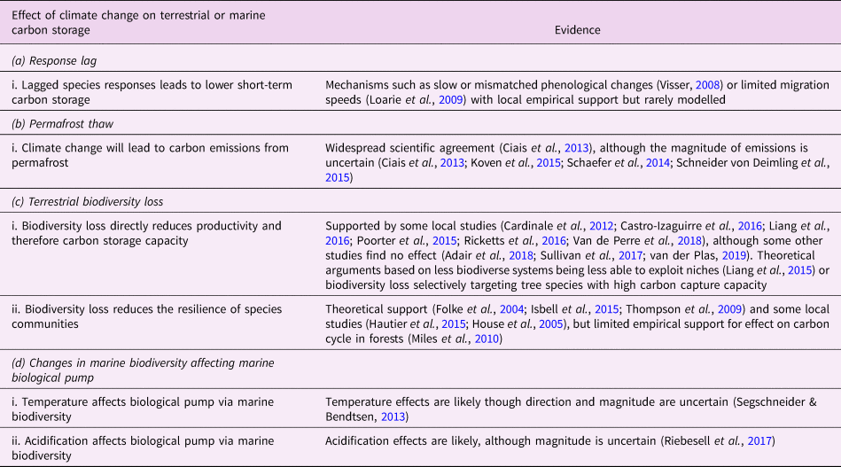
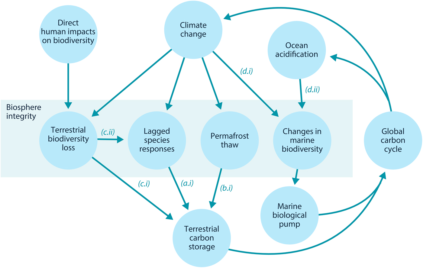
Here, we examine how loss of biosphere integrity could generate significant feedbacks to the climate system on policy-relevant timescales of twenty-first-century climate change. This initial study considers only climate–biosphere interactions involving carbon storage, ignoring other biosphere feedbacks such as albedo changes or changes to the hydrological cycle that could also impact climate (Chapin et al., Reference Chapin, Randerson, McGuire, Foley and Field2008). We focus on the effects of four categories of biosphere integrity loss on carbon storage that are not commonly included in comprehensive global models (Figure 1): (1) Impairment of the capacity of terrestrial ecosystems to store carbon due to lagged responses to climate change. Lagged species responses are known to be an important feature of the terrestrial biosphere's response to climate change (Loarie et al., Reference Loarie, Duffy, Hamilton, Asner, Field and Ackerly2009; Wieczynski et al., Reference Wieczynski, Boyle, Buzzard, Duran, Henderson, Hulshof and Savage2019), although the magnitude of its effect on the carbon cycle is uncertain. (2) Release of carbon from thawing permafrost. The failure of tundra ecosystems to adapt to climate change is expected to release large amounts of carbon (Chadburn et al., Reference Chadburn, Burke, Cox, Friedlingstein, Hugelius and Westermann2017; Ciais et al., Reference Ciais, Sabine, Bala, Bopp, Brovkin, Canadell, Thornton, Stocker, Qin, Plattner, Tignor, Allen, Boschung and Midgley2013; Koven et al., Reference Koven, Schuur, Schädel, Bohn, Burke, Chen and Turetsky2015; MacDougall et al., Reference MacDougall, Zickfeld, Knutti and Matthews2015; Schaefer et al., Reference Schaefer, Lantuit, Romanovsky, Schuur and Witt2014; Schneider von Deimling et al., Reference Schneider von Deimling, Grosse, Strauss, Schirrmeister, Morgenstern, Schaphoff and Boike2015; Schuur et al., Reference Schuur, McGuire, Schädel, Grosse, Harden, Hayes and Vonk2015). Detailed land surface models of permafrost have advanced understanding of potential greenhouse gas releases (Burke et al., Reference Burke, Chadburn and Ekici2017; Ekici et al., Reference Ekici, Beer, Hagemann, Boike, Langer and Hauck2014; Guimberteau et al., Reference Guimberteau, Zhu, Maignan, Huang, Chao, Dantec-Nédélec and Ciais2018; Lawrence et al., Reference Lawrence, Koven, Swenson, Riley and Slater2015; Porada et al., Reference Porada, Ekici and Beer2016), but these models are rarely incorporated into comprehensive global models (Ciais et al., Reference Ciais, Sabine, Bala, Bopp, Brovkin, Canadell, Thornton, Stocker, Qin, Plattner, Tignor, Allen, Boschung and Midgley2013; Hagemann et al., Reference Hagemann, Blome, Ekici and Beer2016). (3) Effects of terrestrial biodiversity loss both directly on productivity and indirectly via reduced resilience. Biodiversity loss is a major global environmental problem (Cardinale et al., Reference Cardinale, Duffy, Gonzalez, Hooper, Perrings, Venail and Naeem2012; House et al., Reference House, Brovkin, Betts, Constanza, Assunçao, Dias, Nishioka, Hassan, Scholes and Ash2005), which could have significant impacts on carbon storage, though the degree to which biodiversity loss will impact the global carbon cycle remains uncertain. Spatially explicit global vegetation models such as LPJmL (Schaphoff et al., Reference Schaphoff, von Bloh, Rammig, Thonicke, Biemans, Forkel and Waha2018) capture major biogeophysical and biogeochemical controls on the dynamic distributions of a few plant functional types, but they include limited aspects of biodiversity (Prentice et al., Reference Prentice, Bondeau, Cramer, Harrison, Hickler, Lucht, Sykes, Canadell, Pataki and Pitelka2007). Local models such as forest succession models (Morin et al., Reference Morin, Fahse, Jactel, Scherer-Lorenzen, García-Valdés and Bugmann2018) can display realistic biodiversity effects but would be difficult to implement at the global scale. New kinds of global ecosystem models, such as the Madingley model (Purves et al., Reference Purves, Scharlemann, Harfoot, Newbold, Tittensor, Hutton and Emmott2013), focus on generic properties of dynamic ecosystems, but these detailed models face computational and parameterization challenges in linking to global biogeophysical and biogeochemical dynamics. (4) Changes in the marine biological pump due to changes in marine biodiversity. The marine biological pump, which transports carbon from the upper ocean to the deep ocean, is an important part of the global carbon cycle. Changes to marine biodiversity caused by climate change may affect the strength of this pump (Beaugrand et al., Reference Beaugrand, Edwards and Legendre2010; Riebesell et al., Reference Riebesell, Bach, Bellerby, Monsalve, Boxhammer, Czerny and Schulz2017; Segschneider & Bendtsen, Reference Segschneider and Bendtsen2013), but the consequences of changes in marine biodiversity are rarely included in comprehensive global models (Ciais et al., Reference Ciais, Sabine, Bala, Bopp, Brovkin, Canadell, Thornton, Stocker, Qin, Plattner, Tignor, Allen, Boschung and Midgley2013).

Fig. 1. Relationships between biosphere integrity mechanisms. The four items within the central box are the four types of biosphere integrity loss considered here. In this model, these biosphere integrity mechanisms participate in a feedback with the global carbon cycle.
Since the biosphere integrity mechanisms listed above are difficult to implement in comprehensive global models, we here take an approach at the opposite extreme of complexity. We extend a globally aggregated climate–carbon cycle model (Lade et al., Reference Lade, Donges, Fetzer, Anderies, Beer, Cornell and Steffen2018) to estimate the potential magnitudes of globally aggregated feedbacks between biosphere integrity and climate change. We assess the strengths of these mechanisms using metrics developed for climate–carbon cycle feedbacks (Friedlingstein et al., Reference Friedlingstein, Bopp, Ciais, Dufresne, Fairhead, LeTreut and Orr2001, Reference Friedlingstein, Cox, Betts, Bopp, Von Bloh, Brovkin and Zeng2006; Gregory et al., Reference Gregory, Jones, Cadule and Friedlingstein2009; Zickfeld et al., Reference Zickfeld, Eby, Matthews, Schmittner and Weaver2011). Our model and its results are not intended to be definitive predictions, but rather to stimulate discussion and research on the role of biosphere integrity in climate change.
2. Methods
To model interactions between biosphere integrity and climate, we modified the climate–carbon cycle model of Lade et al. (Reference Lade, Donges, Fetzer, Anderies, Beer, Cornell and Steffen2018). This model studies the dynamics of globally aggregated carbon stocks (in PgC) on land, c t, in the atmosphere, c a, and in the ocean mixed layer, c m, as well as global mean surface temperature relative to pre-industrial ΔT = T − T 0 (in K). The model represents exchanges of carbon between atmosphere and land via net primary production, respiration and carbon emissions from land-use change, and between atmosphere and the ocean mixed layer via diffusion of carbon dioxide. Global mean surface temperature responds in the model to changing atmospheric carbon stocks with a specified climate sensitivity and with a time lag due to ocean heat capacity. Carbon dioxide is released into the atmosphere by fossil fuel combustion according to the representative concentration pathway (RCP) scenarios and is exported to the deep ocean by the solubility pump. The model includes climate–carbon and concentration–carbon feedbacks (Friedlingstein et al., Reference Friedlingstein, Bopp, Ciais, Dufresne, Fairhead, LeTreut and Orr2001) since the processes that exchange carbon between different pools in the model depend on atmospheric carbon stocks (specifically, net primary productivity and ocean–atmosphere diffusion) and temperature (terrestrial respiration, the solubility pump and the solubility of CO2 in the ocean).
There are many simple models that are used to gain a deeper understanding of climate–carbon cycle feedbacks and that can even emulate the outputs of comprehensive coupled atmosphere–ocean and carbon cycle models (Anderies et al., Reference Anderies, Carpenter, Steffen and Rockström2013; Gasser et al., Reference Gasser, Ciais, Boucher, Quilcaille, Tortora, Bopp and Hauglustaine2017; Gregory et al., Reference Gregory, Jones, Cadule and Friedlingstein2009; Joos et al., Reference Joos, Bruno, Fink, Siegenthaler, Stocker, Le Quere and Sarmiento1996; Meinshausen et al., Reference Meinshausen, Smith, Calvin, Daniel, Kainuma, Lamarque and van Vuuren2011a, Reference Meinshausen, Wigley and Raper2011b; Raupach, Reference Raupach2013; Raupach et al., Reference Raupach, Canadell, Ciais, Friedlingstein, Rayner and Trudinger2011). We specifically used the model of Lade et al. (Reference Lade, Donges, Fetzer, Anderies, Beer, Cornell and Steffen2018) as a starting point because:
• Its global aggregation of carbon stocks is of appropriate complexity for the coarse-grained biosphere integrity mechanisms we seek to include.
• It includes aggregated representations of key carbon cycle processes. For example, Raupach's Simple Carbon–Climate Model (Raupach, Reference Raupach2013; Raupach et al., Reference Raupach, Canadell, Ciais, Friedlingstein, Rayner and Trudinger2011) uses multiple greenhouse gases, but does not include a mechanism-based description of the marine component of the carbon cycle such as the solubility and biological carbon pumps.
• It models processes relevant on our timescale of interest, a policy-relevant timescale to 2100.
• It emulates the results of more complex models to within model spread. Specifically, in Lade et al. (Reference Lade, Donges, Fetzer, Anderies, Beer, Cornell and Steffen2018), the future carbon stocks and temperatures generated by the model were tested against historical changes and the future projections of comprehensive climate–carbon models as reported by the Intergovernmental Panel on Climate Change (IPCC) Fifth Assessment Report (AR5) (Ciais et al., Reference Ciais, Sabine, Bala, Bopp, Brovkin, Canadell, Thornton, Stocker, Qin, Plattner, Tignor, Allen, Boschung and Midgley2013; Collins et al., Reference Collins, Knutti, Arblaster, Dufresne, Fichefet, Friedlingstein, Wehner, Stocker, Qin, Plattner, Tignor, Allen, Boschung and Midgley2013). The results of the model were also tested against the various climate–carbon cycle feedback metrics reported by Arora et al. (Reference Arora, Boer, Friedlingstein, Eby, Jones, Christian and Wu2013), Friedlingstein et al. (Reference Friedlingstein, Cox, Betts, Bopp, Von Bloh, Brovkin and Zeng2006) and Zickfeld et al. (Reference Zickfeld, Eby, Matthews, Schmittner and Weaver2011).
In this section, we review Lade et al.’s model and describe our modifications to account for the biosphere integrity mechanisms in Table 1. These mechanisms in turn result in the new climate–carbon cycle feedbacks shown in Figure 1. Loss of biosphere integrity occurs when these mechanisms are activated: when species responses lag behind climate change, leading to loss of terrestrial carbon (a.i); when carbon is emitted from permafrost (b.i); when loss of biodiversity occurs, leading in turn to loss of capacity to take up carbon (c.i) or capacity to respond to climate change (c.ii); or when temperature changes (d.i) or ocean acidification (d.ii) cause changes in marine biodiversity that weaken the marine biological pump. Undisturbed biosphere integrity therefore corresponds to no lags in species responses, no carbon emitted from permafrost, no loss of biodiversity and no weakening of the biological pump due to changes in marine biodiversity. We reiterate that some of these mechanisms are highly controversial and their quantitative characteristics are highly unconstrained.
Table 1. Relationships between climate change and the biosphere. This is a limited selection of the literature and is not intended to be exhaustive.
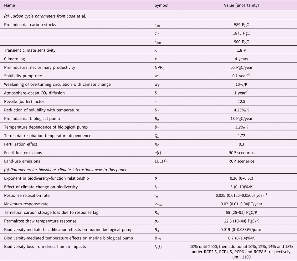
A complete list of parameters is available in Table 2. Two new parameters (K A, Q p) were sufficiently well constrained that we could estimate plausible upper and lower bounds for those parameters. Those uncertainty estimates are described below. For all other new parameters, we estimated their uncertainty using the procedure described in Section 2.5.
Table 2. Model parameters and inputs. All parameters in (a) are from Lade et al. (Reference Lade, Donges, Fetzer, Anderies, Beer, Cornell and Steffen2018); sources for (b) are described in the text. Uncertainties were only estimated for the new parameters for this paper, (b).
2.1. Land
We added to the model of Lade et al. (Reference Lade, Donges, Fetzer, Anderies, Beer, Cornell and Steffen2018) three factors affecting terrestrial carbon storage: response lag, biodiversity loss and permafrost thaw.
2.1.1. Response lag
Changes in plant photosynthesis and plant and soil respiration rates due to climate change are commonly included in comprehensive Earth system models, although large uncertainties remain about their responses to future climates (Ahlström et al., Reference Ahlström, Xia, Arneth, Luo and Smith2015; Arora et al., Reference Arora, Boer, Friedlingstein, Eby, Jones, Christian and Wu2013). Other processes may, however, limit the rate at which species communities can respond in time (such as phenology (Xia et al., Reference Xia, Niu, Ciais, Janssens, Chen, Ammann and Luo2015) and community trait responses (Norberg et al., Reference Norberg, Swaney, Dushoff, Lin, Casagrandi and Levin2001)) and in space (such as range shifts (Davis & Shaw, Reference Davis and Shaw2001)) to climate change (Essl et al., Reference Essl, Dullinger, Rabitsch, Hulme, Pyšek, Wilson and Richardson2015; Svenning & Sandel, Reference Svenning and Sandel2013) (Table 1a.i), particularly to the present very rapid rate of climatic change (Gaffney & Steffen, Reference Gaffney and Steffen2017). Slow or unsynchronized changes in phenology could severely disrupt ecosystem functioning. For example, shifts in insect hatching dates or the timing of vegetation development (Visser, Reference Visser2008) can disrupt interactions such as plant–pollinator relationships (Memmott et al., Reference Memmott, Craze, Waser and Price2007), in turn diminishing the ecosystem's primary productivity (Xia et al., Reference Xia, Niu, Ciais, Janssens, Chen, Ammann and Luo2015). Changes in the spatial distribution of climate patterns will render some species communities unsuited to their current location, which together with limited rates of migration (Settele et al., Reference Settele, Scholes, Betts, Bunn, Leadley, Nepstad, Taboada, Field, Barros, Dokken, March, Mastandrea, Bilir and White2015) may also significantly affect carbon storage (Ahlström et al., Reference Ahlström, Xia, Arneth, Luo and Smith2015).
The species trait modelling of Norberg (Reference Norberg2004) introduces a state variable z that represents the optimal temperature for the growth rate of a species and may lag behind the current temperature T. By analogy, we introduce a state variable z that represents the global mean surface temperature to which global distributions of species are currently best adapted. The magnitude of the difference |Δz − ΔT| is then the response lag. Note that Δz = z – z 0 is different from the Δ defined in Enquist et al. (Reference Enquist, Norberg, Bonser, Violle, Webb, Henderson and Savage2015). We characterize the change in z, Δz, in response to changes in temperature ΔT with two parameters as follows: the response rate r g, where 1/r g gives the response timescale in response to small temperature perturbations. Ecosystems likely also have a maximum rate of response, which we parameterize with v max. We therefore write:
 $$\displaystyle{{d\Delta z} \over {dt}} = v_{{\rm max}}H\lpar {\Delta T,\Delta z} \rpar \tanh \displaystyle{{r_g\lpar {\Delta T-\Delta z} \rpar } \over {v_{{\rm max}}}}.$$
In the absence of any other more plausible functional form, we chose the tanh function to ensure a linear response − r g(ΔT − Δz) for small ΔT − Δz and a constant v max for large ΔT − Δz. The function H represents a biodiversity-dependent further slowing of species responses, to be explained in further detail below. We assume that failure to respond to climatic changes sufficiently quickly – that is, a Δz <ΔT – leads to a temporary loss of aggregated terrestrial carbon carrying capacity given by:
 $$K_A\vert {\Delta T-\Delta z} \vert. $$
This formulation assumes that if ecosystem response Δz can at some point in the future ‘catch up’ to temperature changes ΔT, then carbon storage will return to full capacity.
We calibrated r g = 0.025 yr−1 to match the observation that species migration and community composition responses over the second half of the twentieth century have been approximately half the rate of climate change – that is, Δz/ΔT ≈ 0.5 (Ash et al., Reference Ash, Givnish and Waller2016; Bertrand et al., Reference Bertrand, Lenoir, Piedallu, Riofrío-Dillon, De Ruffray, Vidal and Gégout2011). For v max, we note that the current velocity of climate change (Loarie et al., Reference Loarie, Duffy, Hamilton, Asner, Field and Ackerly2009) already exceeds most historical migration speeds (Davis & Shaw, Reference Davis and Shaw2001). We assume that ecosystems can adapt to at most v max = 0.2°C/decade (Schellnhuber, Reference Schellnhuber2010).
We estimate the parameter K A, the sensitivity of carbon storage to response lag, as follows: two specific parts of the world's forests that are predicted to lose significant amounts of carbon under near-term climate change are the Amazon rainforest and boreal forests. A recent review by Steffen et al. (Reference Steffen, Rockström, Richardson, Lenton, Folke, Liverman and Schellnhuber2018) found a potential loss of carbon due to Amazon and boreal dieback under 2°C warming of 25 PgC (uncertainty range 15–55 PgC) and 30 PgC (uncertainty range 10–40 PgC). These two carbon sources sum to approximately 55 PgC (uncertainty range 25–95 PgC). Our simulations indicate a lag of |Δz − ΔT| ≈ 1°C after 2°C warming; by Eq. (2) we therefore estimate K A ≈ 55 PgC/K (uncertainty range 25–95 PgC/K). This estimate is consistent with the older result of Solomon and Kirilenko (Reference Solomon and Kirilenko1997), who investigated the difference in carbon storage between the extreme scenarios of no forest migration (Δz = 0, in our terminology) and instant biome migration (Δz = ΔT). They found carbon loss (combined soil and vegetation) under the no migration scenario compared to the instant migration scenario of 50 PgC/K (100 PgC under about 2°C temperature rise). A similar study by Van Minnen et al. (Reference Van Minnen, Leemans and Ihle2000) found a response of 190 PgC/K (500 PgC under 2.7°C temperature rise), which we discard as an outlier.
2.1.2. Biodiversity loss
Biodiversity in terrestrial ecosystems is a critical factor for their primary productivity (Morin et al., Reference Morin, Fahse, Jactel, Scherer-Lorenzen, García-Valdés and Bugmann2018; Weisser et al., Reference Weisser, Roscher, Meyer, Ebeling, Luo, Allan and Eisenhauer2017) and their capacity to sink and store carbon (Zhang et al., Reference Zhang, Niinemets, Sheffield and Lichstein2018). Empirical studies of diversity–functionality relationships have mostly used species richness to measure diversity. To parameterize relationships involving biodiversity, we therefore use species richness, although theoretical arguments indicate measures that account for the functional role of species may more accurately predict ecosystem function (Dıaz & Cabido, Reference Dıaz and Cabido2001). Where available, we use the biodiversity intactness index as a measure of biodiversity, since this abundance-weighted measure may approach the functional effect of species loss more closely than species richness (Mace et al., Reference Mace, Reyers, Alkemade, Biggs, Chapin, Cornell and Woodward2014; Scholes & Biggs, Reference Scholes and Biggs2005; Steffen et al., Reference Steffen, Richardson, Rockström, Cornell, Fetzer, Bennett and Sörlin2015).
We modelled two classes of mechanisms that affect biodiversity. First, human activities such as land-use change and landscape homogenization are directly affecting biodiversity (Pereira et al., Reference Pereira, Leadley, Proença, Alkemade, Scharlemann, Fernandez-Manjarrés and Walpole2010; Pimm et al., Reference Pimm, Jenkins, Abell, Brooks, Gittleman, Joppa and Sexton2014). Second, climate-mediated impacts, such as climatic changes leading to species becoming maladapted to their local climate, will also affect biodiversity (Bellard et al., Reference Bellard, Bertelsmeier, Leadley, Thuiller and Courchamp2012). We coarsely represent the direct (e.g., land clearing) and indirect (via climate change) effects on a globally aggregated measure of biodiversity, I:
 $$I\lpar {\Delta T,\Delta z} \rpar = 1-I_{{\rm CC}}\vert {\Delta T-\Delta z} \vert -I_d\lpar t \rpar,$$
where I d(t) specifies direct human impacts on biodiversity and I CC specifies the effect of climate change on biodiversity per ecosystem climate response lag |ΔT − Δz|. Since terrestrial carbon is stored mostly in plants and soils, we envision the biodiversity modelled here as primarily composed of plant biodiversity. A globally aggregated measure may underestimate the effects of local and functional extinctions, which are likely to be more relevant for relationships between biodiversity and ecosystem function (Hooper et al., Reference Hooper, Adair, Cardinale, Byrnes, Hungate, Matulich and O'Connor2012). On the other hand, introduced species could mitigate the impact of global biodiversity loss by locally increasing species diversity (Sax & Gaines, Reference Sax and Gaines2003).
For direct human impacts on biodiversity, I d(t), we assumed a conservative scenario of 10% loss from pre-industrial conditions until 2000, based on the 15% loss of biodiversity intactness index recently estimated by Newbold et al. (Reference Newbold, Hudson, Arnell, Contu, De Palma, Ferrier and Purvis2016) using 2015 data. Projections of future impacts vary widely; for example, extinction rate estimates vary from 60% per century to a hundred-fold smaller (Pereira et al., Reference Pereira, Leadley, Proença, Alkemade, Scharlemann, Fernandez-Manjarrés and Walpole2010; Pimm et al., Reference Pimm, Jenkins, Abell, Brooks, Gittleman, Joppa and Sexton2014). Here, we accommodate the differences in land-use change among the different RCP scenarios. We use predicted gross land-use transitions as a proxy for direct human impacts on biodiversity since net land-use transitions ignore phenomena that will impact biodiversity such as shifting cultivation (Yue et al., Reference Yue, Ciais, Luyssaert, Li, McGrath, Chang and Peng2018). We extend our historical 10% cumulative biodiversity loss scaled by comparing historical cumulative gross land-use transitions (2857 × 106 km2 over 1500–2000; Hurtt et al., Reference Hurtt, Chini, Frolking, Betts, Feddema, Fischer and Wang2011) with predicted twenty-first-century gross land-use change transitions (2926, 3351, 4072 and 5041 × 106 km2 under RCP2.6, RCP4.5, RCP6 and RCP8.5, respectively; Hurtt et al., Reference Hurtt, Chini, Frolking, Betts, Feddema, Fischer and Wang2011). This scaling yields projected biodiversity losses in the twenty-first century (in addition to historical losses) of 10%, 12%, 14% and 18% under RCP2.6, RCP4.5, RCP6 and RCP8.5, respectively.
The impacts of climate change on biodiversity, I CC, are also uncertain (Bellard et al., Reference Bellard, Bertelsmeier, Leadley, Thuiller and Courchamp2012). Under high-emissions scenarios, climate-mediated loss of vascular plant biodiversity may reach  $5\% $ or more by 2100 (van Vuuren et al., Reference van Vuuren, Sala and Pereira2006). Since our model predicts T − z ≈ 1 by 2100, we set I CC = 5%/K, so that losses reach 5% by 2100. Under this parameterization, climate-mediated effects on biodiversity are initially unlikely to exceed direct human impacts, but may be comparable by 2100, matching the predictions of van Vuuren et al. (Reference van Vuuren, Sala and Pereira2006).
We identified two classes of mechanisms for how biodiversity loss may in turn affect carbon storage (Table 1c). First, while the effect is still controversial, decreased biodiversity has been shown to substantially affect the productivity of forest (Liang et al., Reference Liang, Crowther, Picard, Wiser, Zhou, Alberti and Reich2016) and herbaceous (Weisser et al., Reference Weisser, Roscher, Meyer, Ebeling, Luo, Allan and Eisenhauer2017) ecosystems. For example, biodiversity loss can reduce the ability of an ecosystem to efficiently exploit its niches through the complementarity effect (Liang et al., Reference Liang, Zhou, Tobin, McGuire and Reich2015), although the long-term effect remains uncertain (Cardinale et al., Reference Cardinale, Duffy, Gonzalez, Hooper, Perrings, Venail and Naeem2012). Even highly managed monocultures may be less productive than natural ecosystems encompassing many species (Weisser et al., Reference Weisser, Roscher, Meyer, Ebeling, Luo, Allan and Eisenhauer2017). Other results, however, show no or weak relationships between biodiversity and carbon storage (Adair et al., Reference Adair, Hooper, Paquette and Hungate2018; Sullivan et al., Reference Sullivan, Talbot, Lewis, Phillips, Qie, Begne and Zemagho2017). Second, biodiversity loss may reduce the resilience of species communities to climate change, in the sense that a reduced diversity of organisms is available to exploit new climatic conditions in their current location or to migrate to a new location (Miles et al., Reference Miles, Dunning, Doswald and Osti2010).
For the relationship between biodiversity loss and productivity, we use the relationship from Liang et al. (Reference Liang, Crowther, Picard, Wiser, Zhou, Alberti and Reich2016):
 $$\log H\lpar {\Delta T,\Delta z} \rpar = \theta \log I\lpar {\Delta T,\Delta z} \rpar,$$
who found θ = 0.26 (Liang et al., Reference Liang, Crowther, Picard, Wiser, Zhou, Alberti and Reich2016). This relationship is close to the empirical results also found by Hooper et al. (Reference Hooper, Adair, Cardinale, Byrnes, Hungate, Matulich and O'Connor2012) and qualitatively similar to the classic relationship predicted by Naeem (Reference Naeem2002). The initial slope (∂H/∂I = θ = 0.26 at I = 1) is also similar to the linear productivity–functioning fits recently obtained by Morin et al. (Reference Morin, Fahse, Jactel, Scherer-Lorenzen, García-Valdés and Bugmann2018), which are around a third of initial productivity over the full range of biodiversity loss. For the relationship between biodiversity loss and capacity to respond to climate change, we use the same biodiversity–function relationship H(ΔT, Δz) as given by Eq. (4) in the absence of useful empirical relationships. We caution that the biodiversity–function relationship will likely depend on both scale (Thompson et al., Reference Thompson, Isbell, Loreau, O'Connor and Gonzalez2018) and temperature (García et al., Reference García, Bestion, Warfield and Yvon-Durocher2018), factors that we do not include here due to a lack of data.
It remains to incorporate the effects of loss of ecosystem function into the carbon cycle model. In the model of Lade et al. (Reference Lade, Donges, Fetzer, Anderies, Beer, Cornell and Steffen2018), the dynamics of terrestrial carbon is:
 $$\displaystyle{{dc_t} \over {dt}} = \displaystyle{{{\rm NP}{\rm P}_0} \over {c_{t0}}}Q_R^{\Delta T{\rm /}10} \lsqb {K\lpar {c_a,\Delta T,\Delta z} \rpar -c_t} \rsqb -{\rm LUC}\lpar t \rpar, $$
where NPP0 is pre-industrial terrestrial net primary productivity, Q R specifies the temperature dependence of respiration from the terrestrial carbon pool (not including permafrost) and LUC(t) represents carbon emissions due to land-use change. We modify Lade et al.’s expression for terrestrial carbon carrying capacity K to include the effects of response lag and biodiversity loss introduced in Eqs (1–4), giving:
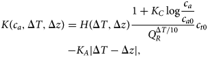 $$\displaylines{K\lpar {c_a,\Delta T,\Delta z} \rpar = H\lpar {\Delta T,\Delta z} \rpar \displaystyle{{1 + K_C\log \displaystyle{{c_a} \over {c_{a0}}}} \over {Q_R^{\Delta T{\rm /}10}}} c_{t0} \cr -K_A\vert {\Delta T-\Delta z} \vert,} $$
From the original model, K C specifies the strength of the response of NPP to CO2, known as the CO2 fertilization effect, and c a0 is the pre-industrial atmospheric carbon stock. The new factor H(ΔT, Δz) of the first term from Eq. (4) models the reduction of carbon storage capacity as a result of biodiversity loss, while the new final term K A|ΔT − Δz| from Eq. (2) models loss of carbon storage due to response lag.
2.1.3. Permafrost thaw
Using the observation that cumulative emissions from permafrost at 2100 under the RCP scenarios (Schneider von Deimling et al., Reference Schneider von Deimling, Grosse, Strauss, Schirrmeister, Morgenstern, Schaphoff and Boike2015) are approximately proportional to increases in global mean surface temperature by 2100 (Collins et al., Reference Collins, Knutti, Arblaster, Dufresne, Fichefet, Friedlingstein, Wehner, Stocker, Qin, Plattner, Tignor, Allen, Boschung and Midgley2013), we model cumulative emission from permafrost with:
 $$c_p = p_T \Delta \lceil T \hskip1pt \rceil. $$
 On the timescales of our model, permafrost thaw is effectively a one-way process: reduction of global mean temperature would not lead to emitted permafrost carbon being reabsorbed. We implement this ‘one-way valve’ through a temperature variable  $\Delta \lceil T \hskip1pt \rceil $ that responds only to temperature increases:
 $$\displaystyle{{ d \lceil T \hskip1pt \rceil } \over {dt}} = \max \left( {\displaystyle{{dT} \over {dt}},0} \right).$$
 The dynamics of temperature T in the model are defined in Section 2.3. We set the initial value of  $ \Delta \lceil T \hskip1pt \rceil $ to 0. We classify permafrost thaw as a loss of biosphere integrity (Table 1b), since permafrost thaw may be considered a failure of tundra ecosystems to maintain their integrity in response to local climate changes (Schmidt et al., Reference Schmidt, Torn, Abiven, Dittmar, Guggenberger, Janssens and Trumbore2011).
We estimated the value of p T as follows: the IPCC AR5 gave an estimate of 50–250 PgC vulnerable to loss as both CO2 and CH4 by 2100 under the high-emissions RCP8.5 scenario (Ciais et al., Reference Ciais, Sabine, Bala, Bopp, Brovkin, Canadell, Thornton, Stocker, Qin, Plattner, Tignor, Allen, Boschung and Midgley2013), equivalent to 14–68 PgC/K. Since the publication of the AR5, there have been several pertinent studies regarding permafrost thawing (Koven et al., Reference Koven, Schuur, Schädel, Bohn, Burke, Chen and Turetsky2015; Schaefer et al., Reference Schaefer, Lantuit, Romanovsky, Schuur and Witt2014; Schneider von Deimling et al., Reference Schneider von Deimling, Grosse, Strauss, Schirrmeister, Morgenstern, Schaphoff and Boike2015). A recent review (Steffen et al., Reference Steffen, Rockström, Richardson, Lenton, Folke, Liverman and Schellnhuber2018) summarized this literature with a figure of 45 PgC (uncertainty range 20–80 PgC) under 2°C warming; that is, a response of p T = 22.5 PgC/K (uncertainty range 10–40 PgC/K).
We caution that this linear approach to emissions from permafrost may be inaccurate for timescales longer than those considered in this study or for scenarios other than the RCP, since in our model emissions from permafrost are not limited by available permafrost carbon stocks. A more accurate and mechanistic treatment would involve explicit modelling of permafrost carbon stocks as well as rates of thawing and emission (Gasser et al., Reference Gasser, Kechiar, Ciais, Burke, Kleinen, Zhu and Obersteiner2018).
2.2. Ocean
The marine biosphere is also closely interlinked with the global carbon cycle. The marine biological pump, alongside the solubility pump, controls the marine carbon cycle. State-of-the-art global models predict that the biological pump may weaken by around 12% by 2100 under an RCP8.5 scenario, due mostly to increased stratification reducing nutrient delivery to the upper ocean and thereby decreasing primary production, although this prediction is uncertain (Bopp et al., Reference Bopp, Resplandy, Orr, Doney, Dunne, Gehlen and Vichi2013). Ocean warming and acidification may additionally shift marine biodiversity towards smaller organisms that are less likely to transport carbon into the deep ocean (Beaugrand et al., Reference Beaugrand, Edwards and Legendre2010; Riebesell et al., Reference Riebesell, Bach, Bellerby, Monsalve, Boxhammer, Czerny and Schulz2017; Segschneider & Bendtsen, Reference Segschneider and Bendtsen2013). Here, we investigated changes to marine biosphere integrity as represented by biodiversity-mediated changes to the biological pump.
For marine carbon, the main change to the model of Lade et al. (Reference Lade, Donges, Fetzer, Anderies, Beer, Cornell and Steffen2018) is to modify the representation of the marine biological pump (which includes the carbonate and soft-tissue pumps). To represent the additional effects of temperature on the biological pump via changes in marine biodiversity, we include an extra temperature-dependent term, B TBΔT. For the effects of acidification, we let B A be the effect of ocean acidification on the strength of the biological pump in units of fractional change relative to pre-industrial conditions per unit change in partial pressure of CO2 in the upper ocean, p(c m, ΔT). We then obtain the final expression for the strength of the biological pump:
 $$B\lpar {\Delta T,p\lpar {c_m,\Delta T} \rpar } \rpar = B_0\lpar {1-B_T\Delta T-B_{TB}\Delta T} \rpar \times \lpar {1-B_A\lsqb {\,p\lpar {c_m,\Delta T} \rpar -c_{a0}} \rsqb } \rpar.$$
We set B A = 0.019%/μatm to match the experimental sedimentation rate results of Riebesell et al. (Reference Riebesell, Bach, Bellerby, Monsalve, Boxhammer, Czerny and Schulz2017). We calibrated B TB = 0.7%/K to match predicted decreased atmosphere to ocean flux of 0.2 PgC/year by 2100 under RCP8.5 (Segschneider & Bendtsen, Reference Segschneider and Bendtsen2013).
The form for B in Eq. (9) can then be used in the existing equation of Lade et al. (Reference Lade, Donges, Fetzer, Anderies, Beer, Cornell and Steffen2018) for the dissolved inorganic carbon content of the ocean mixed layer, c m:
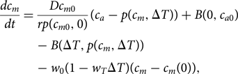 $$\displaystyle{{dc_m} \over {dt}} = \displaystyle{{Dc_{m0}} \over {rp\lpar {c_{m0},0} \rpar }}\lpar {c_a-p\lpar {c_m,\Delta T} \rpar } \rpar + B\lpar {0,c_{a0}} \rpar -B\lpar {\Delta T,p\lpar {c_m,\Delta T} \rpar } \rpar -w_0\lpar {1-w_T\Delta T} \rpar \lpar {c_m-c_m\lpar 0 \rpar } \rpar,$$
in which the partial pressure of CO2 is given by:
 $$p\lpar {c_m,\Delta T} \rpar = c_{a0}\left( {\displaystyle{{c_m} \over {c_{m0}}}} \right)^r\displaystyle{1 \over {1-D_T\Delta T}}.$$
Parameters carried over from Lade et al. (Reference Lade, Donges, Fetzer, Anderies, Beer, Cornell and Steffen2018) are the rate at which the ocean mixed layer is replaced by the solubility pump, w 0; the temperature sensitivity of the solubility pump, w T; the rate of atmosphere–ocean CO2 diffusion, D; the Revelle (buffer) factor for CO2, r; the temperature sensitivity of CO2 solubility, D T; the strength of the pre-industrial biological pump, B 0; the temperature sensitivity of the biological pump, B T; and pre-industrial ocean mixed-layer carbon stock, c m0. The parameter B T represents non-biodiversity-related temperature effects on the biological pump as represented in conventional global models. In Lade et al. (Reference Lade, Donges, Fetzer, Anderies, Beer, Cornell and Steffen2018), B T was estimated from model results in which the biological pump weakens due to a decrease in primary production, in turn due to strengthening thermal stratification of ocean waters (Bopp et al., Reference Bopp, Resplandy, Orr, Doney, Dunne, Gehlen and Vichi2013). Although recent research suggests that depth rather than strength of stratification may be more important for marine productivity (Richardson & Bendtsen, Reference Richardson and Bendtsen2019), we retain the estimate of Lade et al. (Reference Lade, Donges, Fetzer, Anderies, Beer, Cornell and Steffen2018) for consistency.
To calculate the total (surface plus deep) ocean carbon storage, c m, any of several equivalent expressions can be used:
 $$\displaylines{\Delta c_M = \Delta c_m + \int ^tw_0\lpar {1-w_T\Delta T} \rpar \lpar {c_m-c_{m0}} \rpar dt \cr + \int ^t\lpar {B\lpar {\Delta T,p\lpar {c_m,\Delta T} \rpar } \rpar } \rpar -B\lpar {0,c_{a0}} \rpar dt \cr = \int ^tD\lpar {c_{a0}-p\lpar {c_m,\Delta T} \rpar } \rpar dt \cr = \int ^te\lpar t \rpar dt-c_a-c_t + c_{a0} + c_{t0},} $$
where e(t) is the rate of fossil fuel emissions of CO2.
2.3. Atmosphere
We calculate the atmospheric carbon content, c a, by carbon conservation in our ‘system’ composed of carbon stocks in the ocean mixed layer, atmosphere and terrestrial biosphere. Our model has three processes that affect this ‘system carbon’: emissions of fossil carbon into the atmosphere, e(t); export of carbon into the deep ocean by the solubility and biological pumps; and emissions from permafrost carbon. Equation (7) gives cumulative emissions from permafrost, while the other two processes are parameterized in terms of rates. We therefore write:
 $$c_a + c_t + c_m = c_{a0} + c_{t0} + c_{m0} + c_s + c_p,$$
where c s is the change in ‘system carbon’ contributed by fossil fuel emissions and the biological pump. To calculate c s, we solve:
 $$\displaylines{\displaystyle{{dc_s} \over {dt}} = e\lpar t \rpar -w_0\lpar {1-w_T\Delta T} \rpar \lpar {c_m-c_{m0}} \rpar \cr -\,\lpar {B\lpar {\Delta T,p\lpar {c_m,\Delta T} \rpar } \rpar -B\lpar {0,c_{a0}} \rpar } \rpar,} $$
with initial condition c s = 0.
To obtain the dynamics of atmosphere carbon stocks, we therefore solve Eq. (13) and then use the carbon balance equation Eq. (12) to find c a.
The expression for the response of global mean surface temperature T to atmospheric carbon content c a is also unchanged:
 $$\displaystyle{{dT} \over {dt}} = \displaystyle{1 \over \tau} \left( {\displaystyle{\lambda \over {\log 2}}\log \left( {\displaystyle{{c_a} \over {c_{a0}}}} \right)-\Delta T} \right).$$
Parameters carried over from Lade et al. are the climate sensitivity (specifically, transient climate response), λ, and the climate lag, τ.
2.4. Feedback analysis
For many of the biosphere integrity mechanisms introduced above, it is controversial as to whether a mechanism that only has theoretical motivation or only has been observed at small scales actually has a significant impact on the global carbon cycle. Parameterizations of these mechanisms are also often highly unconstrained. We therefore test the potential impacts of each mechanism in turn and one scenario of their potential combined effect where all mechanisms are active.
For each mechanism, we perform one reference simulation with the mechanism ‘switched off’ and then one simulation with the mechanism ‘switched on’. These switches are achieved by changing parameter values to activate and deactivate different mechanisms as listed in Table 3. We include in our analysis the conventional climate–carbon and concentration–carbon feedbacks (Friedlingstein et al., Reference Friedlingstein, Bopp, Ciais, Dufresne, Fairhead, LeTreut and Orr2001, Reference Friedlingstein, Cox, Betts, Bopp, Von Bloh, Brovkin and Zeng2006; Gregory et al., Reference Gregory, Jones, Cadule and Friedlingstein2009; Zickfeld et al., Reference Zickfeld, Eby, Matthews, Schmittner and Weaver2011) analysed by Lade et al. (Reference Lade, Donges, Fetzer, Anderies, Beer, Cornell and Steffen2018), as well as each biosphere integrity mechanism introduced in this paper and one final feedback analysis where all biosphere integrity mechanisms are switched on. To avoid as much as possible the effects of interacting feedbacks, the reference (‘feedback off’) simulations for the biosphere integrity mechanisms have the ocean decoupled when studying land mechanisms and vice versa. We introduce the following definitions for simulation runs that are listed in Table 3:
• Land uncoupled: c t is held constant, which can be achieved by setting K C, LUC(t) = 0 and Q R = 1 in the Lade et al. model and additionally I CC, I d = 0 and Q P = 1 in the full model.
• Ocean CO2 uncoupled: changes in atmospheric carbon concentration do not affect ocean carbon, which can be achieved by replacing c a with c a0 in Eq. (10).
• Ocean uncoupled: c m is held constant, which can be achieved by ‘Ocean CO2 uncoupled’ above together withw T, D T, B T = 0 in the Lade et al. model and additionallyB A, B TB = 0 in the full model.
• Fully uncoupled: both c t and c m are held constant, which can be achieved in the model by using parameters from both ‘Land uncoupled’ and ‘Ocean uncoupled’.
Table 3. Model simulations run for feedback analysis. The feedback ‘off’ model for c.ii is the feedback ‘on’ model for a.i since c.ii modifies the response lag introduced in a.i.

As in Lade et al. (Reference Lade, Donges, Fetzer, Anderies, Beer, Cornell and Steffen2018), changes in Δc a and ΔT are estimated over simulation runs from 1750 to 2100. The model is driven by: historical records and future RCP scenarios (RCP2.6, 4.5, 6 and 8.5) for fossil fuel emissions e(t) and land-use change emissions LUC(t) (Meinshausen et al., Reference Meinshausen, Smith, Calvin, Daniel, Kainuma, Lamarque and van Vuuren2011a) taken from the RCP Database (https://tntcat.iiasa.ac.at/RcpDb); and the scenarios for direct human impacts on biodiversity I d(t) described above and in Table 2. Parameters are as listed in Table 2 except when modified as per individual simulations as listed in Table 3. We note that the model variants studied here are unlikely to match observed historical carbon cycle dynamics as closely as the base model from Lade et al. (Reference Lade, Donges, Fetzer, Anderies, Beer, Cornell and Steffen2018). Recalibrating the model for each run would, however, make assessing the additional warming contributed by each new biosphere integrity mechanism more difficult. We therefore retain Lade et al.’s parameterization throughout.
From the results of these simulations, we estimated three measures for the strength of the mechanisms: (1) the feedback factor (Zickfeld et al., Reference Zickfeld, Eby, Matthews, Schmittner and Weaver2011):
 $$\displaystyle{{\Delta c_a^{{\rm on}}} \over {\Delta c_a^{{\rm off}}}};$$
(2) the additional atmospheric carbon contributed by the mechanism:
 $$\Delta c_a^{{\rm on}} -\Delta c_a^{{\rm off}};$$
and (3) the additional warming contributed by the mechanism:
 $$\Delta T^{{\rm on}}-\Delta T^{{\rm off}},$$
where the superscripts ‘on’ and ‘off’ denote changes with the mechanism active compared to the reference run with the mechanism off. For the feedback factor calculations in Eq. (15), we additionally set biodiversity loss from direct human action I d = 0 and land-use change emissions LUC(t) = 0, since these represent external drivers and not internal climate–carbon feedbacks triggered by fossil fuel emissions.
2.5. Uncertainty analysis
Some parameters (K A, Q p) are sufficiently well constrained that we could estimate plausible upper and lower bounds for those parameters. For other parameters (θ, I CC, B A, B TB), we assigned naïve lower and upper bounds of zero and twice the central parameter estimate, respectively. For multiplicative parameters where a value of zero would have led to model output that did not change over time (r g, v max), we assigned lower and upper bounds of half and twice the central parameter estimate, respectively. These lower and upper bounds are shown in square brackets in Table 2. We did not estimate uncertainty ranges for the parameters inherited from the model of Lade et al. (Reference Lade, Donges, Fetzer, Anderies, Beer, Cornell and Steffen2018) without biosphere integrity mechanisms since (1) uncertainty ranges were not estimated in that study and (2) the purpose of the present study is to estimate the additional feedbacks and warming contributed by biosphere integrity mechanisms, using Lade et al. as a baseline.
We assigned uniform probability distributions to these parameters with the central ‘best estimate’ as the median; that is:
 $$P\lpar x \rpar = \left\{ {\matrix{ {\displaystyle{{0.5} \over {c-l}},} \hfill & {l \lt x \lt c} \hfill \cr {\displaystyle{{0.5} \over {u-c}},} \hfill & {c \lt x \lt u} \hfill \cr {0,} \hfill & {{\rm otherwise}} \hfill \cr}} \right.$$
where l, c and u are the lower bound, central ‘best estimate’ and upper bound of the parameter, respectively. For model runs studying individual biosphere integrity mechanisms, this leads to approximately uniform distributions of the output variable. We therefore plot these results using a bar to indicate the uncertainty range and a marker to indicate the output using the central ‘best estimate’ parameter values. Model runs studying possible total biosphere integrity effects produce a less trivial distribution of the output variable, since this model convolves the uniform distributions of multiple parameters. We present the distributions of the output variables for these models using box-and-whisker plots.
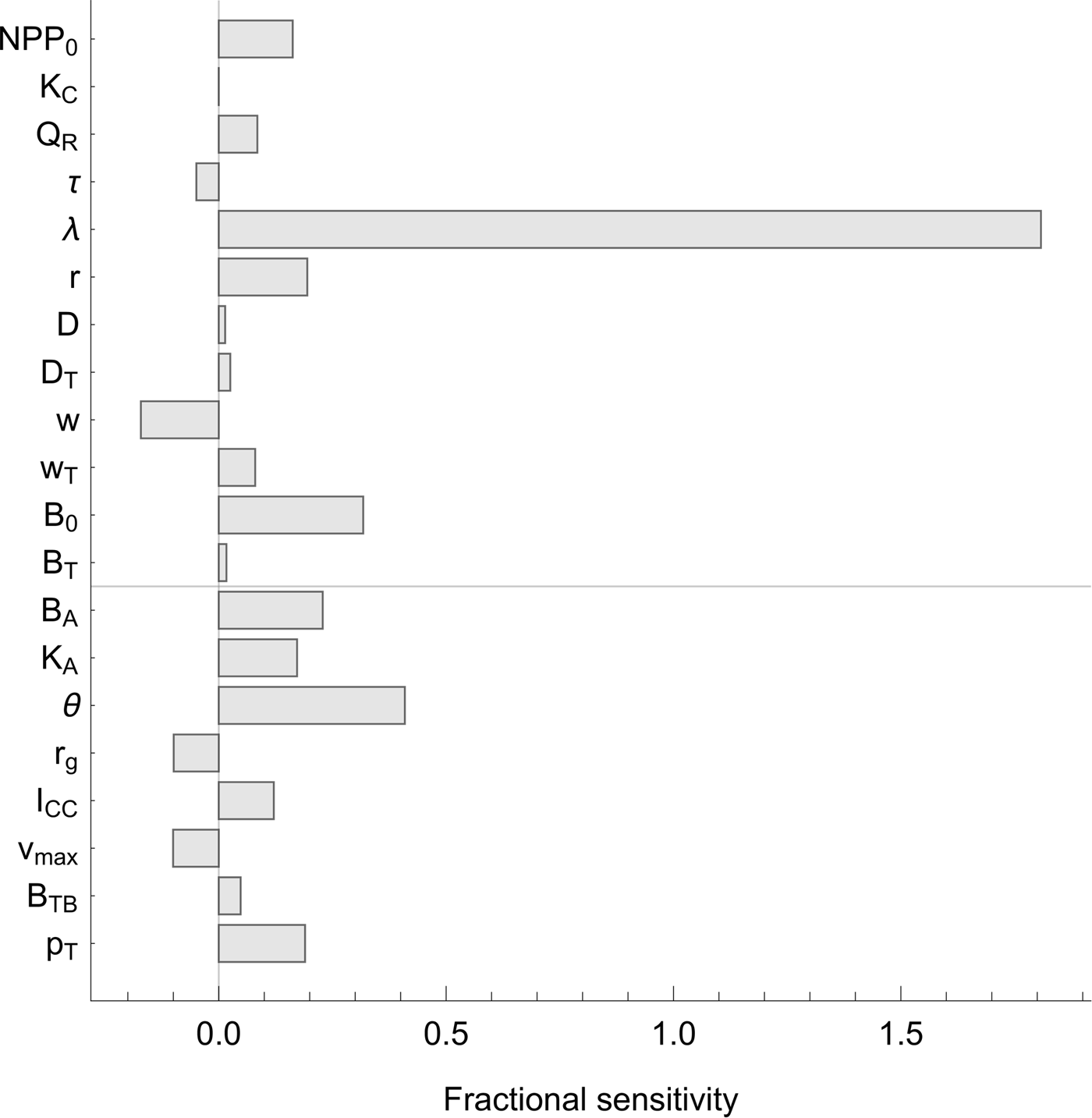
We also performed a sensitivity analysis to test the dependence of the model's results on the parameters of the model. We chose the total additional warming contributed by all biosphere integrity mechanisms under RCP8.5 as a representative result on which to test sensitivity.
3. Results
Using each of the three feedback metrics listed in Eqs (15), (16) and (17), Figure 2 measures: the generic climate–carbon cycle feedbacks analysed by Lade et al. (Reference Lade, Donges, Fetzer, Anderies, Beer, Cornell and Steffen2018) in their baseline model; each new biosphere integrity mechanism introduced in this article; and the total effect of the new biosphere integrity mechanisms. (We did not, however, measure the extra warming contributed by the baseline climate–carbon feedbacks since measuring some of these feedbacks involves disconnecting the climate part of the model.)
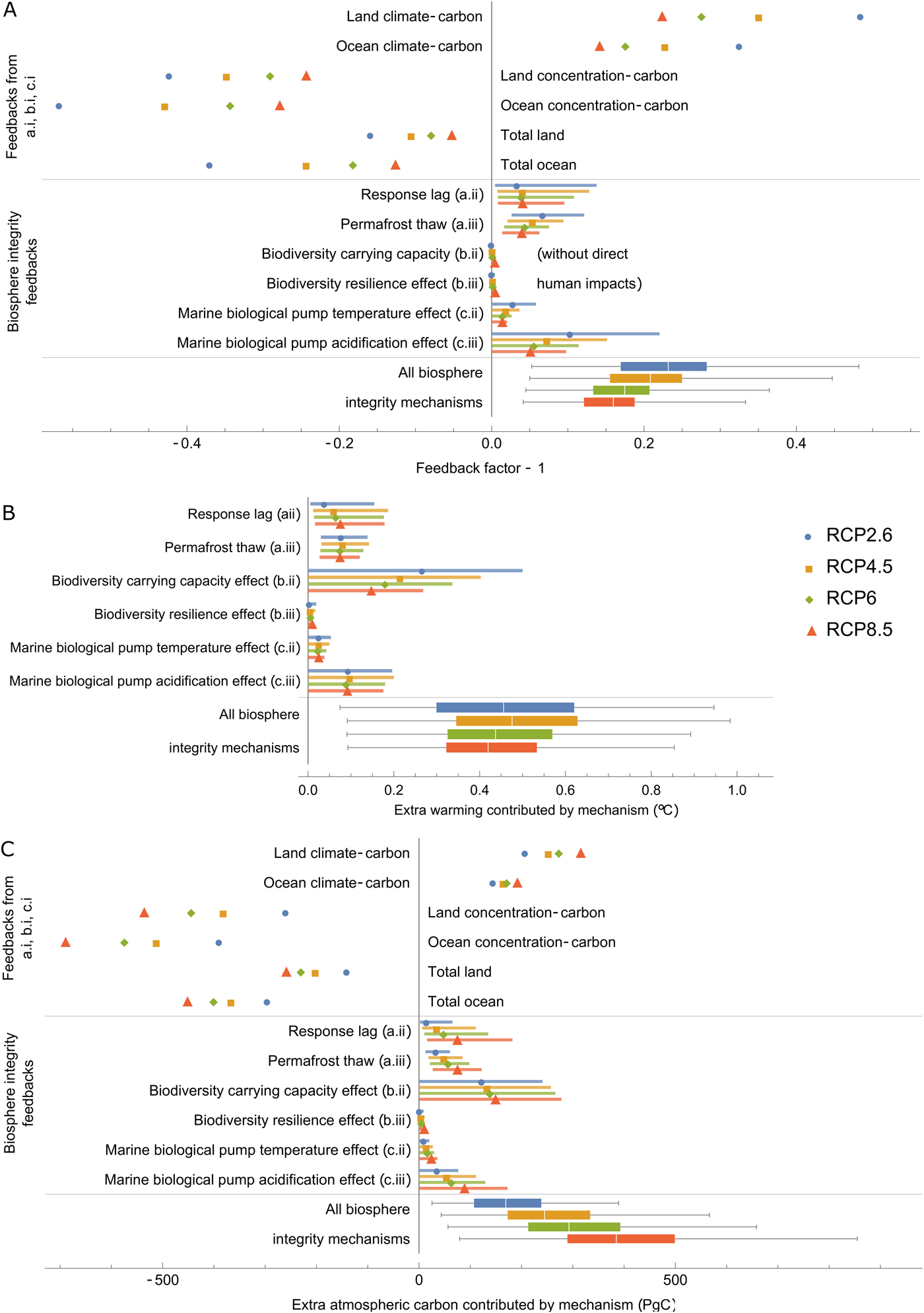
Fig. 2. Results of the climate–carbon cycle–biosphere integrity model. (A) Feedbacks reported by Lade et al. (Reference Lade, Donges, Fetzer, Anderies, Beer, Cornell and Steffen2018) without biosphere integrity feedbacks (top); biosphere integrity feedbacks new to this paper (middle); and total biosphere integrity feedbacks assuming all biosphere integrity mechanisms are active. We plot the feedback factor minus one so that positive numbers correspond to positive (reinforcing) feedbacks and negative numbers correspond to negative (balancing) feedbacks. In this plot, we also set direct biodiversity losses and land-use change emissions to zero (I d(t) = 0 and LUC(t) = 0) so that only endogenous carbon cycle feedbacks to atmospheric carbon changes triggered by fossil fuel emissions are included. (B) Additional warming and (C) additional atmospheric carbon dioxide contributed by losses of biosphere integrity. Labels for different biosphere integrity mechanisms (a.i, b.i, etc.) refer to the list in Table 1.
We caution that the uncertainty ranges associated with the biosphere integrity mechanisms, however, are very large. Permafrost thaw was the only mechanism for which there was empirical support for a non-zero effect. All other mechanisms could have anywhere between zero effect to feedbacks that contributed warming up to several tenths of a degree (Figure 2B). The following results should therefore be treated as well-informed speculation. Quantitative results listed in the text refer to the central ‘best estimates’ produced by our model (see Section 2.5), but for many mechanisms there is substantial uncertainty over whether the mechanism operates at all, let alone its magnitude.
The feedbacks measured in the baseline model (top part of Figure 2A) reproduce the results found in Lade et al. (Reference Lade, Donges, Fetzer, Anderies, Beer, Cornell and Steffen2018). Land and ocean climate–carbon feedbacks (where a change in climate causes a change in land or ocean carbon stocks, respectively, which causes a change in atmospheric carbon and thereby climate) were both positive. In the model, these positive feedbacks occur due to the dependence of terrestrial respiration rates, the marine solubility pump, marine biological pump and ocean CO2 solubility on temperature (Lade et al., Reference Lade, Donges, Fetzer, Anderies, Beer, Cornell and Steffen2018). Land and ocean concentration–carbon feedbacks (where a change in atmospheric carbon causes a change in land or ocean carbon stocks, respectively, which causes a change in atmospheric carbon) were both negative (Figure 2A). In the model, these negative feedbacks occur due to the dependence of terrestrial productivity on CO2 concentration and the diffusion of atmospheric CO2 into the ocean (Lade et al., Reference Lade, Donges, Fetzer, Anderies, Beer, Cornell and Steffen2018). Both land and ocean climate–carbon cycle feedbacks (combing both climate–carbon and concentration–carbon feedbacks) were negative overall, although they were weakest for the extreme RCP8.5 scenario.
All feedback metrics are positive for the new biosphere integrity mechanisms, as expected; that is, they all could contribute additional climate–carbon cycle feedbacks that lead to additional atmospheric carbon stocks and additional climate warming (Figure 2). The biodiversity–productivity effect (c.i) – that is, biodiversity loss leading to reduced productivity and thereby reduced carbon storage – was the strongest mechanism in the warming (Figure 2B) and atmospheric carbon (Figure 2C) metrics according to their central ‘best estimates’. When calculating the feedback factor metric (Figure 2A), we switched off the direct human impacts on biodiversity (I d(t)) since this impact constitutes a driver and not a feedback within the model. This significantly reduced the strength of the biodiversity–productivity effect, indicating that direct human impacts dominate over climate-mediated impacts in the model. The next three largest mechanisms, according to their central estimates, were response lag (a.i), permafrost thaw (b.i) and the marine biological pump acidification effect (d.ii).
The biodiversity–resilience effect (c.ii) was the weakest of the biosphere integrity mechanisms considered here. We speculate that the biodiversity–resilience effect is small because it is a ‘second-order mechanism’, in that it requires both a substantial lag between climate and ecosystem response (ΔT − Δz) and a sufficient biodiversity-mediated increase in response lag (H(ΔT, Δz)) to have developed (see Eq. 1). While a longer simulation may allow these factors to develop, preliminary results indicate that the effect remains small compared to other mechanisms, even on longer timescales. We note, however, that our assumptions for biodiversity loss are also relatively conservative, excluding any explicit biodiversity tipping points or similar mechanisms.
Of the four categories of biosphere integrity mechanisms, the marine effects (d.i and d.ii) were smallest. Their combined effects, which reached central estimates of approximately 0.1°C under all scenarios (Figure 2B), are significant compared to a 1.5°C global goal, but less than from the biosphere integrity mechanisms in the terrestrial biosphere. The 100-year timescale considered here, however, is relatively short for ocean dynamics. On long timescales, the marine biosphere may be the critical factor constraining atmospheric carbon dioxide levels (Sigman & Boyle, Reference Sigman and Boyle2000).
Mirroring the baseline model results, the feedback factors for the biosphere integrity mechanisms were generally the same or slightly smaller for the more extreme RCP scenarios. The extra atmospheric carbon contributed by each mechanism was, however, generally larger for the more extreme RCP scenarios. Feedback factors are the ratio between changes in atmospheric carbon with the mechanism active and inactive. That the extra atmospheric carbon contributed increased with the RCP scenario indicates, therefore, that the reduction in amplification associated with a reduced feedback factor did not outweigh the increase in atmospheric carbon content associated with the greater fossil fuel emissions of the more extreme RCP scenarios. Remarkably, the maximum additional warming (Figure 2B) is roughly the same across the four RCP emissions scenarios. Feedbacks in high-emissions scenarios release more carbon into the atmosphere than in low-emissions scenarios (Figure 2C), but this is balanced by the lower marginal sensitivity of temperature to atmospheric carbon at high atmospheric carbon levels (Myhre et al., Reference Myhre, Highwood, Shine and Stordal1998). That temperature is less sensitive to atmospheric carbon under large carbon emissions, however, does not make mitigating climate change easier; in fact, at high atmospheric carbon levels, greater reductions of carbon emissions will be required to mitigate the same magnitude of warming.
None of the individual biosphere integrity mechanisms are likely to outweigh existing climate–carbon cycle feedbacks and turn the land or ocean into net carbon sources. However, lags in ecosystem response and permafrost thaw could together halve the total land carbon feedback, according to their central estimates (Figure 2A). The combined effects of these feedbacks could generate a positive carbon-cycle feedback, leading to up to an additional 0.1°C or more of warming (Figure 2B), according to their central estimates under all RCP scenarios. About half of this additional warming was due to carbon releases from warming and thawing permafrost soils and half was due to range shifts. The direct impact of biodiversity loss on terrestrial primary production (Table 1c.i) could contribute a warming exceeding 0.2°C (Figure 2B), according to its central estimate under all RCP scenarios, and also contribute an additional positive feedback that, if all terrestrial biosphere integrity mechanisms considered here are active, could exceed the baseline terrestrial carbon sink under all emissions scenarios (compare ‘Total land’ above the line with all terrestrial biodiversity integrity mechanisms in Figure 2C).
The net additional warming of all biosphere integrity mechanisms considered here could exceed 0.4°C (Figure 2B, bottom line), according to their central estimates under all RCP scenarios. This may seem to be a relatively small amount, but it is substantial compared to a 1.5 or 2.0°C target. For example, given a median transient climate response to cumulative emissions of 1.29°C per 1000 GtC (Millar et al., Reference Millar, Fuglestvedt, Friedlingstein, Rogelj, Grubb, Matthews and Allen2017), 0.4°C corresponds to a substantial reduction in allowable cumulative emissions of around 310 GtC independently of the temperature target itself.
The sensitivity analysis (Figure 3) shows that the total additional warming is most sensitive to λ, which is not surprising, as λ controls the sensitivity of temperature change to atmospheric carbon dioxide levels. Of the other parameters, none stands out as exceptionally significant. Of the parameters related to the biosphere integrity mechanisms, total additional warming is most sensitive to θ, which controls the shape of the biodiversity–function relationship.

Fig. 3. Sensitivity analysis. Sensitivity of the central estimate of the total additional warming contributed by all biosphere integrity mechanisms under RCP8.5 (Figure 2B, bottom line) to all model parameters. Sensitivity was computed by increasing and decreasing each parameter in turn by 10% above and below its nominal value. Fractional sensitivity is reported; that is, a value of x indicates that a change in the parameter of  $y\% $ will cause a change in the total warming by $xy\% $ (in the local linear approximation). Parameters above the line indicate those inherited from the baseline model of Lade et al. (Reference Lade, Donges, Fetzer, Anderies, Beer, Cornell and Steffen2018); parameters below the line indicate new parameters.
4. Discussion
We used a stylized global carbon cycle model to study four classes of interactions between biosphere integrity and climate: response lags, permafrost thaw, terrestrial biodiversity loss and changes in marine biodiversity that affect the marine biological pump (Table 1). We found that response lags, permafrost thaw and terrestrial vegetation biodiversity loss could significantly undermine mitigation efforts to reduce fossil fuels emissions. If all of these mechanisms are active, they could lead to land becoming a net carbon source by 2100, according to their central estimates. Marine biosphere integrity mechanisms were the weakest of the four classes of interactions considered here, although this result may be due to the short timescales considered here, as the marine biosphere may be the critical factor constraining atmospheric carbon dioxide levels in the long term (Sigman & Boyle, Reference Sigman and Boyle2000). Many of the biosphere integrity mechanisms studied here are, however, highly unconstrained, and the results should be treated as highly speculative.
Our work points to several arenas of research and policy that could support better understanding and policy-making regarding the interplay between biosphere integrity and climate change. In global modelling, our results suggest that a deeper integration of sophisticated models of the biosphere, incorporating biodiversity, permafrost dynamics and complex ecosystem structure, may be essential for meaningful future assessments of anthropogenic climate change. Such next-generation global biosphere models are becoming available (Purves et al., Reference Purves, Scharlemann, Harfoot, Newbold, Tittensor, Hutton and Emmott2013), but they are not yet coupled to other relevant parts of the Earth system. Our work highlights the need for further research on biodiversity and ecosystem functioning, including how the interplay between range shift speeds, local trait diversity and ecosystem functioning (Isbell et al., Reference Isbell, Gonzalez, Loreau, Cowles, Diaz, Hector and Larigauderie2017; Pecl et al., Reference Pecl, Araújo, Bell, Blanchard, Bonebrake, Chen and Williams2017; Wieczynski et al., Reference Wieczynski, Boyle, Buzzard, Duran, Henderson, Hulshof and Savage2019) can lead to an integrated understanding of biosphere response capacity in relation to climate change (Enquist et al., Reference Enquist, Norberg, Bonser, Violle, Webb, Henderson and Savage2015). In the ocean, while it is traditionally assumed that heavily ballasted phytoplankton are responsible for the majority of carbon transfer via the biological pump, future climate-mediated changes to marine biota may lead to other organisms dominating carbon transfer (Segschneider & Bendtsen, Reference Segschneider and Bendtsen2013).
The interactions and feedbacks between biosphere integrity and climate imply that current global governance of biodiversity and climate change also needs to interact in new ways. The world's societies have acknowledged the importance of the climate and biosphere individually through the United Nations Framework Convention on Climate Change and the Convention of Biological Diversity. To inform these policy processes, scientific advisory bodies have been established: the IPCC and the Intergovernmental Platform on Biodiversity and Ecosystem Services (IPBES). The IPCC's projections of impacts of human activities on climate are based on coupled ocean–atmosphere models of carbon and energy flows that take limited account of the role of biological diversity. IPBES, on the other hand, is currently focused on species, their distributions and their direct benefits to societies; attention to ecosystem functioning and Earth system dynamics is less prominent. The divergent policy priorities of IPCC and IPBES and the use of such disparate currencies as CO2-equivalents and species in their respective science communities and modelling tools preclude the serious exploration of the potential interactions of climate change with the biologically controlled stocks and flows in the global carbon cycle. We call for the work of bodies such as the IPCC and IPBES to be better integrated.
Here, we have undertaken one of the first studies of planetary boundary interactions. The planetary boundary framework has been popular in some sectors of government and business, but the boundaries are conventionally presented as not interacting. We extended a previous stylized carbon cycle model to study the potential feedbacks between the climate change and biosphere integrity planetary boundaries. In addition to climate change causing loss of biosphere integrity, we analysed several mechanisms by which loss of biosphere integrity could accelerate climate change and lead to a significant feedback between climate change and loss of biosphere integrity. Analysing and synthesizing interactions between the planetary boundaries may assist policy-makers in recognizing the importance of interactions between climate change, biosphere integrity and other environmental policy challenges.
Acknowledgements
None.
Author contributions
SJL, JN, JMA, SEC, JFD, IF, KR, JR and WS designed the research. SJL, JN, TG, CB and WS constructed the model. SJL analysed the model. All authors wrote the paper.
Financial support
The research leading to these results has received funding from the Stordalen Foundation via the Planetary Boundary Research Network (PB.net), the Earth League's EarthDoc programme, the Leibniz Association (project DOMINOES), European Research Council Synergy project Imbalance-P (grant ERC-2013-SyG-610028), European Research Council Advanced Investigator project ERA (grant ERC-2016-ADG-743080), Deutsche Forschungsgemeinschaft (DFG BE 6485/1-1), Project Grant 2014-589 from the Swedish Research Council Formas and a core grant to the Stockholm Resilience Centre by Mistra.
Conflicts of interest
None.
Ethical standards
This research and article complies with Global Sustainability’s publishing ethics guidelines.


 Open access