


1. Introduction
All microevolutionary processes produce changes in allele frequencies. Such processes could therefore be detected by analysing the temporal variation in allele frequencies. If this variation is too high to be caused by sampling error and genetic drift alone, it can be inferred that other evolutionary forces are responsible. The tests that are most commonly used to compare samples taken over time are the homogeneity χ2, t, or G tests; analysis of molecular variance (AMOVA); and population divergence statistics (e.g. F ST) (examples in Jorde & Ryman, Reference Jorde and Ryman1995; Viard et al., Reference Viard, Justy and Jarne1997; Laikre et al., Reference Laikre, Jorde and Ryman1998; White et al., Reference White, Kennedy and Kennedy1998; Rank & Dahlhoff, Reference Rank and Dahlhoff2002; Nayar et al., Reference Nayar, Knight and Munstermann2003; Säisä et al., Reference Säisä, Koljonen and Tähtinen2003; Williams et al., Reference Williams, Blejwas, Johnston and Jaeger2003; Han & Caprio, Reference Han and Caprio2004a, Reference Han and Capriob; Kollars et al., Reference Kollars, Beck, Mech, Kennedy and Kennedy2004; Le Clerc et al., Reference Le Clerc, Bazante, Baril, Guiard and Zhang2005). These tests are not completely adequate, because their null hypothesis fails to account for genetic drift (Gibson et al., Reference Gibson, Lewis, Adena and Wilson1979; Waples, Reference Waples1989a), and this may lead to an overestimation of the significance values.
Some tests that have been developed for this purpose so far have had a limited impact, most likely because the majority were developed for specific purposes (examples in Fisher & Ford, Reference Lewontin and Krakauer1947; Lewontin & Krakauer, Reference Lewontin and Krakauer1973; Schaffer et al., Reference Schaffer, Yardley and Anderson1977; Gibson et al., Reference Gibson, Lewis, Adena and Wilson1979; Wilson, Reference Wilson1980; Watterson, Reference Watterson1982; Mueller et al., Reference Mueller, Wilcox, Ehrlich, Heckel and Murphy1985). More recently, Goldringer & Bataillon (Reference Goldringer and Bataillon2004) proposed that using a simulated distribution of Fc,l (the standardized variance in allele frequencies between generations) can be useful for testing temporal changes in allele frequencies. More recently, Bollback et al. (Reference Bollback, York and Nielsen2008) developed a method for estimating Ne and s (selection coefficient) using transition probabilities whose numerical solution could be used for testing temporal changes, too. In addition, Beaumont (Reference Beaumont2003) compared several methods attaining Markov chain Monte Carlo (MCMC) algorithms and importance sampling (IS) for estimating population growth or decline, which also could be used for testing temporal changes in allele frequencies. However, those proposals did not provide the common researcher with a practical way to implement them.
A test for general usage whose implementation was practical was developed by Waples (Reference Waples1989a), and used χ2 adjusted to take into account the genetic drift. Nevertheless, this test may overestimate the probability values with a large number of samples and small population sizes (Waples, Reference Waples1989b). Moreover, implementation of the test is complicated when there are many alleles and samples (Goldringer & Bataillon, Reference Goldringer and Bataillon2004).
In addition, the most frequently used method to model a sample taken from a population is by binomial (replacement) sampling, but the samples should be considered strictly hypergeometric (non-replacement) (Pollak, Reference Pollak1983; Waples, Reference Waples1989b) because, in reality, the sampling rarely implies the return and randomization of an organism to the population before the next organism is taken. Waples’ test overcame that problem by considering the samples as drawn from the previous generation gene pool from which they represent binomial samples (Waples, Reference Waples1989a, Reference Waplesb).
Here, I present a general-use statistical test that is based on computer simulations under a Bayesian background, incorporating binomial sampling for change of generation and hypergeometric sampling for getting effective population and samples, and a user-friendly computer programme that performs the proposed analysis and the Waples test for a number of different scenarios (e.g. multiallelic systems, several samples, N and Ne variables).
2. Materials and methods
(i) The algorithm
Consider a locus with k alleles in a panmictic population with discrete generations of size N and effective population size N e (number of reproductive organisms). Let P 0, …, Pt be the vectors of allele frequencies in the whole population at generations 0, 1, …, t, respectively, and P e0, …, P et the frequency vectors of the effective population of 0, 1, …, t generations. Let X and Y be the frequency vectors in the samples taken at generations 0 and t, with sampling sizes S 0 and St.

where j indicates the generation and the second subindex denotes the allele.
Following Nei & Tajima's (Reference Nei and Tajima1981) and Pollak's (Reference Pollak1983) models, the simplest algorithm compared two samples taken from two consecutive generations as follows (see Fig. 1): after the initial parameters (N, N e, S 0, St) were set, the frequencies in the samples (X and Y) and in the effective population (P e0) were generated with hypergeometric multivariate random vectors, while the next generation frequencies (P 1) were obtained from multinomial deviates. After the process was repeated many times, the frequency of the occasions when the distance between the simulated allele frequencies was larger than the observed one ![]() was taken as the P-value of the test.
was taken as the P-value of the test.
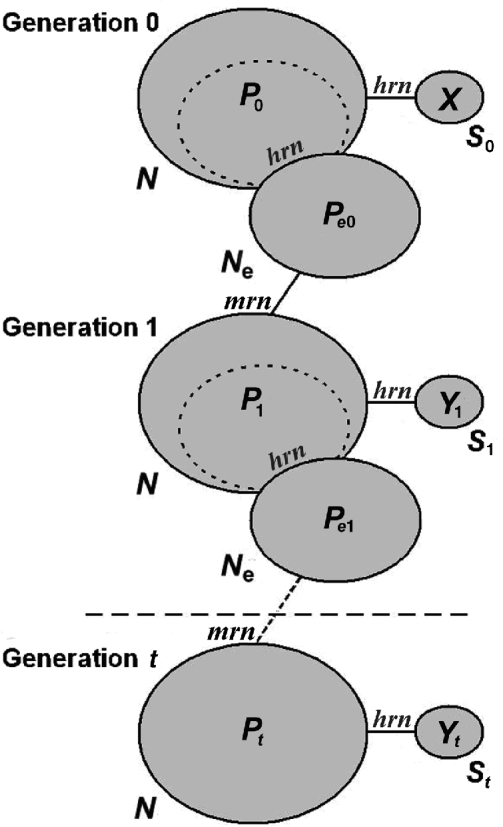
Fig. 1. Model followed by the simulations. Each ellipse represents a population. The size of the population is indicated by the term outside the ellipse, and the allele frequency of one allele at a particular locus is represented by the term inside. The subindex indicates the generation number. The effective population is a splinter group of the total population, as are the samples (they represent non-replacement samples). The total population is obtained by random mating of a very large number of gametes, and therefore, the total population can be modelled as sampling with replacement from the previous effective population. The algorithm substitutes these sampling processes by generating random numbers, whether hypergeometric (hrn) or multinomial (mrn). When the samples are separated by t generations, the intermediate non-sampled generations can be simulated only by a binomial deviate (see text).
The distance between m samples, X, Y 1, Y 2, …, Ym −1 (all taken at different times), had the form ![]() , where Y 0=X. Notice that there is no exponent for the difference since it would make small differences even lower, distorting the magnitude of the differences.
, where Y 0=X. Notice that there is no exponent for the difference since it would make small differences even lower, distorting the magnitude of the differences.
Samples separated by t generations required an additional hypergeometric deviate (for effective population) and a multinomial deviate (for total population) for each additional generation. Alternatively, as other authors have argued, intermediate non-sampled generations could be generated only by multinomial deviates, because an effective population can be considered a multinomial draw from the previous generation (Waples, Reference Waples1989a).
The described procedure dealt with uncertainty about N and N e, and the allele frequencies at generation zero (P 0).
Estimation of N and N e based on the temporally spaced samples would be redundant and clearly incorrect. Instead, two approaches can be performed, and both are suggested here: assaying of several reasonable combinations of N and N e values by using the available knowledge about the population and employing an estimation of N e with a method other than the temporal one, for instance, the Waples & Do (Reference Waples and Do2008) and Hill (Reference Hill1981) linkage disequilibrium methods or Pudovkin et al.'s (Reference Pudovkin, Zaykin and Hedgecock1996) heterozygote excess method, the last two implemented in Ovenden et al.'s (Reference Ovenden, Peel, Street, Courtney and Hoyle2007) Software NeEstimator.
Uncertainty about P 0 required some mathematical treatment (see above).
(ii) Bayesian analysis
For representation simplicity, let us consider only the case of two temporally spaced samples X and Y. A Bayesian approach could use the predictive distribution of the allele frequencies in the samples, ![]() and
and ![]() , conditional to the observed frequencies:
, conditional to the observed frequencies:
Over such distribution, the rejection region would be established as the one with a volume of α, where the distances between ![]() and
and ![]() ,
, ![]() are as high as possible. A better approach could be performed by calculating the P-value by estimating the volume under the curve drawn by eqn (1), where
are as high as possible. A better approach could be performed by calculating the P-value by estimating the volume under the curve drawn by eqn (1), where ![]() is true. Such volume could be obtained only by integrating eqn (1), whose form should be written in terms of the unknown hyperparameter P 0:
is true. Such volume could be obtained only by integrating eqn (1), whose form should be written in terms of the unknown hyperparameter P 0:
Obtaining an analytic closed form for eqn (2) would be quite a problem, since it would require extensive and even intractable integration; however, this problem could be overcome by simulating random deviates from it. Each simulation could be done in two sequential stages: (i) simulating P 0 deviates from f(P 0|X obs, Y obs); and (ii) simulating ![]() and
and ![]() from f(
from f(![]() ,
,![]() |P 0) for every P 0 vector obtained in the first stage, in order to finally calculate
|P 0) for every P 0 vector obtained in the first stage, in order to finally calculate ![]() . This algorithm would actually generate vectors
. This algorithm would actually generate vectors ![]() and
and ![]() from the desired distribution (eqn 2). The algorithm described in section (i) (also modelled in Fig. 1) indeed is valid for the second stage (ii), but the first one (i) has some potential difficulties, as the simulation from the inverse of a hypergeometric multivariate density. Two approaches were used for dealing with the simulation of P 0 from f(P 0|X obs, Y obs): an empirical Bayes (EB) and a fully Bayesian with f(P 0|X obs, Y obs) approached by a more friendly distribution.
from the desired distribution (eqn 2). The algorithm described in section (i) (also modelled in Fig. 1) indeed is valid for the second stage (ii), but the first one (i) has some potential difficulties, as the simulation from the inverse of a hypergeometric multivariate density. Two approaches were used for dealing with the simulation of P 0 from f(P 0|X obs, Y obs): an empirical Bayes (EB) and a fully Bayesian with f(P 0|X obs, Y obs) approached by a more friendly distribution.
EB approaches use the observed data to estimate some intermediate parameter (in this case, P 0) and then proceed as though it was a known quantity (Carlin & Louis, Reference Carlin and Louis2009). Thus, instead of using eqn (2), simulations of ![]() and
and ![]() were drawn from
were drawn from
where ![]() 0 is a moments’ estimator of P 0 done by the method described by Waples (Reference Waples1989a) . In summary, the EB algorithm consists of the following:
0 is a moments’ estimator of P 0 done by the method described by Waples (Reference Waples1989a) . In summary, the EB algorithm consists of the following:
• Calculate
 .
.• Estimate P 0 by using the data from all the samples according to Waples (Reference Waples1989a) .
• Simulate a large number of values of
and from eqn (3) by using the algorithm described in section (i) with the estimation of P 0 as the initial frequencies (the ones of the population at generation zero). For each simulation, calculate and record the number of times when is true;• Finally, the P-value of the test corresponds to the quotient between the number recorded in the simulations and the overall number of simulations generated.
EB procedures could give reliable estimates since the posterior still used the samples’ information but at much lower computational cost (Casella, Reference Casella1985).
The fully Bayesian approach still used simulations from a distribution (eqn 2), but replaces the first stage of the simulation, that is, the simulation of deviates from f(P 0|X obs, Y obs), whose exact form would be the inverse of a hypergeometric multivariate distribution, with a more friendly one, the inverse of a multinomial distribution, namely, a Dirichlet distribution whose simulation is much simpler (Haas & Formery, Reference Haas and Formery2002). The Dirichlet distribution should have the number of parameters equal to the number of alleles, so that the parameters α1, α2, …, αk should correspond, each one, to the average of the absolute allele frequencies over all the samples. However, since the frequencies at a determined sample reflect only the frequencies at generation zero, P 0, after t generations of drift, they should be adjusted to take into account such variance represented by the term (1−1/N e)t, which has already been used for analogous purposes (Waples, Reference Waples1989b). Thus, the parameters of the Dirichlet distribution were set to αi=S 0X i+StY i*, where Yi*=Yi(1−1/Ne)t.
Therefore, the algorithm for this fully Bayesian test is as follows:
• Calculate
• Calculate the parameters of the Dirichlet distribution as indicated above.
• Simulate a large number of values of
and from an approach of eqn (2) by, first, drawing a random vector P 0 from the Dirichlet distribution described above and afterwards using the algorithm described in section (i) with the vector P 0 obtained in the previous step as the initial frequencies. Then, for each simulation, calculate and record the number of times when is true.• Finally, the P-value of the test corresponds to the quotient between the number recorded in the simulations and the overall number of simulations generated.
The P-value is a sensitive approach to the probability of obtaining a ![]() under pure drift, and so the P-value tests the null hypothesis of the lack of differences caused by forces in addition to gene drift.
under pure drift, and so the P-value tests the null hypothesis of the lack of differences caused by forces in addition to gene drift.
(iii) Relaxing some assumptions
One advantage of the simulation test (ST) is that relaxing of some assumptions resulted straightforward, as the implementation of the two sampling schemes Nei & Tajima (Reference Nei and Tajima1981) called Plan I and Plan II that consisted of taking organisms before or after reproduction. The difference consisted of including or not the sampled genes in the population for potentially generating the next generation.
Another advantage would be the implementation of multiple samples (all from the same population at different times) or the use of values of N and N e changing over generations.
Such modifications also justify the use of the Nei-Tajima (Reference Nei and Tajima1981) model since the use of the Waples (Reference Waples1989b) model (substituting hypergeometrical plus binomial sampling by binomial sampling of the previous generation) would hardly allow relaxing those assumptions without some computational drawbacks.
(iv) Multiple loci
For a multilocus test, it was necessary to programme the addition of the differences among simulated frequencies for all the loci and compare them with the observed frequencies. However, this approach is too demanding computationally. In addition, such an approach can be used only to determine whether the entire set of loci gives a significant result; identifying significant results for individual loci is a much more complicated task that involves multiple-hypothesis testing. Traditionally, composed hypotheses have been tested by sequential Bonferroni-type procedures as shown by Rice (Reference Rice1989) and others, reaching their maximum statistical power with the Benjamini & Hochberg (Reference Benjamini and Hochberg1995) method, which controlled the false discovery rate (FDR; the proportion of null hypothesis erroneously rejected), instead of the family-wise error rate (FWER; the probability of making one or more type I errors) as their predecessors. However, Storey (Reference Storey2002) showed a new approach to the problem, working on an improved FDR and q-values (analogues to P-values that reflect the proportion of false positives). They yielded many theoretical advantages and a large improvement on statistical power, being especially applicable to genetic data, as demonstrated in the work of Storey & Tibshirani (Reference Storey and Tibshirani2001), who presented a practical way to implement the analysis, which is highly recommended. In addition, this topic has received a huge amount of interest in recent years as the methods to estimate the FDR have multiplied (e.g. Strimmer, Reference Strimmer2008) as well as the applications to genome-wise studies (e.g. Forner et al., Reference Forner, Lamarine, Guedj, Dauvillier and Wojcik2008).
(v) F T: a statistic for quantifying differences among temporal samples
Some researchers have quantified the temporal differentiation by estimating F ST from samples taken from the same population at different times as if the samples were from different geographically separated locations. The method is clearly erroneous, but the necessity of quantifying (and not only testing) the differentiation accumulated in time is real. Wright's F ST indicates subpopulation differentiation by an uncoupling of heterozygosis between the overall population and subpopulations levels. This departure of heterozygosis was thought to increase with the time by gene drift when gene flow is restricted among subpopulations. With some caution, F ST could be useful for the quantification of temporal differences, taking into account that F ST was designed to account for the differentiation generated only by gene drift. Nevertheless, researchers in general are actually not interested in quantifying gene drift but other evolutionary forces, so what is here proposed is the use of a statistic analogue to F ST easily interpretable as reflecting differentiation equivalent to the obtained value of an F ST. Such statistic is applicable to samples taken from the same population (the same geographic location) at different times and consists of an F ST from which an average-gene-drift term has been subtracted. This average-gene-drift term is the average of F ST estimations among temporally simulated samples and is here named ![]() s. Since that average gene drift behaves as a random variable, it gives the advantage of estimating at one time the value and statistical significance by recording the frequency of occurrences when the F ST among simulated samples was smaller than the F ST estimated from real samples. The resulting statistic here called F T accounts the differences among samples taken at different times after subtracting the mean gene drift, i.e. due to other evolutionary forces. In the programme, F T was calculated as F T=F ST−
s. Since that average gene drift behaves as a random variable, it gives the advantage of estimating at one time the value and statistical significance by recording the frequency of occurrences when the F ST among simulated samples was smaller than the F ST estimated from real samples. The resulting statistic here called F T accounts the differences among samples taken at different times after subtracting the mean gene drift, i.e. due to other evolutionary forces. In the programme, F T was calculated as F T=F ST−![]() s, while F ST was calculated as Nei's (Reference Nei1973) formula: F ST=(H T−HS)/H T, where H S is the average Hardy–Weinberg heterozygosity and
s, while F ST was calculated as Nei's (Reference Nei1973) formula: F ST=(H T−HS)/H T, where H S is the average Hardy–Weinberg heterozygosity and ![]() for any number of alleles.
for any number of alleles.
(vi) Validation of the test
Agent-based model (ABM) simulations were programmed for playing the role of real populations where virtual samples were taken from, and used to evaluate the effectiveness and discover the properties of four tests: the above-described ST, the proposed test of significance of F T, the adjusted Waples test (WT), and a conventional χ2 contingency test (ChT), with different scenarios and combinations of parameters. Unlike ST simulations, the ABM simulations represented detailed populations where organisms were represented and sampled one by one, the populations mated randomly in a process where alleles were passed randomly to the offspring, and the number of descendants was obtained with a Poisson distribution. For each combination of parameters, 10 000 ABM simulations were run, and the number of significant tests (with α=0·05) were recorded. In addition, several assays were run with a modified ST whose samples were all binomial (multinomial for several alleles) instead of hypergeometric, in order to assess the potential processes affecting allele frequencies whose effect would be neglected by binomial sampling. In addition, statistical robustness was assessed by performing runs in which incorrect population sizes were used (i.e. the population sizes of the ABM simulations and those used in the tests were different), while the statistical power was examined by introducing a constant increase in the frequency of one allele emulating a positive natural selection process.
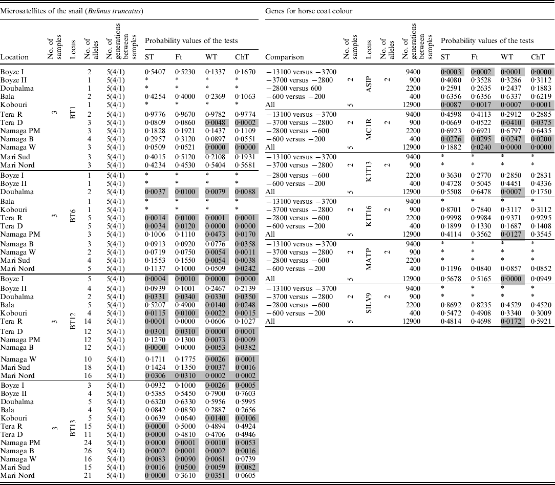
Finally, the four tests were applied to two real datasets: (i) frequencies of four microsatellite loci from the snail Bulinus truncatus (Viard et al., Reference Viard, Justy and Jarne1997) taken at three different times separated by four and one generations, which were obtained from 12 locations, and (ii) frequencies from six sequenced genes (analysed as biallelic systems) that are involved in the expression of the skin colour of horses, dated at 5 times over a 12 900-year period (13 100, 3700, 2800, 600, and 200 BC) reported by Ludwig et al. (Reference Ludwig, Pruvost, Reissmann, Benecke, Brockmann, Castaños, Cieslak, Lippold, Llorente, Malaspinas, Slatkin and Hofreiter2009) (Table 1).
Table 1. Results for the two real data sets analysed. In the snail data set, the numbers under the label ‘No. of generations between samples’ indicate the number of generations between the first and last samples, while the numbers inside the parentheses indicate the generations between consecutive samples. Grey cells indicate significant results (α=0·05), and * indicates analyses that were not possible because of a lack of data or because the locus was monomorphic
(vii) Programming
Multinomial and hypergeometric multivariate deviates were generated by iterative simulation from their univariate marginal densities (Haas & Formery, Reference Haas and Formery2002; Gelman et al., Reference Gelman, Carlin, Stern and Rubin2004), which were obtained with Kemp's (Reference Kemp1986) and Voratas & Schmeiser's (Reference Voratas and Schmeiser1985) methods, respectively. Dirichlet deviates were obtained as explained in Gelman et al. (Reference Gelman, Carlin, Stern and Rubin2004) and in Haas and Formery (Reference Haas and Formery2002) by using the random gamma generator contained in the module ‘random’ (A. Miller, available at: http://www.Mathtools.net). For uniform deviates, the RANLUX module was used (Lüscher, Reference Lüscher1994; James, Reference James1994).
3. Results
(i) Effect of the parameters
After more than 400 ABM simulations were run (lasting more than 2000 h of computer time), the results with the parameters that caused the more pronounced effects are shown below.
For most combinations of the parameters, the ST, F T test, and WT showed small deviations from the expected 5% of the significant tests. However, the ChT gave higher numbers on the significant tests, which apparently increased as the effects of genetic drift accumulated, for the lower population sizes (Fig. 2 A), the higher numbers of generations (Fig. 2 B), or higher numbers of samples (Fig. 2 C and D). Moderate overestimation of the proportion of the significant tests was observed for the WT with small population sizes (<500) (Fig. 2 A), high numbers of generations (Fig. 2 B) or high numbers of samples (Fig. 2 C and D). The proportion of significant tests obtained with the WT was greater than 6% only with very low population sizes (Fig. 2 A) or with numerous samples (>10) (Fig. 2 D). The low-population-sizes departure could be related to a high sample size to effective population size ratios (S/N e) in addition to the small population size effect. The effect of S/N e has been demonstrated by Waples (Reference Waples1989a) and was also detected here in a group of simulations with different S/N e ratios (from 0·1 to 0·9; results not shown). Interestingly, the ChT and WT performed well with high numbers of alleles or loci (not shown), but both showed a higher proportion of significant tests than the ST or F T test.
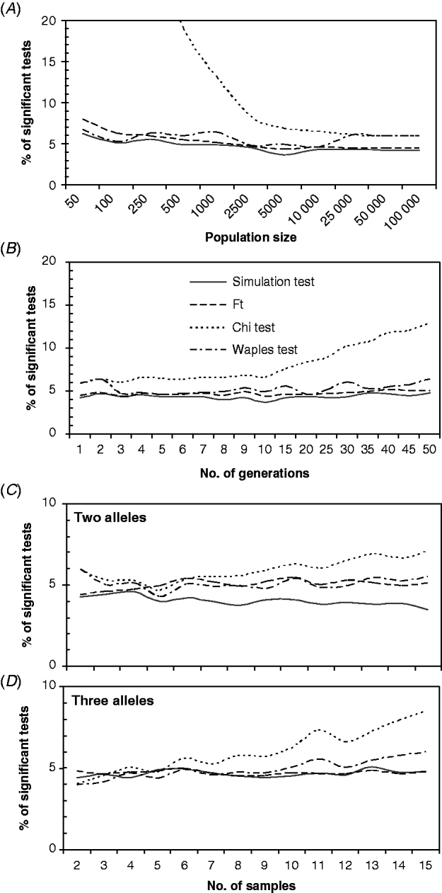
Fig. 2. Percentage of significant tests obtained for different values of: (A) total population sizes (N), (B) numbers of generations between samples; and an increasing number of samples/generations, with two alleles (C) or three alleles (D). The default settings were (unless otherwise is indicated) as follows: N=10 000, N e=N/2, t=5, two samples with sizes S 0=S 5=100, number of alleles k=2, initial allele frequencies of 0·5, sampling Plan II and fully Bayesian algorithm. In (C) and (D), only one generation separated consecutive samples, and the initial allele frequencies were 0·95/0·05 and 0·7/0·28/0·02, respectively.
On the other hand, for the ST and F T test, differences greater than 2% from the expected value of 5% of the significant tests were not observed for most combinations of the parameters, and in general, the proportion of significant tests obtained with these methods was below 5%.
In order to determine whether the small departures from the expected number of significant tests that were found for several parameter ranges were accumulative, a set of ABM simulations was run with ‘problematic’ combinations of parameter values. Figure 3 shows that when many alleles were analysed, with some at very low frequencies, and the samples were increased simultaneously while the population size was reduced, the proportion of significant tests obtained with the ChT rose rapidly to very high values. In addition, the otherwise stable WT yielded a proportion of significant tests that was greater than 10%. The ST and F T test maintained their previously observed stability, giving a proportion of significant tests which was close to 5%.

Fig. 3. The graphics show the percentages of significant values obtained for different numbers of samples and alleles and for three different population sizes, N, as indicated in the graphics. The higher numbers of alleles/samples could not be used with the smaller population sizes (N=100 and 150), because the likelihood of an allele being lost is very high with a large number of alleles and a small number of organisms (the general simulations do not allow samples with missing alleles). The number of samples was the same as the number of alleles for each run. They were increased simultaneously just to assess the combined effect of the parameters in a simple form, because our goal was not to analyse the effect of each parameter (that was already done) but the magnitude the departures can reach with certain ‘problematic’ combinations of parameters. For that purpose, the following settings were used: N e=N/2, one generation between consecutive samples, sample sizes were all the same Si=20, sampling Plan II and fully Bayesian algorithm. The initial allele frequencies were as follows: 0·5/0·5 (two alleles), 0·25/0·25/0·5 (three alleles), 0·167/0·167/0·167/0·5 (four alleles), 0·125/0·125/0·125/0·125/0·5 (five alleles), 0·1/0·1/0·1/0·1/0·1/0·5 (six alleles), 0·083/…/0·083/0·5 (seven alleles), 0·071/…/0·071/0·5 (eight alleles), 0·0625/…/0·0625/0·5 (nine alleles) and 0·055/…/0·055/0·5 (ten alleles).
(ii) Binomial simulation test (bST)
After many combinations of parameters were assayed, the bST presented relevant increases of significant tests with a decreasing number of alleles, a decreasing number of samples, low sample and population sizes, an increasing number of generations and values of S/N e closer to one (not shown). The number of significant tests obtained with the bST reached 15%. In order to inquire into this unexpected result, a set of runs with small population sizes, decreasing sample sizes, different S/N e values as well as different sampling plans were run. Figure 4 displays the differences of the percentage of statistical tests between bST and (hypergeometric) ST, which showed positive values when the binomial version had a higher % and negative when the hypergeometric version had a higher %. The curves corresponding to two different S/N e values and the two sampling plans support that two putative causes explain the binomial test bias: (i) a reduction in the total population and (ii) a negative correlation between population and sample allele frequencies. Both produced the effect of enhancing the differences among the frequencies of the samples when hypergeometric and sampling Plan II was present, making the binomial test to overestimate significant tests by simulating samples with lower differences than the real ones. This effect was present only with a combination of low population sizes, high S/N e values and sampling Plan II (see the complete explanation in section 4).

Fig. 4. Difference between binomial and hypergeometric significant STs, and for tests over the F T statistic. Graphics show the % of the significant tests obtained with binomial ST minus the % obtained with hypergeometric ST, as a function of sample sizes. Two S–N e ratios and sampling plans were used, S/N e=0·9 and S/N e=0·5; and Plan I (before reproduction) and Plan II (after reproduction). Curves correspond to: (A) S/N e=0·9, Plan II; (B) S/N e=0·5, Plan II; (C) S/N e=0·9, Plan I, (D) S/N e=0·5, Plan I. A curve in the positive region meant that the % of significant bSTs was larger than the % of hypergeometric tests, and a curve in the negative region the converse. The default settings were as follows: N=2N e, t=5 (generations between samples), k=2, initial allele frequencies of 0·5/0·5 and fully Bayesian algorithm. Notice that, since N, N e were fixed for each curve, the x-axis not only indicates increasing sample sizes but also increasing N and N e.
(iii) Statistical robustness and power
In the analysis of statistical robustness, as the population size used by the tests was increased with respect to the real population size (ABM simulations), the number of significant tests increased, while a reduction in the sizes used by the tests produced a reduction in the number of significant tests. As expected, the ChT appeared more robust, because it did not require the parameters N and N e (Fig. 5 B and C). The statistical power of the ChT was greater than that of the other tests for a selection coefficient of 1·01, but similar to that of the other tests for higher selection coefficients (Fig. 5 A). The ST, F T test and WT all showed a very similar statistical power to each other with each of the three different selection coefficients used.

Fig. 5. (A) Percentage of significant tests obtained when the frequency of one allele in the ‘real population’ (the ABM simulation) was increased by a given amount (s=1·01×, 1·05× and 1·1×) each generation, emulating a positive selection process. (B, C) Percentage of significant tests when incorrect values of N were used by the tests (x-axis) for two different values of real population size (the used in general simulations): N=1000 (B) and N=10 000 (C). The default parameters used were as follows: N=10 000, N e=N/2, t=5, S 0=S 5=100, number of alleles k=2, initial allele frequencies of 0·5, sampling Plan II and full Bayesian algorithm.
(iv) Real data sets
Table 1 shows the results for the two real data sets. In the data set of the snail B. truncatus, from 41 tests on microsatellite loci that contained between 2 and 26 alleles, around 12 presented quite different probability values among the tests. The loci with large differences (among the tests) were mostly the ones with many alleles at very low frequencies. ST and F T tended to present higher values of probability than WT and ChT.
In the genes data set for equine colour coat, ST and F T were found to tend to yield higher probabilities than WT and ChT. From the 17 tests applied, two showed significant results for all tests, and one was significant for WT and ChT (P~0·04) but not with the ST and F T (P~0·06). The overall tests with all the samples involved simultaneously showed low probabilities with WT or ChT in five (from six) loci, while the same loci showed high probabilities (>0·2) with ST and F T. The most relevant differences were found among tests that attained very low-frequency alleles.
4. Discussion
The observed deviations of the ChT from the expected value of 5% of the significant tests (with almost all the parameters assayed) can be explained mainly by the effect of genetic drift, as pointed out by Waples (Reference Waples1989a) . Here, low population sizes, high numbers of samples and generations between samples produced an extremely high number of false significant tests with the ChT.
Contrastingly, the ST, F T test and WT performed homogeneously, showing low to moderate deviations from the expected value. The differences were larger for the smaller population sizes, higher number of samples and higher number of loci. These deviations had different origins.
The deviations that were obtained with the WT for small population sizes may have originated in the departure of the statistic used from a χ2 distribution, already identified by Goldringer & Bataillon (Reference Goldringer and Bataillon2004) who suggested the simulation-generated distribution of the Fc,l statistic as the basis of a test for assaying temporal changes. The effect of small population sizes, together with large sample sizes, has already been recognized as an analytical problem that produces errors in the estimation of effective population size by the temporal method (Nei & Tajima, Reference Nei and Tajima1981; Pollak, Reference Pollak1983; Waples, Reference Waples1989b). However, a component of this bias could be the effect of the S/N e ratio demonstrated by Waples (Reference Waples1989a) and others that increase as population sizes decrease for constant sample sizes, and that could be related to the increased statistical power of samples proportionally larger with respect to the effective population size. In spite of non-replacement (hypergeometric) samples having a smaller variance than replacement (binomial) samples, it is expected that an underestimation of significant tests with the bST but not with the WT since the sampling used by Waples (Reference Waples1989a, Reference Waplesb) refers to the previous generation and those differences are not expected to affect the results of the test, as actually happened. However, in runs with small population sizes and sample sizes similar to N e (S/N e~1·0), the bST not only underestimated the % of the significant tests, but also presented important overestimations of those percentages. This was caused by the use of sampling Plan II over most of the simulations of the study since this plan's results were more realistic. With this scenario (small N and S/N e~1·0), two effects would enhance differences among allele frequencies at temporally spaced samples in a real population (with hypergeometric-like sampling): (i) since the sampling would be proportionally large and the population size small, the sampled alleles would leave the population with a size even smaller and consequently more susceptible to changes by drift and (ii) with such a small population size and proportionally large sample size, the allele frequencies in the sample and in the population (after sampling) would establish a trade-off. For instance, in a population with an allele at a frequency of 0·5 before sampling, if N were so small that S=N/2 is true, then the frequency of the allele of 0·7 in the sample would mean a frequency in the population of 0·3; that is, the higher the number of alleles in the first sample, the lower the remaining in the population and thus at posterior samples. Both effects are absent from binomial simulations since (i) a constraint in binomial distribution prevents programming the discounting of sampled alleles from the total population (e.g. the binomial sample could actually have more alleles of one type than the original number of alleles in the population, and so the frequency in the population after discounting the sample would be negative!) and (ii) since the alleles sampled binomially are sampled with replacement, the frequencies cannot establish a trade-off with the frequencies in the population.
Those mechanisms explain that under small population sizes, S/N e~1·0, and sampling Plan II, the hypergeometric simulations as well as the real populations should present higher differences in allele frequencies among the samples than binomial simulations. Thus, for fixed (observed) frequencies, the binomial test generates fewer simulations with differences equal or higher than the observed ones, underestimating the P-values and thus overestimating the % of the significant tests. The results shown in Fig. 4 support the explained mechanisms with three facts: (i) the curves had lower values for higher sample sizes, which meant not higher S/N e but higher population sizes, i.e. for higher population sizes, the binomial bias was lost; (ii) the curves with S/N e=0·5 had lower values than with S/N e=1·0, i.e. the binomial bias became weaker as the sample sizes became lower than the population sizes and (iii) the curves obtained with sampling Plan I returned to negative values when the sample sizes (i.e. the population sizes) increased, which means that in the absence of sampling Plan II the binomial bias could be inverted, and the differences would be caused by the mentioned difference between hypergeometric and binomial variances.
Thus, the Waples test, the Goldringer and Bataillon test and other binomial sampling-based tests potentially would have two sources of bias with opposite effects: the difference between the hypergeometric and binomial variances and the one explained above.
Furthermore, the WT and binomial bias observed for the increased number of generations and samples could be related to the assumption that the model of F (the standardized temporal variance in allele frequencies) has to be proportional to t/2N e which becomes particularly relevant at large t and very small N e values (Waples, Reference Waples1989a, Reference Waplesb).
The results of the analysis of the real data sets agreed with the ABM simulation results. In the case of the snail, B. truncatus, the largest differences among ST/F T and WT/ChT were found in loci with many alleles from which several had low frequencies. In addition, the study attained low population sizes (N=1000) and three samples. All these factors brought the studied system closer to that represented by the ‘problematic’ combinations of parameters that were assayed with the ABM simulations, where the WT and ChT gave smaller P-values, in agreement with the tendency of WT and ChT to yield lower P-values than ST and F T in the snail data set.
In addition, the second real data set analysed the frequencies of genes for horse coat colour had features similar to the problematic combinations, such as having a very large number of generations among samples, many samples and low-frequency alleles. They also showed a similar tendency: lower P-values with WT and ChT than with ST and F T.
The possible explanation for the behaviour observed with problematic combinations is probably composed. Some components could be the mentioned departures of the χ2 distribution or the binomial-hypergeometric bias(es). Another relevant component is a boundary effect of low initial allele frequencies. Additional simulations were performed to probe the effect of low allele frequencies and showed a tendency to yield increased probability values, which were larger with the ST. The boundary conditions already detected by Waples (Reference Waples1989a) involved a large probability that the allele detected was lost. Such a loss would prevent further change in the allele frequency, reducing the possibility of a type II error (Liukart et al., Reference Liukart, Cornuet and Allendorf1999; Goldringer & Bataillon, Reference Goldringer and Bataillon2004).
Another interesting and unexpected result was found with the snail data set. Five loci presented substantially larger probability values with the ChT and WT than with the ST and F T test. These loci all corresponded to a high number of alleles, many of which had very low frequencies, and some alleles had been lost in one or more samples. One hypothesis to explain this phenomenon is that the absence of an allele in some samples, in conjunction with its occurrence at a high frequency in another sample, will occur very infrequently by chance alone, due to the mentioned boundary effect. Thus, the STs (ST and FT), as real populations, were reluctant to allow alleles at very low frequencies arising suddenly by chance, whereas ChT and WT summarize the overall differences among alleles and samples without discriminating among common patterns or very improbable patterns (e.g. absence/presence-at-high- frequency/absence of an allele). Additional (ABM) simulations with the selection-like process acting on low-frequency alleles supported this statement.
In addition, the ST, F T test and WT showed similar statistical robustness and statistical power, which precluded the possibility that the differences observed with the snail data were due to the effect of differential statistical powers for the tests, and not to population sizes.
Finally, it can be said that the WT, ST and F T test performed better than the ChT, as expected, because they took into account the effect of genetic drift. However, for certain combinations of parameters, the ST and F T test yielded more reliable results, which makes them more suitable for studies that involve many samples, low population sizes and high numbers of alleles (as in the case of microsatellite or sequence data). Further studies are required to explore the combined effect of small population sizes, multiple alleles and samples, S/N e, together with the effect of having low-frequency alleles.
Software implementing the described tests is available at: http://sites.google.com/site/egenevol/home or from esandoval@miranda.ecologia.unam.mx by request.
I thank Manuel Uribe-Alcocer, Lourdes Barbosa-Saldaña, Luis Medrano-González, Robin Waples, and two anonymous reviewers for their comments on earlier versions of this paper.


