


1 Introduction
The Virasoro constraints are a conjecture in Gromov–Witten theory, proposed by Eguchi, Hori and Xiong [Reference Eguchi, Hori and Xiong5] for any smooth projective complex variety Y with only $(p,p)$
-cohomology. S. Katz helped to establish a general conjecture. We review the conjecture below. The Virasoro constraints have been proven if Y is a toric threefold; see [Reference Givental8]. Recently, Moreira, Oblomkov, Okounkov and Pandharipande [Reference Moreira, Oblomkov, Okounkov and Pandharipande21] used the Gromov–Witten/Pandharipande–Thomas (GW/PT) correspondence [Reference Pandharipande and Pixton25, Reference Pandharipande and Pixton28, Reference Pandharipande and Pixton27, Reference Pandharipande and Pixton29] to obtain constraints on the moduli space of stable pairs of a toric 3-fold. In [Reference Moreira, Oblomkov, Okounkov and Pandharipande21] and [Reference Moreira20], the theory was applied to the case where the toric 3-fold is
$(p,p)$
-cohomology. S. Katz helped to establish a general conjecture. We review the conjecture below. The Virasoro constraints have been proven if Y is a toric threefold; see [Reference Givental8]. Recently, Moreira, Oblomkov, Okounkov and Pandharipande [Reference Moreira, Oblomkov, Okounkov and Pandharipande21] used the Gromov–Witten/Pandharipande–Thomas (GW/PT) correspondence [Reference Pandharipande and Pixton25, Reference Pandharipande and Pixton28, Reference Pandharipande and Pixton27, Reference Pandharipande and Pixton29] to obtain constraints on the moduli space of stable pairs of a toric 3-fold. In [Reference Moreira, Oblomkov, Okounkov and Pandharipande21] and [Reference Moreira20], the theory was applied to the case where the toric 3-fold is $X \times \mathbb {P}^1$
, for X a toric surface. In the second reference, a cobordism argument is used to prove constraints for the Hilbert scheme of points of X for any simply connected surface X. In this paper, we conjecture Virasoro constraints extending this result to moduli spaces of sheaves of rank
$X \times \mathbb {P}^1$
, for X a toric surface. In the second reference, a cobordism argument is used to prove constraints for the Hilbert scheme of points of X for any simply connected surface X. In this paper, we conjecture Virasoro constraints extending this result to moduli spaces of sheaves of rank $r \geq 1$
. In doing so, we address a question of R. Pandharipande, who asked in his Hangzhou lecture on Virasoro constraints (April 2020) whether the moduli space of stable sheaves admits such constraints.
$r \geq 1$
. In doing so, we address a question of R. Pandharipande, who asked in his Hangzhou lecture on Virasoro constraints (April 2020) whether the moduli space of stable sheaves admits such constraints.
1.1 Virasoro constraints in GW-theory
We review the Virasoro conjecture for GW-theory. For a more complete exposition, we refer to [Reference Pandharipande24, Sec. 4] or [Reference Moreira, Oblomkov, Okounkov and Pandharipande21]. Let Y be a smooth projective complex variety. Assume for simplicity that Y has only $(p,p)$
-cohomology. For any nonnegative numbers n, g and any
$(p,p)$
-cohomology. For any nonnegative numbers n, g and any $\beta \in H_2(Y, \mathbb {Z})$
, we associate to Y the moduli space of stable maps
$\beta \in H_2(Y, \mathbb {Z})$
, we associate to Y the moduli space of stable maps $\bar {M}_{g, n}(Y, \beta )$
. Recall that a stable map is a morphism
$\bar {M}_{g, n}(Y, \beta )$
. Recall that a stable map is a morphism $f : C \to Y$
, where C is a connected genus g curve with at most nodal singularities and n marked smooth points
$f : C \to Y$
, where C is a connected genus g curve with at most nodal singularities and n marked smooth points $x_1, x_2, \ldots , x_n$
. Furthermore, f should satisfy
$x_1, x_2, \ldots , x_n$
. Furthermore, f should satisfy $f_*[C] = \beta $
. Then there are canonical maps
$f_*[C] = \beta $
. Then there are canonical maps $\operatorname {\mathrm {ev}}_i : \bar {M}_{g,n}(Y, \beta ) \to Y$
which send a stable map
$\operatorname {\mathrm {ev}}_i : \bar {M}_{g,n}(Y, \beta ) \to Y$
which send a stable map $(C, f)$
to
$(C, f)$
to $f(x_i)$
, the image of the i-th marked point. Also,
$f(x_i)$
, the image of the i-th marked point. Also, $\bar {M}_{g,n}(Y, \beta )$
admits n canonical line bundles
$\bar {M}_{g,n}(Y, \beta )$
admits n canonical line bundles $M_i$
for
$M_i$
for $1 \leq i \leq n$
. At the point
$1 \leq i \leq n$
. At the point $(C, f)$
,
$(C, f)$
, $M_i$
is the cotangent bundle to C at
$M_i$
is the cotangent bundle to C at $x_i$
. Then we define the descendant GW-invariants as
$x_i$
. Then we define the descendant GW-invariants as
 $$ \begin{align*} \langle \tau_{k_1}(\gamma_1) \tau_{k_2}(\gamma_2) \ldots \tau_{k_n}(\gamma_n)\rangle^Y_{g,\beta} = \int_{[\bar{M}_{g,n}(Y, \beta)]^{\text{vir}}} c_1(M_1)^{k_1}\operatorname{\mathrm{ev}}_1^*(\gamma_1) \cdots c_1(M_n)^{k_n} \operatorname{\mathrm{ev}}_n^*(\gamma_n). \end{align*} $$
Now, fix a basis $\{\gamma _i\}_{i = 1,\ldots ,r}$
of
$\{\gamma _i\}_{i = 1,\ldots ,r}$
of $H^\bullet (Y, \mathbb {Q})$
, which is homogeneous with respect to the degree decomposition. Let
$H^\bullet (Y, \mathbb {Q})$
, which is homogeneous with respect to the degree decomposition. Let $\lambda $
, q and
$\lambda $
, q and $\{t^a_k\}_{k = 0,1,\ldots }^{a = 1,\ldots ,r}$
be formal variables. Then we define the GW-partition function as
$\{t^a_k\}_{k = 0,1,\ldots }^{a = 1,\ldots ,r}$
be formal variables. Then we define the GW-partition function as
 $$ \begin{align*} F^Y = \sum_{g\geq 0} \lambda^{2g-2} \sum_{\beta \in H_2(Y, \mathbb{Z})} q^\beta \sum_{n \geq 0} \frac{1}{n!} \sum_{\substack{a_1,\ldots,a_n \\ k_1,\ldots,k_n}} t^{a_1}_{k_1}\cdots t^{a_n}_{k_n} \langle \tau_{k_1}(\gamma_{a_1}) \ldots \tau_{k_n}(\gamma_{a_n}) \rangle^X_{g, \beta.} \end{align*} $$
Let $Z^Y = \exp (F^Y)$
. The Virasoro conjecture states that
$Z^Y = \exp (F^Y)$
. The Virasoro conjecture states that $L^{\text {GW}}_k(Z^Y) = 0$
, where
$L^{\text {GW}}_k(Z^Y) = 0$
, where $L^{\text {GW}}_k$
are certain formal differential operators defined for
$L^{\text {GW}}_k$
are certain formal differential operators defined for $k\geq -1$
. We will not give the formulae for the
$k\geq -1$
. We will not give the formulae for the $L_k^{\text {GW}}$
here; see [Reference Pandharipande24, Sec. 4] for those. The operators
$L_k^{\text {GW}}$
here; see [Reference Pandharipande24, Sec. 4] for those. The operators $L_k^{\text {GW}}$
are called the Virasoro operators, and they satisfy the Virasoro bracket
$L_k^{\text {GW}}$
are called the Virasoro operators, and they satisfy the Virasoro bracket
 $$ \begin{align} [L^{\text{GW}}_k, L^{\text{GW}}_n] = (n - k)L^{\text{GW}}_{k+n}. \end{align} $$
The Virasoro conjecture expresses relations among integrals in $\bar {M}_{g,n}(Y, \beta )$
for various g, n and
$\bar {M}_{g,n}(Y, \beta )$
for various g, n and $\beta $
. It is possible to write these relations rather explicitly. Let
$\beta $
. It is possible to write these relations rather explicitly. Let $\mathbb {D}^Y_{\text {GW}}$
be the commutative
$\mathbb {D}^Y_{\text {GW}}$
be the commutative $\mathbb {Q}$
-algebra generated by formal symbols
$\mathbb {Q}$
-algebra generated by formal symbols $\tau _k(\gamma _i)$
. Then one can define certain operators
$\tau _k(\gamma _i)$
. Then one can define certain operators $\mathcal {L}_k^{\text {GW}}$
on this algebra for
$\mathcal {L}_k^{\text {GW}}$
on this algebra for $k \geq -1$
which satisfy the Virasoro bracket. Then it is possible to formulate the Virasoro constraints as
$k \geq -1$
which satisfy the Virasoro bracket. Then it is possible to formulate the Virasoro constraints as
 $$ \begin{align*} \big\langle \mathcal{L}_k^{\text{GW}}(D) \big\rangle^{Y, \bullet}_\beta = 0. \end{align*} $$
This should hold for all $k \geq -1$
and
$k \geq -1$
and $D \in \mathbb {D}_{\text {GW}}^Y$
. Here,
$D \in \mathbb {D}_{\text {GW}}^Y$
. Here, $\langle - \rangle ^{Y, \bullet }_{\beta }$
denotes a certain generating series defined for all elements of
$\langle - \rangle ^{Y, \bullet }_{\beta }$
denotes a certain generating series defined for all elements of $\mathbb {D}^Y_{\text {GW}}$
; see [Reference Moreira, Oblomkov, Okounkov and Pandharipande21] for a definition. This formulation of the Virasoro constraints generalises to other contexts, as we will see below.
$\mathbb {D}^Y_{\text {GW}}$
; see [Reference Moreira, Oblomkov, Okounkov and Pandharipande21] for a definition. This formulation of the Virasoro constraints generalises to other contexts, as we will see below.
1.2 Virasoro constraints for stable pairs
Recall that a stable pair on a smooth projective threefold Y is a map of coherent sheaves $s : \mathcal {O}_Y \to F$
such that F is pure of dimension 1 (i.e., every nonzero subsheaf of F has dimension 1) and
$s : \mathcal {O}_Y \to F$
such that F is pure of dimension 1 (i.e., every nonzero subsheaf of F has dimension 1) and $\dim \operatorname {\mathrm {Supp}} \operatorname {\mathrm {coker}} s = 0$
. Associated to such a pair are two invariants,
$\dim \operatorname {\mathrm {Supp}} \operatorname {\mathrm {coker}} s = 0$
. Associated to such a pair are two invariants, $n = \chi (Y, F)$
and
$n = \chi (Y, F)$
and $\beta \in H_2(Y, \mathbb {Z})$
, the homology class associated to
$\beta \in H_2(Y, \mathbb {Z})$
, the homology class associated to $\operatorname {\mathrm {Supp}} F$
. There is a fine projective moduli space
$\operatorname {\mathrm {Supp}} F$
. There is a fine projective moduli space $P = P_n(Y, \beta )$
parametrising stable pairs with these invariants. It carries a virtual fundamental class, and its virtual dimension is
$P = P_n(Y, \beta )$
parametrising stable pairs with these invariants. It carries a virtual fundamental class, and its virtual dimension is $\int _{\beta }c_1(X)$
. See [Reference Pandharipande and Thomas26] for more details.
$\int _{\beta }c_1(X)$
. See [Reference Pandharipande and Thomas26] for more details.
The GW/PT correspondence describes a relationship between the GW- and PT-invariants of a smooth projective threefold. The so-called stationary variant has been proven in the toric case [Reference Pandharipande and Pixton29]. In [Reference Moreira, Oblomkov, Okounkov and Pandharipande21], this correspondence has been made more explicit and it is used to derive constraints for the moduli space of stable pairs on Y.
Define $\mathbb {D}^Y$
to be the
$\mathbb {D}^Y$
to be the $\mathbb {Q}$
-algebra generated by formal symbols
$\mathbb {Q}$
-algebra generated by formal symbols $\operatorname {\mathrm {ch}}_i(\gamma )$
, where
$\operatorname {\mathrm {ch}}_i(\gamma )$
, where $\gamma \in H^\bullet (Y, \mathbb {Q})$
. We impose the relations
$\gamma \in H^\bullet (Y, \mathbb {Q})$
. We impose the relations $\operatorname {\mathrm {ch}}_i(\gamma + \gamma ') = \operatorname {\mathrm {ch}}_i(\gamma ) + \operatorname {\mathrm {ch}}_i(\gamma ')$
and
$\operatorname {\mathrm {ch}}_i(\gamma + \gamma ') = \operatorname {\mathrm {ch}}_i(\gamma ) + \operatorname {\mathrm {ch}}_i(\gamma ')$
and $\operatorname {\mathrm {ch}}_i(\lambda \gamma ) = \lambda \operatorname {\mathrm {ch}}_i(\gamma )$
. Again, it is possible to define operators
$\operatorname {\mathrm {ch}}_i(\lambda \gamma ) = \lambda \operatorname {\mathrm {ch}}_i(\gamma )$
. Again, it is possible to define operators $\mathcal {L}_k^{\text {PT}}$
on this algebra. These satisfy the Virasoro bracket in a slightly weaker sense. Fix a number n and a class
$\mathcal {L}_k^{\text {PT}}$
on this algebra. These satisfy the Virasoro bracket in a slightly weaker sense. Fix a number n and a class $\beta \in H_2(Y, \mathbb {Z})$
. Let
$\beta \in H_2(Y, \mathbb {Z})$
. Let $P = P_n(Y, \beta )$
be the moduli space of stable pairs. Then there is an algebra homomorphism
$P = P_n(Y, \beta )$
be the moduli space of stable pairs. Then there is an algebra homomorphism $\mathbb {D}^Y \to H^\bullet (P, \mathbb {Q})$
by sending
$\mathbb {D}^Y \to H^\bullet (P, \mathbb {Q})$
by sending $\operatorname {\mathrm {ch}}_i(\gamma )$
to
$\operatorname {\mathrm {ch}}_i(\gamma )$
to
 $$ \begin{align*} \pi_{P, *}(\operatorname{\mathrm{ch}}_i(\mathbb{F} - \mathcal{O}_{Y \times P}) \cdot \pi^*_Y(\gamma)). \end{align*} $$
Here, $\pi _P$
and
$\pi _P$
and $\pi _Y$
are the projection from
$\pi _Y$
are the projection from $Y \times P$
to P and Y, respectively, and
$Y \times P$
to P and Y, respectively, and $\mathcal {O}_{Y \times P} \to \mathbb {F}$
is the universal stable pair on
$\mathcal {O}_{Y \times P} \to \mathbb {F}$
is the universal stable pair on $Y \times P$
. The Virasoro constraints obtained by [Reference Moreira, Oblomkov, Okounkov and Pandharipande21] can now be expressed as
$Y \times P$
. The Virasoro constraints obtained by [Reference Moreira, Oblomkov, Okounkov and Pandharipande21] can now be expressed as
 $$ \begin{align*} \int_{[P_n(Y, \beta)]^{\text{vir}}} \mathcal{L}_k^{\text{PT}}D = 0 \end{align*} $$
for all $D \in \mathbb {D}^Y$
and all
$D \in \mathbb {D}^Y$
and all $k \geq -1$
. (Here, the map to the cohomology of P is left implicit.) These constraints have been proven for Y toric, if D is contained in a certain subalgebra of
$k \geq -1$
. (Here, the map to the cohomology of P is left implicit.) These constraints have been proven for Y toric, if D is contained in a certain subalgebra of $\mathbb {D}^Y$
consisting of the stationary invariants (see [Reference Moreira, Oblomkov, Okounkov and Pandharipande21, Thm. 4]).
$\mathbb {D}^Y$
consisting of the stationary invariants (see [Reference Moreira, Oblomkov, Okounkov and Pandharipande21, Thm. 4]).
Note that in contrast to the Gromov–Witten case, here we have relations between integrals on a single moduli space. We did not write out the formula for $\mathcal {L}_k^{\text {PT}}$
, but it is very similar to our Definition 1.2, and the reader is encouraged to compare our definition with Definition 2 in [Reference Moreira, Oblomkov, Okounkov and Pandharipande21].
$\mathcal {L}_k^{\text {PT}}$
, but it is very similar to our Definition 1.2, and the reader is encouraged to compare our definition with Definition 2 in [Reference Moreira, Oblomkov, Okounkov and Pandharipande21].
1.3 Virasoro constraints for the Hilbert scheme
In [Reference Moreira, Oblomkov, Okounkov and Pandharipande21, Sec. 6] they take $Y = X \times \mathbb {P}^1$
, for X a toric surface. If one takes any
$Y = X \times \mathbb {P}^1$
, for X a toric surface. If one takes any $x \in X$
, then the moduli space of pairs
$x \in X$
, then the moduli space of pairs $P_n(X \times \mathbb {P}^1, n[\{x\} \times \mathbb {P}^1])$
is canonically isomorphic to
$P_n(X \times \mathbb {P}^1, n[\{x\} \times \mathbb {P}^1])$
is canonically isomorphic to $\operatorname {\mathrm {Hilb}}^n(X)$
. The Virasoro constraints of pairs induce constraints on
$\operatorname {\mathrm {Hilb}}^n(X)$
. The Virasoro constraints of pairs induce constraints on $\operatorname {\mathrm {Hilb}}^n(X)$
. We have the algebra
$\operatorname {\mathrm {Hilb}}^n(X)$
. We have the algebra $\mathbb {D}^X$
, which is defined in the same way as before. We have an operator
$\mathbb {D}^X$
, which is defined in the same way as before. We have an operator $\mathcal {L}_k$
, which is the same as the one from Definition 1.2. We also have a ring homomorphism
$\mathcal {L}_k$
, which is the same as the one from Definition 1.2. We also have a ring homomorphism $\mathbb {D}^X \to H^\bullet (\operatorname {\mathrm {Hilb}}^n(X), \mathbb {Q})$
, which is defined by sending
$\mathbb {D}^X \to H^\bullet (\operatorname {\mathrm {Hilb}}^n(X), \mathbb {Q})$
, which is defined by sending $\operatorname {\mathrm {ch}}_i(\gamma )$
to
$\operatorname {\mathrm {ch}}_i(\gamma )$
to
 $$ \begin{align*} \pi_{\operatorname{\mathrm{Hilb}}^n(X), *}(-\operatorname{\mathrm{ch}}_k(\mathcal{I}) \cdot \pi_X^*(\gamma)), \end{align*} $$
where $\pi _{\operatorname {\mathrm {Hilb}}_n(X)}$
and
$\pi _{\operatorname {\mathrm {Hilb}}_n(X)}$
and $\pi _X$
are the projections from
$\pi _X$
are the projections from $X \times \operatorname {\mathrm {Hilb}}^n(X)$
to
$X \times \operatorname {\mathrm {Hilb}}^n(X)$
to $\operatorname {\mathrm {Hilb}}^n(X)$
and X respectively, and
$\operatorname {\mathrm {Hilb}}^n(X)$
and X respectively, and $\mathcal {I}$
is the universal ideal sheaf. Then the Virasoro constraints are
$\mathcal {I}$
is the universal ideal sheaf. Then the Virasoro constraints are
 $$ \begin{align*} \int_{\operatorname{\mathrm{Hilb}}^n(X)} \mathcal{L}_kD = 0 \end{align*} $$
for all $D \in \mathbb {D}^X$
and all
$D \in \mathbb {D}^X$
and all $k \geq -1$
. This was proven for all smooth projective toric surfaces X in [Reference Moreira, Oblomkov, Okounkov and Pandharipande21, Sec. 6]. In [Reference Moreira20], a similar formula is proven for all simply connected smooth projective surfaces X, using a cobordism argument. This required a modification of the operator
$k \geq -1$
. This was proven for all smooth projective toric surfaces X in [Reference Moreira, Oblomkov, Okounkov and Pandharipande21, Sec. 6]. In [Reference Moreira20], a similar formula is proven for all simply connected smooth projective surfaces X, using a cobordism argument. This required a modification of the operator $\mathcal {L}_k$
because the formula of Definition 1.2 is only correct if X has only
$\mathcal {L}_k$
because the formula of Definition 1.2 is only correct if X has only $(p,p)$
-cohomology.
$(p,p)$
-cohomology.
1.4 Formulation of the conjecture
We will now formulate the main conjecture of this paper. Let X be a surfaceFootnote
1
which only has $(p,p)$
-cohomology and fixed polarisation H. Then
$(p,p)$
-cohomology and fixed polarisation H. Then $H^\bullet (X, \mathbb {Q})= \bigoplus _{i = 0}^2 H^{2i}(X, \mathbb {Q})$
and we refer to the elements of
$H^\bullet (X, \mathbb {Q})= \bigoplus _{i = 0}^2 H^{2i}(X, \mathbb {Q})$
and we refer to the elements of $H^{2i}(X, \mathbb {Q})$
as the cohomology classes of (complex) degree i. We fix in advance integers
$H^{2i}(X, \mathbb {Q})$
as the cohomology classes of (complex) degree i. We fix in advance integers $r> 0$
and
$r> 0$
and $c_2$
and a line bundle
$c_2$
and a line bundle $\Delta $
on X, and we let
$\Delta $
on X, and we let $M = M^H_X(r, \Delta , c_2)$
be the moduli space of Gieseker semistable sheaves (with respect to H) with rank r, determinant
$M = M^H_X(r, \Delta , c_2)$
be the moduli space of Gieseker semistable sheaves (with respect to H) with rank r, determinant $\Delta $
and second Chern class
$\Delta $
and second Chern class $c_2$
.
$c_2$
.
Definition 1.1. We define $\mathbb {D}^X$
as the commutative
$\mathbb {D}^X$
as the commutative $\mathbb {Q}$
-algebra generated by symbols of the form
$\mathbb {Q}$
-algebra generated by symbols of the form $\operatorname {\mathrm {ch}}_i(\gamma )$
, where i is a nonnegative integer and
$\operatorname {\mathrm {ch}}_i(\gamma )$
, where i is a nonnegative integer and $\gamma \in H^\bullet (X, \mathbb {Q})$
. We impose the relations
$\gamma \in H^\bullet (X, \mathbb {Q})$
. We impose the relations $\operatorname {\mathrm {ch}}_i(\gamma _1 + \gamma _2) = \operatorname {\mathrm {ch}}_i(\gamma _1) + \operatorname {\mathrm {ch}}_i(\gamma _2)$
and
$\operatorname {\mathrm {ch}}_i(\gamma _1 + \gamma _2) = \operatorname {\mathrm {ch}}_i(\gamma _1) + \operatorname {\mathrm {ch}}_i(\gamma _2)$
and $\operatorname {\mathrm {ch}}_i(\lambda \cdot \gamma ) = \lambda \cdot \operatorname {\mathrm {ch}}_i(\gamma )$
. We define a grading on
$\operatorname {\mathrm {ch}}_i(\lambda \cdot \gamma ) = \lambda \cdot \operatorname {\mathrm {ch}}_i(\gamma )$
. We define a grading on $\mathbb {D}^X$
by declaring that the degree of
$\mathbb {D}^X$
by declaring that the degree of $\operatorname {\mathrm {ch}}_i(\gamma )$
is
$\operatorname {\mathrm {ch}}_i(\gamma )$
is $i + \deg \gamma - 2$
.
$i + \deg \gamma - 2$
.
Later, we will interpret the $\operatorname {\mathrm {ch}}_i(\gamma )$
’s as elements of the cohomology on M. The degree of
$\operatorname {\mathrm {ch}}_i(\gamma )$
’s as elements of the cohomology on M. The degree of $\operatorname {\mathrm {ch}}_i(\gamma )$
is chosen so that it matches the degree of the cohomology class we will associate to it. We introduce
$\operatorname {\mathrm {ch}}_i(\gamma )$
is chosen so that it matches the degree of the cohomology class we will associate to it. We introduce $\mathbb {D}^X$
because the operator
$\mathbb {D}^X$
because the operator $\mathcal {L}_k$
defined below does not descend to the level of cohomology. The next definition extends the one given in [Reference Moreira, Oblomkov, Okounkov and Pandharipande21] and [Reference Moreira20].Footnote
2
$\mathcal {L}_k$
defined below does not descend to the level of cohomology. The next definition extends the one given in [Reference Moreira, Oblomkov, Okounkov and Pandharipande21] and [Reference Moreira20].Footnote
2
Definition 1.2. For each $k \geq -1$
, we define an operator
$k \geq -1$
, we define an operator $\mathcal {L}_k$
on
$\mathcal {L}_k$
on $\mathbb {D}^X$
as
$\mathbb {D}^X$
as $R_k + T_k + S_k$
, where the latter three operators are:
$R_k + T_k + S_k$
, where the latter three operators are:
-
○ $R_k$
is defined by
$R_k\operatorname {\mathrm {ch}}_i(\gamma ) = \prod _{j = 0}^k (i + j + d - 2) \operatorname {\mathrm {ch}}_{i + k}(\gamma )$
for
$\gamma \in H^\bullet (X, \mathbb {Q})$
of degree d. We then define it on all of
$\mathbb {D}^X$
by requiring it to be a derivation. In particular,
$R_{-1}\operatorname {\mathrm {ch}}_i(\gamma ) = \operatorname {\mathrm {ch}}_{i - 1}(\gamma )$
, where we agree that
$\operatorname {\mathrm {ch}}_{-1}(\gamma ) = 0$
.
$R_k$
is defined by
$R_k\operatorname {\mathrm {ch}}_i(\gamma ) = \prod _{j = 0}^k (i + j + d - 2) \operatorname {\mathrm {ch}}_{i + k}(\gamma )$
for
$\gamma \in H^\bullet (X, \mathbb {Q})$
of degree d. We then define it on all of
$\mathbb {D}^X$
by requiring it to be a derivation. In particular,
$R_{-1}\operatorname {\mathrm {ch}}_i(\gamma ) = \operatorname {\mathrm {ch}}_{i - 1}(\gamma )$
, where we agree that
$\operatorname {\mathrm {ch}}_{-1}(\gamma ) = 0$
. -
○
$T_k$
is multiplication by a fixed element of
$\mathbb {D}^X$
, namely (2)Here, we are using
$$ \begin{align} T_k = & - \sum_{a + b = k + 2} (-1)^{(d^L + 1)(d^R + 1)}(a + d^L - 2)!(b + d^R - 2)!\operatorname{\mathrm{ch}}_a\operatorname{\mathrm{ch}}_b(1)\\ &+ \sum_{a + b = k} a!b!\operatorname{\mathrm{ch}}_a\operatorname{\mathrm{ch}}_b\bigg(\frac{c_1(X)^2 + c_2(X)}{12}\bigg) \nonumber. \end{align} $$
as an abbreviation for
$$ \begin{align*}(-1)^{(d^L + 1)(d^R + 1)}(a + d^L - 2)!(b + d^R - 2)!\operatorname{\mathrm{ch}}_a\operatorname{\mathrm{ch}}_b(1)\end{align*} $$
where
$$ \begin{align*}\sum_i (-1)^{(\deg(\gamma_i^L) + 1)(\deg(\gamma_i^R) + 1)}(a + \deg(\gamma_i^L) - 2)!(b + \deg(\gamma_i^R) - 2)!\operatorname{\mathrm{ch}}_a(\gamma_i^L)\operatorname{\mathrm{ch}}_b(\gamma_i^R),\end{align*} $$
$\sum _i \gamma _i^L \otimes \gamma _i^R$
is the Künneth decomposition of
$\Delta _*1 \in H^4(X \times X,\mathbb {Q})$
. In the second sum,
$\operatorname {\mathrm {ch}}_a\operatorname {\mathrm {ch}}_b\Big(\frac {c_1(X)^2 + c_2(X)}{12}\Big )$
is a similar abbreviation. Note that on X we have an equality
$\frac {c_1(X)^2 + c_2(X)}{12} = \chi (X, \mathcal {O}_X) \cdot \mathbf {p}$
by Hirzebruch–Riemann–Roch, where
$\mathbf {p}$
is the point class. Finally, we adopt the convention that factorials of negative numbers are zero.
-
○
$S_k$
is defined by setting
$S_kD = \frac {(k+1)!}{r} R_{-1}(\operatorname {\mathrm {ch}}_{k+1}(\mathbf {p})D)$
. Here,
$\mathbf {p} \in H^4(X, \mathbb {Q})$
again corresponds to the class of a point.


Note that the definition of $S_k$
depends on the rank r, but the definition of
$S_k$
depends on the rank r, but the definition of $R_k$
and
$R_k$
and $T_k$
do not. A first thing to notice is that
$T_k$
do not. A first thing to notice is that $\mathcal {L}_k$
is of degree k. This is easily verified as this is true for
$\mathcal {L}_k$
is of degree k. This is easily verified as this is true for $R_k$
,
$R_k$
, $T_k$
and
$T_k$
and $S_k$
separately. Next, one might wonder whether some part of the operator satisfies the Virasoro bracket. This is almost true. In section 2, we prove that
$S_k$
separately. Next, one might wonder whether some part of the operator satisfies the Virasoro bracket. This is almost true. In section 2, we prove that $R_k + T_k$
satisfies the Virasoro bracket after a natural modification of the above definition.
$R_k + T_k$
satisfies the Virasoro bracket after a natural modification of the above definition.
Next, we explain how to interpret these as cohomology classes on $M = M^H_X(r, \Delta , c_2)$
. Assume that M is fine, that is, that there is a universal sheaf
$M = M^H_X(r, \Delta , c_2)$
. Assume that M is fine, that is, that there is a universal sheaf $\mathcal {E}$
on
$\mathcal {E}$
on $X \times M$
. Now, consider the following cohomology classes on
$X \times M$
. Now, consider the following cohomology classes on $X \times M$
:
$X \times M$
:
 $$ \begin{align} \operatorname{\mathrm{ch}}_i\Big(- \mathcal{E} \otimes \big(\det{\mathcal{E}}\big)^{-1/r}\Big). \end{align} $$
Of course, $ (\det \mathcal {E} )^{-1/r}$
might not exist as a line bundle. Then the above cohomology class is still defined as the degree i part of
$ (\det \mathcal {E} )^{-1/r}$
might not exist as a line bundle. Then the above cohomology class is still defined as the degree i part of $-\operatorname {\mathrm {ch}}(\mathcal {E}) \cdot \operatorname {\mathrm {ch}}(\det (\mathcal {E}))^{-1/r}$
, a formal power series in the cohomology ring. In general, the universal sheaf is not unique. It is determined up to tensoring with a line bundle pulled back from M. However, this does not change the above classes, so these are canonically associated to M. Lastly, the existence of a universal family is not needed to construct the above class, as we will explain in Section 2.
$-\operatorname {\mathrm {ch}}(\mathcal {E}) \cdot \operatorname {\mathrm {ch}}(\det (\mathcal {E}))^{-1/r}$
, a formal power series in the cohomology ring. In general, the universal sheaf is not unique. It is determined up to tensoring with a line bundle pulled back from M. However, this does not change the above classes, so these are canonically associated to M. Lastly, the existence of a universal family is not needed to construct the above class, as we will explain in Section 2.
This construction allows us to interpret the $\operatorname {\mathrm {ch}}_i(\gamma )$
as cohomology classes on M by means of a slant product. Consider the projections
$\operatorname {\mathrm {ch}}_i(\gamma )$
as cohomology classes on M by means of a slant product. Consider the projections $\pi _X : X \times M \to X$
and
$\pi _X : X \times M \to X$
and $\pi _M : X \times M \to M$
.
$\pi _M : X \times M \to M$
.
Definition 1.3. We define the geometric realisation of a formal symbol $\operatorname {\mathrm {ch}}_i(\gamma )$
as
$\operatorname {\mathrm {ch}}_i(\gamma )$
as
 $$ \begin{align*} \operatorname{\mathrm{ch}}_i(\gamma) = \pi_{M, *}\big( \pi_X^*\gamma \cdot \operatorname{\mathrm{ch}}_i(-\mathcal{E} \otimes \det(\mathcal{E})^{-1/r})\big). \end{align*} $$
This gives an algebra homomorphism $\mathbb {D}^X \to H^\bullet (M, \mathbb {Q})$
.
$\mathbb {D}^X \to H^\bullet (M, \mathbb {Q})$
.
We use the same notation for the elements of $\mathbb {D}^X$
and their geometric realisations. This will not cause confusion as long as one remembers that the operators
$\mathbb {D}^X$
and their geometric realisations. This will not cause confusion as long as one remembers that the operators $\mathcal {L}_k$
operate only on the formal algebra
$\mathcal {L}_k$
operate only on the formal algebra $\mathbb {D}^X$
and not on the cohomology of M. Also note that the geometric realisation is degree preserving.
$\mathbb {D}^X$
and not on the cohomology of M. Also note that the geometric realisation is degree preserving.
Now, we formulate the conjecture in a fairly general setting. Recall that a virtual fundamental class for M was constructed by T. Mochizuki [Reference Mochizuki19] for the moduli space of stable sheaves.
Conjecture 1.4. Let X be a surface with only $(p,p)$
-cohomology and fixed polarisation H. Choose numbers
$(p,p)$
-cohomology and fixed polarisation H. Choose numbers $r> 0$
and
$r> 0$
and $c_2$
and a line bundle
$c_2$
and a line bundle $\Delta $
. Let
$\Delta $
. Let $M = M^H_X(r,\Delta , c_2)$
be the moduli space of Gieseker semistable sheaves of rank r, with determinant
$M = M^H_X(r,\Delta , c_2)$
be the moduli space of Gieseker semistable sheaves of rank r, with determinant $\Delta $
and second Chern class
$\Delta $
and second Chern class $c_2$
. Assume that all semistable sheaves with these invariants are stable. Then for all integers
$c_2$
. Assume that all semistable sheaves with these invariants are stable. Then for all integers $k \geq -1$
and all
$k \geq -1$
and all $D \in \mathbb {D}^X$
we have
$D \in \mathbb {D}^X$
we have
 $$ \begin{align*} \int_{[M]^{\text{vir}}} \mathcal{L}_k D = 0. \end{align*} $$
In most of the evidence presented in this paper, M is smooth of the expected dimension. (However, we have some general statements in virtual setting in Section 2.) Hence, the virtual integral simplifies to an ordinary integral in those cases. The case where $r = 1$
,
$r = 1$
, $\Delta = \mathcal {O}_X$
(so M is a Hilbert scheme of points) has already been proven [Reference Moreira20, Thm. 5] under the additional assumption that X is simply connected.
$\Delta = \mathcal {O}_X$
(so M is a Hilbert scheme of points) has already been proven [Reference Moreira20, Thm. 5] under the additional assumption that X is simply connected.
We will provide plenty additional evidence for the conjecture. For $k = -1$
and
$k = -1$
and $k = 0$
, one can verify the conjecture directly; see Proposition 2.5. The fact that
$k = 0$
, one can verify the conjecture directly; see Proposition 2.5. The fact that $\mathcal {L}_k$
is of degree k will imply that the conjecture holds for
$\mathcal {L}_k$
is of degree k will imply that the conjecture holds for $k> \operatorname {\mathrm {vdim}} M$
. The remaining evidence is a collection of explicit calculations of certain moduli spaces of sheaves on toric surfaces.
$k> \operatorname {\mathrm {vdim}} M$
. The remaining evidence is a collection of explicit calculations of certain moduli spaces of sheaves on toric surfaces.
We explain what evidence we have. In the calculations, we assume that $\gcd (r, \Delta .H) = 1$
. This implies that the moduli space is fine and that Gieseker stability coincides with
$\gcd (r, \Delta .H) = 1$
. This implies that the moduli space is fine and that Gieseker stability coincides with $\mu $
-stability. Recall also that by the Bogomolov inequality, for any fixed X, r and
$\mu $
-stability. Recall also that by the Bogomolov inequality, for any fixed X, r and $\Delta $
, there is a minimal
$\Delta $
, there is a minimal $c_2$
such that M is nonempty (see [Reference Huybrechts and Lehn10, Thm. 3.4.1]). In all the cases in this paper, this minimal
$c_2$
such that M is nonempty (see [Reference Huybrechts and Lehn10, Thm. 3.4.1]). In all the cases in this paper, this minimal $c_2$
coincides with the smallest number
$c_2$
coincides with the smallest number $c_2$
such that the Bogomolov inequality is satisfied. From the proof, one can infer that, for this minimal
$c_2$
such that the Bogomolov inequality is satisfied. From the proof, one can infer that, for this minimal $c_2$
, M consists only of vector bundles. With this in mind, we have verified the conjecture in the following cases:
$c_2$
, M consists only of vector bundles. With this in mind, we have verified the conjecture in the following cases:
-
○
$X = \mathbb {P}^2$
,
$c_1 = 1$
, for
$r = 2$
,
$3$
and
$4$
with the minimal
$c_2$
(which is respectively
$1$
,
$2$
and
$3$
). Note that the choice of polarisation on X is irrelevant.Footnote
3
-
○
$X = \mathbb {P}^2$
,
$r = 2$
,
$c_1 = 1$
and
$c_2 = 2,3$
. These calculations involve sheaves that are not locally free. -
○
$X = \mathbb {F}_a$
, the Hirzebruch surface, with
$r = 2$
, for any polarisation H such that
$H.\Delta $
is odd, and
$c_2$
minimal. -
○
$X = \mathbb {F}_0 = \mathbb {P}^1 \times \mathbb {P}^1$
, with
$r = 2$
,
$\Delta = \{*\} \times \mathbb {P}^1$
and
$c_2 = 2$
. Here, the minimal
$c_2$
is 1. Here, we have taken H to be an arbitrary polarisation such that
$H.\Delta $
is odd.


In these cases, the dimension of the moduli space ranges from $0$
to
$0$
to $8$
. We verify the conjecture by verifying it for monomials in the
$8$
. We verify the conjecture by verifying it for monomials in the $\operatorname {\mathrm {ch}}_i(\gamma )$
’s. Thus, the number of independent checks is equal to the number of such monomials.
$\operatorname {\mathrm {ch}}_i(\gamma )$
’s. Thus, the number of independent checks is equal to the number of such monomials.
Example 1.5. The innocent-looking $\mathcal {L}_{\dim M}1$
is already nontrivial. Note that
$\mathcal {L}_{\dim M}1$
is already nontrivial. Note that $R_{\dim M}1 = 0$
in all cases. Consider the case
$R_{\dim M}1 = 0$
in all cases. Consider the case $X = \mathbb {P}^2$
and
$X = \mathbb {P}^2$
and $r = 4$
mentioned above. In this case,
$r = 4$
mentioned above. In this case, $\dim M = 6$
. Then
$\dim M = 6$
. Then
 $$ \begin{align*} \int_MT_{6}1 = - \frac{49,511}{4,096} \qquad \text{and} \qquad \int_MS_{6}1 = \frac{49,511}{4,096}. \end{align*} $$
Hence, the conjecture holds in this case.
Example 1.6. We construct a more complicated example. Consider again $X = \mathbb {P}^2$
and
$X = \mathbb {P}^2$
and $r = 4$
, just as before. Let
$r = 4$
, just as before. Let $k = 2$
and
$k = 2$
and $D = \operatorname {\mathrm {ch}}_2(\mathbf {p})\cdot \operatorname {\mathrm {ch}}_3(1)^2$
. Then
$D = \operatorname {\mathrm {ch}}_2(\mathbf {p})\cdot \operatorname {\mathrm {ch}}_3(1)^2$
. Then
 $$ \begin{align*} \int_MR_2D = -\frac{29,715}{16,384}\quad,\quad \int_MT_2D = \frac{18,825}{32,768} \quad \text{and} \quad \int_MS_2D = \frac{40,605}{32,768}. \end{align*} $$
Again, these sum up to zero, as required.
See Appendix A for more explicit numbers obtained from the calculations. In total, we did 3,149 independent checks. The number of checks grows quickly with the dimension of the moduli space. The largest dimension of M we encountered was in the case $X = \mathbb {P}^2$
,
$X = \mathbb {P}^2$
, $r = 2$
and
$r = 2$
and $c_2 = 3$
. Then
$c_2 = 3$
. Then $\dim M = 8$
, and in this case we also had the most independent checks, namely 1,654.
$\dim M = 8$
, and in this case we also had the most independent checks, namely 1,654.
The strategy to verify the conjecture in these explicit cases comes from toric geometry. Since X admits a toric action, so does the moduli space M. The fixed-point locus admits an explicit combinatorial description due to Klyachko [Reference Klyachko12], Perling [Reference Perling30] and Kool [Reference Kool15]. We review this description in Section 3. Then we apply Atiyah–Bott localisation to evaluate the integral. In the cases we consider, the fixed-point locus is always isolated, but the results are still interesting and nontrivial.
1.5 Possible variations of the conjecture
In Conjecture 1.4, we required that X only has $(p,p)$
-cohomology. In the Hilbert scheme case, Moreira [Reference Moreira20] has been able to remove this assumption at the cost of the operators
$(p,p)$
-cohomology. In the Hilbert scheme case, Moreira [Reference Moreira20] has been able to remove this assumption at the cost of the operators $R_k$
,
$R_k$
, $T_k$
and
$T_k$
and $S_k$
becoming more complicated. We expect that a similar modification can be made in the sheaf case, but it is unclear to the author if exactly the same modification works.
$S_k$
becoming more complicated. We expect that a similar modification can be made in the sheaf case, but it is unclear to the author if exactly the same modification works.
We have also assumed that all semistable sheaves with our invariants are stable. This assumption is needed to have a virtual fundamental class on M and is thus indispensable. It is worth investigating if there is a version of Conjecture 1.4 on a different space, such as the space of Bradlow pairs or Joyce–Song pairs [Reference Mochizuki19] [Reference Joyce11].
2 First remarks
2.1 Eliminating fineness
The cohomology classes of (3) were constructed using a universal family of semistable sheaves on $X \times M$
. This universal family is not needed since we have always access to a twisted universal family
$X \times M$
. This universal family is not needed since we have always access to a twisted universal family $\mathcal {E}$
[Reference Căldăraru2]. Denote its Brauer class by
$\mathcal {E}$
[Reference Căldăraru2]. Denote its Brauer class by $\alpha $
. Then
$\alpha $
. Then $\mathcal {E}^{\otimes r}$
and
$\mathcal {E}^{\otimes r}$
and $\det \mathcal {E}$
both have Brauer class
$\det \mathcal {E}$
both have Brauer class $r\alpha $
, where r is the rank of
$r\alpha $
, where r is the rank of $\mathcal {E}$
. In particular,
$\mathcal {E}$
. In particular, $\mathcal {E}^{\otimes r} \otimes ( \det {\mathcal {E}})^{-1}$
has Brauer class 0, that is, it is an ordinary sheaf. Therefore, we might compute the cohomology classes above by taking the Chern classes of this sheaf and then taking the r-th root on the level of cohomology. Finally, we note that this is independent of the twisted family chosen. Indeed, if
$\mathcal {E}^{\otimes r} \otimes ( \det {\mathcal {E}})^{-1}$
has Brauer class 0, that is, it is an ordinary sheaf. Therefore, we might compute the cohomology classes above by taking the Chern classes of this sheaf and then taking the r-th root on the level of cohomology. Finally, we note that this is independent of the twisted family chosen. Indeed, if $\mathcal {E}' = \mathcal {E} \otimes L$
is another family, for L a line bundle, then
$\mathcal {E}' = \mathcal {E} \otimes L$
is another family, for L a line bundle, then $\mathcal {E}^{\prime \otimes r} = L^{\otimes r} \otimes \mathcal {E}^ {\otimes r}$
and
$\mathcal {E}^{\prime \otimes r} = L^{\otimes r} \otimes \mathcal {E}^ {\otimes r}$
and $\det \mathcal {E}' = L^{\otimes r} \otimes \det \mathcal {E}$
, hence
$\det \mathcal {E}' = L^{\otimes r} \otimes \det \mathcal {E}$
, hence $\mathcal {E}^{\prime \otimes r} \otimes \det (\mathcal {E}')^{-1} \cong \mathcal {E}^{\otimes r} \otimes (\det \mathcal {E})^{-1}$
.
$\mathcal {E}^{\prime \otimes r} \otimes \det (\mathcal {E}')^{-1} \cong \mathcal {E}^{\otimes r} \otimes (\det \mathcal {E})^{-1}$
.
2.2 The conjecture for small k
For small k, it is actually possible to verify the conjecture by providing identities for $\operatorname {\mathrm {ch}}_0(\gamma )$
and
$\operatorname {\mathrm {ch}}_0(\gamma )$
and $\operatorname {\mathrm {ch}}_1(\gamma )$
. These equations are similar to Proposition 1 of Moreira [Reference Moreira20].
$\operatorname {\mathrm {ch}}_1(\gamma )$
. These equations are similar to Proposition 1 of Moreira [Reference Moreira20].
Lemma 2.1. For any smooth surface X, $r> 0$
and Chern classes c, we have the following identities in the cohomology of M:
$r> 0$
and Chern classes c, we have the following identities in the cohomology of M:
-
1.
$\operatorname {\mathrm {ch}}_0(\gamma ) = -r\cdot \int _X\gamma \in H^ 0(M, \mathbb {Q})$
. -
2.
$\operatorname {\mathrm {ch}}_1(\gamma ) = 0.$


Proof. Let $I = H^{\geq 4}(X \times M, \mathbb {Q})$
. We can write
$I = H^{\geq 4}(X \times M, \mathbb {Q})$
. We can write $\operatorname {\mathrm {ch}}(\mathcal {E})$
as
$\operatorname {\mathrm {ch}}(\mathcal {E})$
as $r + c_1(\mathcal {E}) \ \mod I$
. Similarly, we can write
$r + c_1(\mathcal {E}) \ \mod I$
. Similarly, we can write $\operatorname {\mathrm {ch}}(\det (\mathcal {E})^ {-1/r})$
as
$\operatorname {\mathrm {ch}}(\det (\mathcal {E})^ {-1/r})$
as $e^ {-c_1(\mathcal {E})/r} = 1 - c_1(\mathcal {E})/r \ \mod I$
. Their product is
$e^ {-c_1(\mathcal {E})/r} = 1 - c_1(\mathcal {E})/r \ \mod I$
. Their product is $r \ \mod I$
. We obtain that
$r \ \mod I$
. We obtain that $\operatorname {\mathrm {ch}}_k(-\mathcal {E} \otimes \det \mathcal {E}^{-1/r})$
is
$\operatorname {\mathrm {ch}}_k(-\mathcal {E} \otimes \det \mathcal {E}^{-1/r})$
is $-r$
for
$-r$
for $k = 0$
and
$k = 0$
and $0$
for
$0$
for $k = 1$
. This second identity implies
$k = 1$
. This second identity implies $\operatorname {\mathrm {ch}}_1(\gamma ) = 0$
. The first identity can be used to rewrite
$\operatorname {\mathrm {ch}}_1(\gamma ) = 0$
. The first identity can be used to rewrite $\operatorname {\mathrm {ch}}_0(\gamma )$
as an integral:
$\operatorname {\mathrm {ch}}_0(\gamma )$
as an integral:
 $$ \begin{align*} \operatorname{\mathrm{ch}}_0(\gamma) = \pi_{M, *}(\pi_X^ *\gamma \cdot -r) = -r \pi_{M, *}\pi_X^*\gamma = -r \cdot\int_X\gamma \in H^0(M,\mathbb{Q}). \end{align*} $$
One minor annoyance is that the algebra $\mathbb {D}^X$
contains elements of negative degree, for example,
$\mathbb {D}^X$
contains elements of negative degree, for example, $\operatorname {\mathrm {ch}}_0(1)$
has degree
$\operatorname {\mathrm {ch}}_0(1)$
has degree $-2$
. We will deal with these elements in the next lemma, telling us that we can essentially ignore these.
$-2$
. We will deal with these elements in the next lemma, telling us that we can essentially ignore these.
Lemma 2.2. Let $\gamma \in H^\bullet (X, \mathbb {Q})$
be an element of pure degree. If
$\gamma \in H^\bullet (X, \mathbb {Q})$
be an element of pure degree. If $\deg \operatorname {\mathrm {ch}}_i(\gamma ) \leq 0$
, then for all
$\deg \operatorname {\mathrm {ch}}_i(\gamma ) \leq 0$
, then for all $D \in \mathbb {D}^X$
we have
$D \in \mathbb {D}^X$
we have $\mathcal {L}_k(\operatorname {\mathrm {ch}}_i(\gamma )D) = \operatorname {\mathrm {ch}}_i(\gamma )\mathcal {L}_kD$
in
$\mathcal {L}_k(\operatorname {\mathrm {ch}}_i(\gamma )D) = \operatorname {\mathrm {ch}}_i(\gamma )\mathcal {L}_kD$
in $H^\bullet (M, \mathbb {Q})$
.
$H^\bullet (M, \mathbb {Q})$
.
Proof. We verify this for $R_k$
,
$R_k$
, $T_k$
and
$T_k$
and $S_k$
separately. For
$S_k$
separately. For $T_k$
it is immediate. For
$T_k$
it is immediate. For $R_k$
, we note that
$R_k$
, we note that $R_k(\operatorname {\mathrm {ch}}_i(\gamma )D) = R_k(\operatorname {\mathrm {ch}}_i(\gamma ))D + \operatorname {\mathrm {ch}}_i(\gamma )R_kD$
. But note that
$R_k(\operatorname {\mathrm {ch}}_i(\gamma )D) = R_k(\operatorname {\mathrm {ch}}_i(\gamma ))D + \operatorname {\mathrm {ch}}_i(\gamma )R_kD$
. But note that $R_k(\operatorname {\mathrm {ch}}_i(\gamma )) = 0$
because either this has negative degree or there is a zero in the product in the definition of
$R_k(\operatorname {\mathrm {ch}}_i(\gamma )) = 0$
because either this has negative degree or there is a zero in the product in the definition of $R_k$
. For
$R_k$
. For $S_k$
, we use again that
$S_k$
, we use again that $R_{-1}$
is a derivation to see that
$R_{-1}$
is a derivation to see that
 $$ \begin{align*} S_k(\operatorname{\mathrm{ch}}_i(\gamma)D) = \frac{(k+1)!}{r} (\operatorname{\mathrm{ch}}_{k+1}(\mathbf{p})DR_{-1}\operatorname{\mathrm{ch}}_i(\gamma) + \operatorname{\mathrm{ch}}_{i}(\gamma)R_{-1}(\operatorname{\mathrm{ch}}_{k+1}(\mathbf{p})D)). \end{align*} $$
But $R_{-1}(\operatorname {\mathrm {ch}}_i(\gamma ))$
has strictly negative degree, so it vanishes in the cohomology of M.
$R_{-1}(\operatorname {\mathrm {ch}}_i(\gamma ))$
has strictly negative degree, so it vanishes in the cohomology of M.
Corollary 2.3. Conjecture 1.4 holds when $k> \operatorname {\mathrm {vdim}} M$
.
$k> \operatorname {\mathrm {vdim}} M$
.
Proof. It suffices to check the conjectures when $D = \prod _j \operatorname {\mathrm {ch}}_{i_j}(\gamma _j)$
where the
$D = \prod _j \operatorname {\mathrm {ch}}_{i_j}(\gamma _j)$
where the $\gamma _j$
are of pure degree. Then the degree of D is
$\gamma _j$
are of pure degree. Then the degree of D is $\sum _j \deg \operatorname {\mathrm {ch}}_{i_j}(\gamma _j)$
. If
$\sum _j \deg \operatorname {\mathrm {ch}}_{i_j}(\gamma _j)$
. If $\deg D \geq 0$
, then
$\deg D \geq 0$
, then $\deg \mathcal {L}_kD> \dim M$
, so the integral is zero. If
$\deg \mathcal {L}_kD> \dim M$
, so the integral is zero. If $\deg D < 0$
, assume
$\deg D < 0$
, assume $\deg \operatorname {\mathrm {ch}}_{i_0}(\gamma _0) < 0$
. By Lemma 2.2, we find that
$\deg \operatorname {\mathrm {ch}}_{i_0}(\gamma _0) < 0$
. By Lemma 2.2, we find that $\mathcal {L}_kD$
is a multiple of
$\mathcal {L}_kD$
is a multiple of $\operatorname {\mathrm {ch}}_{i_0}(\gamma _0) = 0$
, so it is zero as well.
$\operatorname {\mathrm {ch}}_{i_0}(\gamma _0) = 0$
, so it is zero as well.
Corollary 2.4. We have that $\mathcal {L}_k(\operatorname {\mathrm {ch}}_1(\mathbf {p})D) = 0$
in
$\mathcal {L}_k(\operatorname {\mathrm {ch}}_1(\mathbf {p})D) = 0$
in $H^\bullet (M, \mathbb {Q})$
for any
$H^\bullet (M, \mathbb {Q})$
for any $D \in \mathbb {D}^X$
.
$D \in \mathbb {D}^X$
.
Proof. Lemma 2.1 tells us that $\operatorname {\mathrm {ch}}_1(\mathbf {p}) = 0$
in
$\operatorname {\mathrm {ch}}_1(\mathbf {p}) = 0$
in $H^\bullet (M, \mathbb {Q})$
, hence
$H^\bullet (M, \mathbb {Q})$
, hence $T_k(\operatorname {\mathrm {ch}}_1(\mathbf {p})) = 0$
. By the same lemma,
$T_k(\operatorname {\mathrm {ch}}_1(\mathbf {p})) = 0$
. By the same lemma,
 $$ \begin{align*} R_k(\operatorname{\mathrm{ch}}_1(\mathbf{p})D) = R_k(\operatorname{\mathrm{ch}}_1(\mathbf{p}))D = (k+1)!\operatorname{\mathrm{ch}}_{k+1}(\mathbf{p})D \end{align*} $$
and
 $$ \begin{align*} S_k(\operatorname{\mathrm{ch}}_1(\mathbf{p})D) = \frac{(k+1)!}{r}R_{-1}(\operatorname{\mathrm{ch}}_{k+1}(\mathbf{p})\operatorname{\mathrm{ch}}_1(\mathbf{p})D) = \frac{(k+1)!}{r}\operatorname{\mathrm{ch}}_{k+1}(\mathbf{p})\operatorname{\mathrm{ch}}_0(\mathbf{p})D. \end{align*} $$
Now, $\operatorname {\mathrm {ch}}_0(\mathbf {p}) = -r$
by the other identity from Lemma 2.1. So we are done.
$\operatorname {\mathrm {ch}}_0(\mathbf {p}) = -r$
by the other identity from Lemma 2.1. So we are done.
Proposition 2.5. Conjecture 1.4 holds when $k = -1$
or
$k = -1$
or $k = 0$
.
$k = 0$
.
Proof. For $k = -1$
, note that
$k = -1$
, note that
 $$ \begin{align*} S_{-1}D = \frac1rR_{-1}(\operatorname{\mathrm{ch}}_0(\mathbf{p})D) = \frac1r \operatorname{\mathrm{ch}}_{-1}(\mathbf{p})D + \frac1r \operatorname{\mathrm{ch}}_0(\mathbf{p}) R_{-1}D. \end{align*} $$
In $H^\bullet (M, \mathbb {Q})$
, we have that
$H^\bullet (M, \mathbb {Q})$
, we have that $\operatorname {\mathrm {ch}}_{-1}(\mathbf {p}) = 0$
for degree reasons and
$\operatorname {\mathrm {ch}}_{-1}(\mathbf {p}) = 0$
for degree reasons and $\operatorname {\mathrm {ch}}_0(\mathbf {p}) = -r$
by Lemma 2.1. Hence, we get
$\operatorname {\mathrm {ch}}_0(\mathbf {p}) = -r$
by Lemma 2.1. Hence, we get $S_{-1} = - R_{-1}$
. Next, we show
$S_{-1} = - R_{-1}$
. Next, we show $T_{-1} = 0$
. The second sum in equation (2) is empty. In the first sum, to have both
$T_{-1} = 0$
. The second sum in equation (2) is empty. In the first sum, to have both $a + d^L - 2$
and
$a + d^L - 2$
and $b + d^R - 2$
nonnegative, we must have
$b + d^R - 2$
nonnegative, we must have $a + b - 2 = a + b + d^L - 2 + d^R - 2 \geq 0$
, but
$a + b - 2 = a + b + d^L - 2 + d^R - 2 \geq 0$
, but $a + b = 1$
.
$a + b = 1$
.
For $k = 0$
, again we assume that
$k = 0$
, again we assume that $D = \prod _j \operatorname {\mathrm {ch}}_{i_j}(\gamma _j)$
with
$D = \prod _j \operatorname {\mathrm {ch}}_{i_j}(\gamma _j)$
with $\gamma _j$
of pure degree. By induction, we see that
$\gamma _j$
of pure degree. By induction, we see that $R_0D = (\deg D) D$
. By using that
$R_0D = (\deg D) D$
. By using that $\operatorname {\mathrm {ch}}_0(\mathbf {p}) = -r$
and
$\operatorname {\mathrm {ch}}_0(\mathbf {p}) = -r$
and $\operatorname {\mathrm {ch}}_1(\mathbf {p}) = 0$
, we compute that
$\operatorname {\mathrm {ch}}_1(\mathbf {p}) = 0$
, we compute that $S_{0}D = -D$
. Finally, consider
$S_{0}D = -D$
. Finally, consider $T_0$
. In the second sum, we need to consider the Künneth decomposition of
$T_0$
. In the second sum, we need to consider the Künneth decomposition of $\mathbf {p}$
, which is
$\mathbf {p}$
, which is $\mathbf {p} \otimes \mathbf {p}$
. Also, since X only has
$\mathbf {p} \otimes \mathbf {p}$
. Also, since X only has $(p,p)$
-cohomology,
$(p,p)$
-cohomology, $\chi (X, \mathcal {O}_X) = 1$
. Since
$\chi (X, \mathcal {O}_X) = 1$
. Since $a + b = 0$
in this sum,
$a + b = 0$
in this sum, $a = b = 0$
, and the second sum becomes
$a = b = 0$
, and the second sum becomes $\operatorname {\mathrm {ch}}_0(\mathbf {p})\operatorname {\mathrm {ch}}_0(\mathbf {p}) = r^2$
.
$\operatorname {\mathrm {ch}}_0(\mathbf {p})\operatorname {\mathrm {ch}}_0(\mathbf {p}) = r^2$
.
In the first sum, we have that $a + b = 2$
. Since
$a + b = 2$
. Since $\operatorname {\mathrm {ch}}_1(\gamma ) = 0$
by Lemma 2.1, we do not need to consider
$\operatorname {\mathrm {ch}}_1(\gamma ) = 0$
by Lemma 2.1, we do not need to consider $a = b = 1$
. If
$a = b = 1$
. If $a = 0$
and
$a = 0$
and $b = 2$
, we must have
$b = 2$
, we must have $d^L = 2$
and
$d^L = 2$
and $d^R = 0$
; otherwise the factorials become negative. So we only have to deal with the Künneth component in
$d^R = 0$
; otherwise the factorials become negative. So we only have to deal with the Künneth component in $H^4(X, \mathbb {Q}) \otimes H^0(X, \mathbb {Q})$
, which is
$H^4(X, \mathbb {Q}) \otimes H^0(X, \mathbb {Q})$
, which is $\mathbf {p} \otimes 1$
. So for
$\mathbf {p} \otimes 1$
. So for $a = 0$
and
$a = 0$
and $b = 2$
, we get
$b = 2$
, we get $-\operatorname {\mathrm {ch}}_0(\mathbf {p})\operatorname {\mathrm {ch}}_2(1) = r\operatorname {\mathrm {ch}}_2(1)$
. For
$-\operatorname {\mathrm {ch}}_0(\mathbf {p})\operatorname {\mathrm {ch}}_2(1) = r\operatorname {\mathrm {ch}}_2(1)$
. For $a = 2$
and
$a = 2$
and $b = 0$
, we get the same result, so taking everything together we find that
$b = 0$
, we get the same result, so taking everything together we find that $T_0 = -2r\operatorname {\mathrm {ch}}_2(1) + r^2$
. Since
$T_0 = -2r\operatorname {\mathrm {ch}}_2(1) + r^2$
. Since $\operatorname {\mathrm {ch}}_2(1)$
is of degree zero, we can compute it by picking a point
$\operatorname {\mathrm {ch}}_2(1)$
is of degree zero, we can compute it by picking a point $[E] \in M$
and noticing that
$[E] \in M$
and noticing that $\operatorname {\mathrm {ch}}_2(1)|_{[E]} = \operatorname {\mathrm {ch}}_2(-E \otimes \det E^{-1/r})$
by the push-pull formula. We have fixed r,
$\operatorname {\mathrm {ch}}_2(1)|_{[E]} = \operatorname {\mathrm {ch}}_2(-E \otimes \det E^{-1/r})$
by the push-pull formula. We have fixed r, $\det E$
and
$\det E$
and $c_2$
, so we can calculate this in a similar manner to Lemma 2.1 and obtain that
$c_2$
, so we can calculate this in a similar manner to Lemma 2.1 and obtain that
 $$ \begin{align*} 2r\operatorname{\mathrm{ch}}_2(1) = 2r\operatorname{\mathrm{ch}}_2(-E\otimes \det E^{-1/r}) = 2r\frac{2rc_2 - c_1(\Delta)^2(r - 1)}{2r} = \operatorname{\mathrm{vdim}} M + (r^2 - 1)\chi(X, \mathcal{O}_X). \end{align*} $$
Keeping in mind that $\chi (X, \mathcal {O}_X) = 1$
, we find that
$\chi (X, \mathcal {O}_X) = 1$
, we find that $T_0 = -\operatorname {\mathrm {vdim}} M - r^2 + 1 + r^2 = -\operatorname {\mathrm {vdim}} M + 1$
. Finally,
$T_0 = -\operatorname {\mathrm {vdim}} M - r^2 + 1 + r^2 = -\operatorname {\mathrm {vdim}} M + 1$
. Finally, $T_0 + S_0 = -\operatorname {\mathrm {vdim}} M$
. Then we obtain
$T_0 + S_0 = -\operatorname {\mathrm {vdim}} M$
. Then we obtain
 $$ \begin{align*} \int_{[M]^{\mathrm{vir}}} \mathcal{L}_0D = (\deg D - \operatorname{\mathrm{vdim}} M) \int_{[M]^{\mathrm{vir}}} D. \end{align*} $$
If the integral is nonzero, then $\deg D = \operatorname {\mathrm {vdim}} M$
, in which case the first factor vanishes.
$\deg D = \operatorname {\mathrm {vdim}} M$
, in which case the first factor vanishes.
2.3 The Virasoro bracket
The operators $L^{\text {GW}}_k$
from Gromov–Witten theory satisfy the Virasoro bracket. In our situation, there is a Virasoro bracket as well, but it requires new notation. This notation is much more convenient than the notation we employed before, which we only use because of its history and because the new notation was only discovered after the rest of the paper was already written.
$L^{\text {GW}}_k$
from Gromov–Witten theory satisfy the Virasoro bracket. In our situation, there is a Virasoro bracket as well, but it requires new notation. This notation is much more convenient than the notation we employed before, which we only use because of its history and because the new notation was only discovered after the rest of the paper was already written.
Definition 2.6. For $i \geq 0$
and
$i \geq 0$
and $\gamma \in H^\bullet (X, \mathbb {Q})$
of pure degree, define
$\gamma \in H^\bullet (X, \mathbb {Q})$
of pure degree, define $h_i(\gamma )$
as
$h_i(\gamma )$
as $i!\operatorname {\mathrm {ch}}_{i + 2 - \deg \gamma }(\gamma ) \in \mathbb {D}^X\kern-1.3pt$
. Extend the definition to all
$i!\operatorname {\mathrm {ch}}_{i + 2 - \deg \gamma }(\gamma ) \in \mathbb {D}^X\kern-1.3pt$
. Extend the definition to all $\gamma $
by linearity. Let
$\gamma $
by linearity. Let $\mathbb {D}^X_+$
be the subalgebra of
$\mathbb {D}^X_+$
be the subalgebra of $\mathbb {D}^X$
generated by the
$\mathbb {D}^X$
generated by the $h_i(\gamma )$
.
$h_i(\gamma )$
.
Note that $h_i(\gamma )$
always has degree i. The next proposition is immediate.
$h_i(\gamma )$
always has degree i. The next proposition is immediate.
Proposition 2.7. The subalgebra $\mathbb {D}^X_+$
is the algebra of elements of nonnegative degree.
$\mathbb {D}^X_+$
is the algebra of elements of nonnegative degree.
Definition 2.8. Fix integers r and k with $k \geq -1$
. Define the operator
$k \geq -1$
. Define the operator $R_k^+$
on
$R_k^+$
on $\mathbb {D}_+^X$
as a derivation, which acts as
$\mathbb {D}_+^X$
as a derivation, which acts as $R_k^+(h_i(\gamma )) = ih_{i+k}(\gamma )$
on generators. For
$R_k^+(h_i(\gamma )) = ih_{i+k}(\gamma )$
on generators. For $\gamma _1$
and
$\gamma _1$
and $\gamma _2$
of pure degree, define
$\gamma _2$
of pure degree, define
 $$ \begin{align*} t_k(\gamma_1, \gamma_2) = \sum_{a + b = k} (-1)^{2 - \deg \gamma_1}h_a(\gamma_1)h_b(\gamma_2). \end{align*} $$
Extend the definition by bilinearity. Then define the operator $T_k^+$
as multiplication by the constant element
$T_k^+$
as multiplication by the constant element
 $$ \begin{align*} T_k^+ = \sum_i t_k(\gamma_i^L, \gamma_i^R), \end{align*} $$
where $\sum _i \gamma _i^L \otimes \gamma _i^R = \Delta _*\operatorname {\mathrm {td}}_X$
, the Künneth decomposition of the Todd class of X. Finally, let
$\sum _i \gamma _i^L \otimes \gamma _i^R = \Delta _*\operatorname {\mathrm {td}}_X$
, the Künneth decomposition of the Todd class of X. Finally, let $S_k^+$
be defined by
$S_k^+$
be defined by $S_k^+D = \frac {1}{r}R_{-1}(h_{k+1}(\mathbf {p})D)$
. Let
$S_k^+D = \frac {1}{r}R_{-1}(h_{k+1}(\mathbf {p})D)$
. Let $L_k^+ = R_k^+ + T_k^+$
and
$L_k^+ = R_k^+ + T_k^+$
and $\mathcal {L}_k^+ = L_k^+ + S_k$
.
$\mathcal {L}_k^+ = L_k^+ + S_k$
.
Note the strange sign convention in the definition of $t_k$
. One should read
$t_k$
. One should read $2 = \dim X$
here so that we have a natural candidate for a generalisation for curves or higher-dimensional X. These signs agree with the description of the Virasoro constraints in PT-theory for threefolds; see [Reference Moreira20].
$2 = \dim X$
here so that we have a natural candidate for a generalisation for curves or higher-dimensional X. These signs agree with the description of the Virasoro constraints in PT-theory for threefolds; see [Reference Moreira20].
The operators $R_k^+$
,
$R_k^+$
, $T_k^+$
and
$T_k^+$
and $S_k^+$
almost agree with their counterparts of Definition 1.2. In fact for
$S_k^+$
almost agree with their counterparts of Definition 1.2. In fact for $k \geq 0$
they agree on all elements of
$k \geq 0$
they agree on all elements of $\mathbb {D}^X_+$
; see below. For
$\mathbb {D}^X_+$
; see below. For $k = -1$
, we have
$k = -1$
, we have $T_k^+ = T_k = 0$
, so they are the same as well. Finally,
$T_k^+ = T_k = 0$
, so they are the same as well. Finally, $R_{-1}^+$
and
$R_{-1}^+$
and $R_{-1}$
agree on elements of positive degree but not on elements of degree zero. Indeed,
$R_{-1}$
agree on elements of positive degree but not on elements of degree zero. Indeed, $R_{-1}$
sends elements of degree zero to elements of degree
$R_{-1}$
sends elements of degree zero to elements of degree $-1$
, while
$-1$
, while $R_{-1}^+$
simply sends those to zero.
$R_{-1}^+$
simply sends those to zero.
Proposition 2.9. For $k \geq 0$
, we have
$k \geq 0$
, we have $R_k^+ = R_k$
,
$R_k^+ = R_k$
, $T_k^+ = T_k$
and
$T_k^+ = T_k$
and $S_k^+ = S_k$
. Furthermore, Conjecture 1.4 holds if and only if for every
$S_k^+ = S_k$
. Furthermore, Conjecture 1.4 holds if and only if for every $k \geq -1$
,
$k \geq -1$
, $r \geq 1$
,
$r \geq 1$
, $\Delta $
a line bundle on X,
$\Delta $
a line bundle on X, $c_2$
an integer and H a polarisation on X such that
$c_2$
an integer and H a polarisation on X such that $M=M_X^H(r, \Delta , c_2)$
contains only stable sheaves, and D any element of
$M=M_X^H(r, \Delta , c_2)$
contains only stable sheaves, and D any element of $\mathbb {D}_+^ X$
, we have
$\mathbb {D}_+^ X$
, we have
 $$ \begin{align} \int_{[M]^{\text{vir}}} \mathcal{L}^+_kD = 0. \end{align} $$
Proof. For $R_k = R_k^+$
, one just has to verify it for the
$R_k = R_k^+$
, one just has to verify it for the $h_i(\gamma )$
, which is immediate. We noted before that
$h_i(\gamma )$
, which is immediate. We noted before that $R_{-1}^+ = R_{-1}$
for elements of positive degree, and since
$R_{-1}^+ = R_{-1}$
for elements of positive degree, and since $h_{k+1}(\mathbf {p})D$
has positive degree for
$h_{k+1}(\mathbf {p})D$
has positive degree for $k \geq 0$
and
$k \geq 0$
and $D \in \mathbb {D}^X_+$
,
$D \in \mathbb {D}^X_+$
, $S_k = S_k^+$
for
$S_k = S_k^+$
for $k\geq 0$
. The equality
$k\geq 0$
. The equality $T_k = T_k^+$
means that these elements simply coincide. Recall that
$T_k = T_k^+$
means that these elements simply coincide. Recall that $\operatorname {\mathrm {td}}_X = 1 + \frac {c_1(X)}{2} + \frac {c_1(X)^2 + c_2(X)}{12}$
. The Künneth decomposition of
$\operatorname {\mathrm {td}}_X = 1 + \frac {c_1(X)}{2} + \frac {c_1(X)^2 + c_2(X)}{12}$
. The Künneth decomposition of $\Delta _*\frac {c_1(X)}{2}$
is
$\Delta _*\frac {c_1(X)}{2}$
is $\frac {c_1(X)}{2} \otimes \mathbf {p} + \mathbf {p} \otimes \frac {c_1(X)}{2}$
, but
$\frac {c_1(X)}{2} \otimes \mathbf {p} + \mathbf {p} \otimes \frac {c_1(X)}{2}$
, but $t_k\Big (\mathbf {p}, \frac {c_1(X)}{2}\Big ) = -t_k\Big (\frac {c_1(X)}{2}, \mathbf {p}\Big )$
because of the sign in the definition, so this part does not contribute. The Künneth decompositions of
$t_k\Big (\mathbf {p}, \frac {c_1(X)}{2}\Big ) = -t_k\Big (\frac {c_1(X)}{2}, \mathbf {p}\Big )$
because of the sign in the definition, so this part does not contribute. The Künneth decompositions of $\Delta _*1$
and
$\Delta _*1$
and $\Delta _*\frac {c_1(X)^2 + c_2(X)}{12}$
correspond to the two sums in Definition 1.2. The only thing there is to check is that the signs in both definitions are the same, which is not difficult.
$\Delta _*\frac {c_1(X)^2 + c_2(X)}{12}$
correspond to the two sums in Definition 1.2. The only thing there is to check is that the signs in both definitions are the same, which is not difficult.
The second claim follows because we can use Lemma 2.2 to see that the conjecture is automatic if $D \notin \mathbb {D}^X_+$
. Thus, the second claim for
$D \notin \mathbb {D}^X_+$
. Thus, the second claim for $k \geq 0$
follows immediately. For
$k \geq 0$
follows immediately. For $k = -1$
, the statement of Conjecture 1.4 is equivalent to the statement of the proposition because they are both true: For the conjecture, it follows from Proposition 2.5, and for the proposition, it follows because
$k = -1$
, the statement of Conjecture 1.4 is equivalent to the statement of the proposition because they are both true: For the conjecture, it follows from Proposition 2.5, and for the proposition, it follows because $\mathcal {L}_{-1}^+ = 0$
.
$\mathcal {L}_{-1}^+ = 0$
.
Another advantage of using the new notation is that $L_k^+ = R_k^+ + T_k^+$
satisfies the Virasoro bracket in full generality. This is not true if we consider only
$L_k^+ = R_k^+ + T_k^+$
satisfies the Virasoro bracket in full generality. This is not true if we consider only $R_k + T_k$
on
$R_k + T_k$
on $\mathbb {D}^X$
. It is also not true in the stable pair setting [Reference Moreira, Oblomkov, Okounkov and Pandharipande21], where the bracket is only satisfied after introducing a new formal symbol and using a weaker notion of equality of operators. Finally, note that
$\mathbb {D}^X$
. It is also not true in the stable pair setting [Reference Moreira, Oblomkov, Okounkov and Pandharipande21], where the bracket is only satisfied after introducing a new formal symbol and using a weaker notion of equality of operators. Finally, note that $L_k^+$
does not depend on the rank r, only
$L_k^+$
does not depend on the rank r, only $\mathcal {L}_k^+$
does so.
$\mathcal {L}_k^+$
does so.
Proposition 2.10. The operator $L^+_k$
satisfies the Virasoro bracket as operators on
$L^+_k$
satisfies the Virasoro bracket as operators on $\mathbb {D}_+^X$
, that is,
$\mathbb {D}_+^X$
, that is,
 $$ \begin{align} [L^+_k, L^+_m] = (m - k)L^+_{m + k} \end{align} $$
for all $m, k \geq -1$
.
$m, k \geq -1$
.
For the proof, we first prove two lemmas.
Lemma 2.11. The operators $R^+_k$
satisfy the Virasoro bracket:
$R^+_k$
satisfy the Virasoro bracket: $[R_k^+, R_m^+] = (m - k)R_{m+k}^+$
for all
$[R_k^+, R_m^+] = (m - k)R_{m+k}^+$
for all $k, m \geq -1$
.
$k, m \geq -1$
.
Proof. The commutator $[R^+_k, R^+_m]$
is again a derivation, and we have
$[R^+_k, R^+_m]$
is again a derivation, and we have
 $$ \begin{align*} R^+_kR^+_mh_i(\gamma) - R^+_mR^+_kh_i(\gamma) = i(i+m)h_{i + m +k}(\gamma) - i(i + k)h_{i+m+k}(\gamma) = (m - k)R^+_{m+k}h_{i}(\gamma). \end{align*} $$
So they also agree on generators.
Lemma 2.12. For all $m, k \geq -1$
, equation (5) is equivalent to
$m, k \geq -1$
, equation (5) is equivalent to
 $$ \begin{align} R^+_k(T^+_m) - R^+_m(T^+_k) = (m - k)T^+_{m+k}. \end{align} $$
Proof. Expanding $L^+_k = R^+_k + T^+_k$
in equation (5) gives the equation
$L^+_k = R^+_k + T^+_k$
in equation (5) gives the equation
 $$ \begin{align*} [R^+_k, R^+_m] + [R^+_k, T^+_m] + [T^+_k, R^+_m] + [T^+_k, T^+_m] = (m - k)R^+_{m+k} + (m - k)T^+_{m+k}. \end{align*} $$
By Lemma 2.11 and by noting that $[T^+_k, T^+_m] = 0$
, we get
$[T^+_k, T^+_m] = 0$
, we get
 $$ \begin{align} [R^+_k, T^+_m] + [T^+_k, R^+_m] = (m - k)T^+_{m+k}. \end{align} $$
Finally, note that $[R^+_k, T^+_m] = R^+_k(T^+_m)$
since
$[R^+_k, T^+_m] = R^+_k(T^+_m)$
since $R^+_k$
is a derivation and
$R^+_k$
is a derivation and $T^+_m$
is a constant as
$T^+_m$
is a constant as
 $$ \begin{align*} R^+_k(T^+_mD) - T^+_mR^+_k(D) = R^+_k(T^+_m)D + T^+_mR^+_k(D) - T^+_mR^+_k(D) = R^+_k(T^+_m)D \end{align*} $$
holds for all D.
Proof of Proposition 2.10
We will show that the following analog of equation (6) holds for $\gamma _1$
and
$\gamma _1$
and $\gamma _2$
of pure degree:
$\gamma _2$
of pure degree:
 $$ \begin{align*} R_k^+(t_m(\gamma_1, \gamma_2)) - R^+_m(t_k(\gamma_1, \gamma_2)) = (m - k)t_{m+k}(\gamma_1, \gamma_2). \end{align*} $$
Given the above expression of $T_k^+$
, this immediately implies equation (6) and hence completes the proof of the proposition. Assume for simplicity that
$T_k^+$
, this immediately implies equation (6) and hence completes the proof of the proposition. Assume for simplicity that $(-1)^{2 - \deg \gamma } = 1$
, this does not affect the proof in an essential way. Note that both sides of the equation are a linear combination of
$(-1)^{2 - \deg \gamma } = 1$
, this does not affect the proof in an essential way. Note that both sides of the equation are a linear combination of $h_a(\gamma _1)h_b(\gamma _2)$
with
$h_a(\gamma _1)h_b(\gamma _2)$
with $a + b = m + k$
. We count how often each
$a + b = m + k$
. We count how often each $h_a(\gamma _1)h_b(\gamma _2)$
occurs on the left-hand side.
$h_a(\gamma _1)h_b(\gamma _2)$
occurs on the left-hand side.
We can get terms $h_a(\gamma _1)h_b(\gamma _2)$
by either applying
$h_a(\gamma _1)h_b(\gamma _2)$
by either applying $R_k$
to
$R_k$
to $h_{a - k}(\gamma _1)h_b(\gamma _2)$
or
$h_{a - k}(\gamma _1)h_b(\gamma _2)$
or $h_{a}(\gamma _1)h_{b - k}(\gamma _2)$
or by applying
$h_{a}(\gamma _1)h_{b - k}(\gamma _2)$
or by applying $R_m$
to
$R_m$
to $h_{a - m}(\gamma _1)h_b(\gamma _2)$
or
$h_{a - m}(\gamma _1)h_b(\gamma _2)$
or $h_a(\gamma _1)h_{b - m}(\gamma _2)$
. But if
$h_a(\gamma _1)h_{b - m}(\gamma _2)$
. But if $b - m < 0$
, for example, we get zero automatically for
$b - m < 0$
, for example, we get zero automatically for $R_m(h_a(\gamma _1)h_{b - m}(\gamma _2))$
. Therefore, it is useful to distinguish whether a is less than, equal to or more than k and similarly for b. For example, if
$R_m(h_a(\gamma _1)h_{b - m}(\gamma _2))$
. Therefore, it is useful to distinguish whether a is less than, equal to or more than k and similarly for b. For example, if $a> k$
and
$a> k$
and $b> k$
, then we also have
$b> k$
, then we also have $a < m$
and
$a < m$
and $b < m$
. So in this case, only
$b < m$
. So in this case, only $R_k(h_{a-k}(\gamma _1)h_b(\gamma _2))$
and
$R_k(h_{a-k}(\gamma _1)h_b(\gamma _2))$
and $R_k(h_{a}(\gamma _1)h_{b - k}(\gamma _2))$
will contribute. The first contributes
$R_k(h_{a}(\gamma _1)h_{b - k}(\gamma _2))$
will contribute. The first contributes $(a - k)h_a(\gamma _1)h_b(\gamma _2)$
, and the second contributes
$(a - k)h_a(\gamma _1)h_b(\gamma _2)$
, and the second contributes $(b - k)h_a(\gamma _1)h_b(\gamma _2)$
. So the total contribution is
$(b - k)h_a(\gamma _1)h_b(\gamma _2)$
. So the total contribution is $a - k + b - k = m + k - 2k = m - k$
, which is exactly the same as the coefficient on the right-hand side. The other cases are similar.
$a - k + b - k = m + k - 2k = m - k$
, which is exactly the same as the coefficient on the right-hand side. The other cases are similar.
Remark 2.13. There is an alternative approach to equation (6) (or rather, equation (7)). If one knows this equation for $k = 1$
and all m, one can perform an inductive argument to show that, if the equation holds for some
$k = 1$
and all m, one can perform an inductive argument to show that, if the equation holds for some $k \neq 1$
, then it also holds for
$k \neq 1$
, then it also holds for $k + 1$
. Only Lemma 2.11 and the Jacobi identity are needed for this argument. Thus, it suffices to check
$k + 1$
. Only Lemma 2.11 and the Jacobi identity are needed for this argument. Thus, it suffices to check $k = 1$
,
$k = 1$
, $k = -1$
and
$k = -1$
and $k = 2$
to complete the proof.
$k = 2$
to complete the proof.
Finally, we list some more bracket relations. First, we have
 $$ \begin{align*} [L_n^+, h_k(\mathbf{p})] = kh_{n+k}(\mathbf{p}). \end{align*} $$
This relation also appears in [Reference Moreira, Oblomkov, Okounkov and Pandharipande21]. We also have the relation
 $$ \begin{align*} [L_{-1}^+, S_k^+] = (k+1)S_{k-1}^+. \end{align*} $$
This implies that $[L_{-1}^+, \mathcal {L}_k^+] = (k+1)\mathcal {L}_{k-1}$
. In view of the above remark, one might hope that a similar inductive argument might be used to shed light on some parts of Conjecture 1.4, but the author has not succeeded in this.
$[L_{-1}^+, \mathcal {L}_k^+] = (k+1)\mathcal {L}_{k-1}$
. In view of the above remark, one might hope that a similar inductive argument might be used to shed light on some parts of Conjecture 1.4, but the author has not succeeded in this.
2.4 Deformation invariance
Let S be a smooth $\mathbb {C}$
-scheme and consider a smooth family of surfaces
$\mathbb {C}$
-scheme and consider a smooth family of surfaces $\mathcal {X} \to S$
. Let r be a number,
$\mathcal {X} \to S$
. Let r be a number, $\Delta $
a line bundle on
$\Delta $
a line bundle on $\mathcal {X}$
and
$\mathcal {X}$
and $c_2$
be a cohomology class in
$c_2$
be a cohomology class in $H^4(\mathcal {X}, \mathbb {Z})$
. Then for each
$H^4(\mathcal {X}, \mathbb {Z})$
. Then for each $s \in S$
, we can construct the moduli space
$s \in S$
, we can construct the moduli space $M_s$
of stable sheaves on
$M_s$
of stable sheaves on $\mathcal {X}_s$
of rank r, determinant
$\mathcal {X}_s$
of rank r, determinant $\Delta |_{\mathcal {X}_s}$
and second Chern class
$\Delta |_{\mathcal {X}_s}$
and second Chern class $c_2|_{\mathcal {X}_s}$
.
$c_2|_{\mathcal {X}_s}$
.
Proposition 2.14. Assume that $\mathcal {X}_s$
has only
$\mathcal {X}_s$
has only $(p,p)$
-cohomology for each
$(p,p)$
-cohomology for each $s \in S$
. Then the set of points
$s \in S$
. Then the set of points $s \in S$
such that
$s \in S$
such that $M_s$
satisfies the Conjecture 1.4 is open and closed.
$M_s$
satisfies the Conjecture 1.4 is open and closed.
Proof. The $M_s$
are fibres of the relative moduli space of stable sheaves
$M_s$
are fibres of the relative moduli space of stable sheaves $\mathcal {M} \to S$
; see [Reference Huybrechts and Lehn10, Sec. 4.3]. A familiy of universal sheaves exists étale locally, so again the sheaf
$\mathcal {M} \to S$
; see [Reference Huybrechts and Lehn10, Sec. 4.3]. A familiy of universal sheaves exists étale locally, so again the sheaf $\mathcal {E}^{\otimes r} \otimes \det \mathcal {E}^ {-1}$
exists on the relative moduli space. Hence, we can also construct the classes (3). Let s be a closed point in S. By the Ehresmann fibration theorem, analytically locally around s, the family
$\mathcal {E}^{\otimes r} \otimes \det \mathcal {E}^ {-1}$
exists on the relative moduli space. Hence, we can also construct the classes (3). Let s be a closed point in S. By the Ehresmann fibration theorem, analytically locally around s, the family $\mathcal {X}$
is diffeomorphic to a trivial family
$\mathcal {X}$
is diffeomorphic to a trivial family $\mathcal {X}_s \times S \to S$
. Notably, the cohomology of the fibres is the same. So on an analytic neighbourhood around s, we can consider the
$\mathcal {X}_s \times S \to S$
. Notably, the cohomology of the fibres is the same. So on an analytic neighbourhood around s, we can consider the $\operatorname {\mathrm {ch}}_i(\gamma )$
as a family of cohomology classes on
$\operatorname {\mathrm {ch}}_i(\gamma )$
as a family of cohomology classes on $\mathcal {M}$
. There exists a relative perfect obstruction theory on
$\mathcal {M}$
. There exists a relative perfect obstruction theory on $\mathcal {M}$
over S, which restricts to the usual obstruction theory over the fibres. Thus, the virtual fundamental class is deformation-invariant [Reference Behrend and Fantechi1, Prop. 7.2]. Hence, an integral over a polynomial in the
$\mathcal {M}$
over S, which restricts to the usual obstruction theory over the fibres. Thus, the virtual fundamental class is deformation-invariant [Reference Behrend and Fantechi1, Prop. 7.2]. Hence, an integral over a polynomial in the $\operatorname {\mathrm {ch}}_i(\gamma )$
is locally constant around s. This implies our result.
$\operatorname {\mathrm {ch}}_i(\gamma )$
is locally constant around s. This implies our result.
3 Invariant sheaves
We introduce a combinatorial description of equivariant sheaves on toric surfaces. This description was first found by Klyachko [Reference Klyachko12] and was later elaborated by Perling [Reference Perling30], who also introduced new notation. Kool [Reference Kool15] proved that one can use the theory to describe the fixed point locus of the moduli space of stable sheaves of toric varieties. Our presentation follows [Reference Kool14].
3.1 Generalities on smooth projective toric surfaces
We briefly recall the basic theory of toric varieties that we need. This material can be found in [Reference Fulton7]. Assume that X is a toric surface. Associated to X is a fan $\Delta $
in N, a free abelian group of rank two. Let
$\Delta $
in N, a free abelian group of rank two. Let $M = N^\vee $
. We then have the natural pairing
$M = N^\vee $
. We then have the natural pairing $\langle -,-\rangle : M \otimes N \to \mathbb {Z}$
. Associated to each cone
$\langle -,-\rangle : M \otimes N \to \mathbb {Z}$
. Associated to each cone $\sigma \in \Delta $
is the set
$\sigma \in \Delta $
is the set $S_\sigma = \{ m \in M \mid \langle m, s \rangle \geq 0 $
for all
$S_\sigma = \{ m \in M \mid \langle m, s \rangle \geq 0 $
for all $s \in \sigma \}$
. Denote by
$s \in \sigma \}$
. Denote by $\mathbb {C}[S_\sigma ]$
the ring generated by formal symbols
$\mathbb {C}[S_\sigma ]$
the ring generated by formal symbols $z^m$
for
$z^m$
for $m \in S_\sigma $
with multiplication
$m \in S_\sigma $
with multiplication $z^{m_1} \cdot z^{m_2} = z^{m_1 + m_2}$
, and let
$z^{m_1} \cdot z^{m_2} = z^{m_1 + m_2}$
, and let $U_{\sigma }$
be
$U_{\sigma }$
be $\operatorname {\mathrm {Spec}} \mathbb {C}[S_\sigma ]$
. If
$\operatorname {\mathrm {Spec}} \mathbb {C}[S_\sigma ]$
. If $\sigma _1 \subseteq \sigma _2$
is an inclusion of cones, then we have a canonical open embedding
$\sigma _1 \subseteq \sigma _2$
is an inclusion of cones, then we have a canonical open embedding $U_{\sigma _1} \subseteq U_{\sigma _2}$
. If we glue the
$U_{\sigma _1} \subseteq U_{\sigma _2}$
. If we glue the $U_{\sigma }$
along all possible inclusions, we recover X. Recall that the fact that X is proper is equivalent to the union of the cones in
$U_{\sigma }$
along all possible inclusions, we recover X. Recall that the fact that X is proper is equivalent to the union of the cones in $\Delta $
being equal to N. If this is the case, note the following: Each two-dimensional cone
$\Delta $
being equal to N. If this is the case, note the following: Each two-dimensional cone $\sigma $
is bordered by two rays
$\sigma $
is bordered by two rays $\rho _1$
and
$\rho _1$
and $\rho _2$
. Then X is smooth if and only if the primitive generators
$\rho _2$
. Then X is smooth if and only if the primitive generators $v_1$
and
$v_1$
and $v_2$
of
$v_2$
of $\rho _1$
resp.
$\rho _1$
resp. $\rho _2$
form a basis of N, and this holds for each two-dimensional cone
$\rho _2$
form a basis of N, and this holds for each two-dimensional cone $\sigma $
. Finally, recall that any smooth proper surface is projective [Reference Liu18, Sec. 9.3.1].
$\sigma $
. Finally, recall that any smooth proper surface is projective [Reference Liu18, Sec. 9.3.1].
The Chow ring of a smooth toric variety can be computed as follows. Enumerate the rays in $\Delta $
as
$\Delta $
as $\rho _1, \rho _2, \ldots ,\rho _d$
with primitive generators
$\rho _1, \rho _2, \ldots ,\rho _d$
with primitive generators $v_1, v_2, \ldots , v_d$
. For each
$v_1, v_2, \ldots , v_d$
. For each $1 \leq i \leq d$
, we have a generator
$1 \leq i \leq d$
, we have a generator $D_i$
. These are subject to the following relations:
$D_i$
. These are subject to the following relations:
-
1. For each
$m \in M$
, add the relation
$\sum _{i = 1}^d \langle m, v_i\rangle D_i = 0$
. -
2. For each subset A of
$\{1, \ldots , d\}$
such that the
$v_i$
for
$i \in A$
do not generate a cone of
$\Delta $
add the relation
$\prod _{i \in A} D_i = 0$
.


For the first type of relation, one can restrict to a basis of M. In this language, the class of the canonical sheaf $\omega _X$
is
$\omega _X$
is $- \sum _{i = 1}^d D_i$
. In particular,
$- \sum _{i = 1}^d D_i$
. In particular, $-\omega _X$
is effective.
$-\omega _X$
is effective.
Example 3.1. There is a natural action of $\mathbb {G}_m^2$
on
$\mathbb {G}_m^2$
on $\mathbb {P}^2$
given by
$\mathbb {P}^2$
given by $(s, t) \cdot (x:y:z) = (s^{-1}x : t^{-1}y : z)$
. This makes
$(s, t) \cdot (x:y:z) = (s^{-1}x : t^{-1}y : z)$
. This makes $\mathbb {P}^2$
into a smooth toric variety. The associated fan is
$\mathbb {P}^2$
into a smooth toric variety. The associated fan is $M = \mathbb {Z}^2$
with rays generated by
$M = \mathbb {Z}^2$
with rays generated by $(1,0)$
,
$(1,0)$
, $(0, 1)$
and
$(0, 1)$
and $(-1, -1)$
. The three two–dimensional cones are generated by two of these vectors. Write
$(-1, -1)$
. The three two–dimensional cones are generated by two of these vectors. Write $\operatorname {\mathrm {Spec}} \mathbb {C}\Big [\frac {X}{Z}, \frac {Y}{Z}\Big ]$
and so on for the usual charts; the induced action on these rings is given by the relations
$\operatorname {\mathrm {Spec}} \mathbb {C}\Big [\frac {X}{Z}, \frac {Y}{Z}\Big ]$
and so on for the usual charts; the induced action on these rings is given by the relations $(s, t)\cdot X = sX$
,
$(s, t)\cdot X = sX$
, $(s, t) \cdot Y = tY$
and
$(s, t) \cdot Y = tY$
and $(s, t) \cdot Z = Z$
.
$(s, t) \cdot Z = Z$
.
3.2 Equivariant sheaves
The trivial cone $\{0\}$
in
$\{0\}$
in $\Delta $
corresponds to a two-dimensional torus
$\Delta $
corresponds to a two-dimensional torus $T = \operatorname {\mathrm {Spec}} \mathbb {C}[U_{\{0\}}] = \operatorname {\mathrm {Spec}} \mathbb {C}[M]$
. Then T acts on itself via left multiplication, and this action can always be uniquely extended to X. The
$T = \operatorname {\mathrm {Spec}} \mathbb {C}[U_{\{0\}}] = \operatorname {\mathrm {Spec}} \mathbb {C}[M]$
. Then T acts on itself via left multiplication, and this action can always be uniquely extended to X. The $U_\sigma $
are preserved under the action. We are interested in coherent sheaves which are equivariant under this action. We recall the definition.
$U_\sigma $
are preserved under the action. We are interested in coherent sheaves which are equivariant under this action. We recall the definition.
Definition 3.2. Let G be a group scheme and X a G-scheme (e.g., X is toric and G is the corresponding torus). Denote by $\mu : G \times G \to G$
the multiplication and by
$\mu : G \times G \to G$
the multiplication and by $\sigma : G \times X \to X$
the action. An equivariant structure on a sheaf F is an isomorphism
$\sigma : G \times X \to X$
the action. An equivariant structure on a sheaf F is an isomorphism
 $$ \begin{align*} \phi : \sigma^* F \to \pi_X^* F \end{align*} $$
of sheaves on $G \times X$
such that the cocycle condition holds on
$G \times X$
such that the cocycle condition holds on $G\times G\times X$
:
$G\times G\times X$
: $\pi _{23}^*\phi \circ (\operatorname {\mathrm {id}}_G \times \sigma )^* \phi = (\mu \times \operatorname {\mathrm {id}}_X)^*\phi $
, where
$\pi _{23}^*\phi \circ (\operatorname {\mathrm {id}}_G \times \sigma )^* \phi = (\mu \times \operatorname {\mathrm {id}}_X)^*\phi $
, where $\pi _{23}$
is the projection to the second and third factor.
$\pi _{23}$
is the projection to the second and third factor.
If X and G are affine, then an equivariant sheaf F is just a module over $\Gamma (X, \mathcal {O}_X)$
together with a coaction of the coalgebra
$\Gamma (X, \mathcal {O}_X)$
together with a coaction of the coalgebra $\Gamma (G, \mathcal {O}_G)$
. In particular, if X is a toric variety and
$\Gamma (G, \mathcal {O}_G)$
. In particular, if X is a toric variety and $G = T$
, the corresponding torus, we can describe an equivariant sheaf by specifying for each
$G = T$
, the corresponding torus, we can describe an equivariant sheaf by specifying for each $\sigma $
a module over
$\sigma $
a module over $\Gamma (U_{\sigma }, \mathcal {O}_X)$
with a
$\Gamma (U_{\sigma }, \mathcal {O}_X)$
with a $\Gamma (T, \mathcal {O}_T)$
-action such that for
$\Gamma (T, \mathcal {O}_T)$
-action such that for $\sigma _1$
and
$\sigma _1$
and $\sigma _2$
, the modules and their actions agree on the overlap
$\sigma _2$
, the modules and their actions agree on the overlap $U_{\sigma _1 \cap \sigma _2}$
. Clearly, if a sheaf has an equivariant structure, then it has several by multiplying with a character of T.
$U_{\sigma _1 \cap \sigma _2}$
. Clearly, if a sheaf has an equivariant structure, then it has several by multiplying with a character of T.
We can exploit the affine cover $U_{\sigma }$
of X to find a combinatorial description of equivariant sheaves. We will use this description to find all equivariant sheaves with certain numerical invariants. We introduce the following combinatorial data due to Perling [Reference Perling30]:
$U_{\sigma }$
of X to find a combinatorial description of equivariant sheaves. We will use this description to find all equivariant sheaves with certain numerical invariants. We introduce the following combinatorial data due to Perling [Reference Perling30]:
Definition 3.3. Let $\sigma \subseteq \Delta $
be a maximal cone. A
$\sigma \subseteq \Delta $
be a maximal cone. A $\sigma $
-family is an M-graded vector space
$\sigma $
-family is an M-graded vector space $\{F_m\}_{m \in M}$
together with a morphism
$\{F_m\}_{m \in M}$
together with a morphism $\chi _s : F_\bullet \to F_{\bullet + s}$
for each
$\chi _s : F_\bullet \to F_{\bullet + s}$
for each $s \in S_\sigma $
such that
$s \in S_\sigma $
such that $\chi _{s_1 + s_2} = \chi _{s_1} \circ \chi _{s_2}$
and
$\chi _{s_1 + s_2} = \chi _{s_1} \circ \chi _{s_2}$
and $\chi _0 = \operatorname {\mathrm {id}}$
. A
$\chi _0 = \operatorname {\mathrm {id}}$
. A $\sigma $
-family is called finite if there are a finite number of homogeneous generators, that is, there are finitely many
$\sigma $
-family is called finite if there are a finite number of homogeneous generators, that is, there are finitely many $f_i \in F_{m_i}$
such that F contains no proper sub-
$f_i \in F_{m_i}$
such that F contains no proper sub- $\sigma $
-family containing all
$\sigma $
-family containing all $f_i$
.
$f_i$
.
An equivariant sheaf F on an affine toric variety $U_\sigma $
gives rise to a
$U_\sigma $
gives rise to a $\sigma $
-family
$\sigma $
-family $\hat {F}$
as follows. First, we identify F with the
$\hat {F}$
as follows. First, we identify F with the $\mathbb {C}[S_\sigma ]$
-module
$\mathbb {C}[S_\sigma ]$
-module $H^0(U_\sigma , F)$
. Then the affine group
$H^0(U_\sigma , F)$
. Then the affine group $T = \operatorname {\mathrm {Spec}} \mathbb {C}[M]$
acts on F, and since every action of a torus is diagonisable, F decomposes into weight spaces as
$T = \operatorname {\mathrm {Spec}} \mathbb {C}[M]$
acts on F, and since every action of a torus is diagonisable, F decomposes into weight spaces as $F = \bigoplus _{m \in M} \hat {F}_m$
. Multiplication by
$F = \bigoplus _{m \in M} \hat {F}_m$
. Multiplication by $z^s \in \mathbb {C}[S_{\sigma }]$
induces a map
$z^s \in \mathbb {C}[S_{\sigma }]$
induces a map $\hat {F}_m \to \hat {F}_{m + s}$
. It is not difficult to see that this assignment extends to an equivalence of categories between equivariant coherent sheaves on
$\hat {F}_m \to \hat {F}_{m + s}$
. It is not difficult to see that this assignment extends to an equivalence of categories between equivariant coherent sheaves on $U_\sigma $
and finite
$U_\sigma $
and finite $\sigma $
-families. In the following, the notation
$\sigma $
-families. In the following, the notation $\hat {F}$
will always mean the
$\hat {F}$
will always mean the $\sigma $
-family associated to a coherent sheaf F.
$\sigma $
-family associated to a coherent sheaf F.
Let $\sigma $
be a two-dimensional cone. For the smooth affine
$\sigma $
be a two-dimensional cone. For the smooth affine $U_\sigma $
; there is a more concrete description of
$U_\sigma $
; there is a more concrete description of $S_\sigma $
, and hence of the
$S_\sigma $
, and hence of the $\sigma $
-families. Let
$\sigma $
-families. Let $v_1$
and
$v_1$
and $v_2$
generate the two boundary rays of
$v_2$
generate the two boundary rays of $\sigma $
, then by smoothness this is a basis of N. Hence, we obtain a dual basis
$\sigma $
, then by smoothness this is a basis of N. Hence, we obtain a dual basis $w_1$
,
$w_1$
, $w_2$
for M and
$w_2$
for M and $S_\sigma $
is exactly the set of positive linear combinations of the
$S_\sigma $
is exactly the set of positive linear combinations of the $w_i$
. This implies that
$w_i$
. This implies that $\mathbb {C}[S_\sigma ] \cong \mathbb {C}[z^{w_1}, z^{w_2}]$
, the usual polynomial ring in two variables. Let
$\mathbb {C}[S_\sigma ] \cong \mathbb {C}[z^{w_1}, z^{w_2}]$
, the usual polynomial ring in two variables. Let $\hat {F}$
be a
$\hat {F}$
be a $\sigma $
-family. Define
$\sigma $
-family. Define $\hat {F}(n_1, n_2)$
as
$\hat {F}(n_1, n_2)$
as $\hat {F}_{n_1w_1 + n_2w_2}$
for integers
$\hat {F}_{n_1w_1 + n_2w_2}$
for integers $n_1, n_2$
. Note we have maps
$n_1, n_2$
. Note we have maps
 $$ \begin{align} \hat{F}(n_1, n_2) \to \hat{F}(n_1 + 1, n_2) \quad\text{and}\quad \hat{F}(n_1, n_2) \to \hat{F}(n_1, n_2 + 1) \end{align} $$
by multiplication with $z^{w_1}$
and
$z^{w_1}$
and $z^{w_2}$
, respectively. The
$z^{w_2}$
, respectively. The $\hat {F}(n_1, n_2)$
together with these two maps completely determine
$\hat {F}(n_1, n_2)$
together with these two maps completely determine $\hat {F}$
. In fact, we obtain again an equivalence of categories between
$\hat {F}$
. In fact, we obtain again an equivalence of categories between $\sigma $
-families
$\sigma $
-families $\hat {F}$
and families
$\hat {F}$
and families $\hat {F}(n_1, n_2)$
with maps as in equation (8) which make all the squares commute. It is convenient to picture a lattice
$\hat {F}(n_1, n_2)$
with maps as in equation (8) which make all the squares commute. It is convenient to picture a lattice $\mathbb {Z}^2$
with
$\mathbb {Z}^2$
with $\hat {F}(n_1, n_2)$
sitting at the point
$\hat {F}(n_1, n_2)$
sitting at the point $(n_1, n_2)$
, with horizontal maps going to the right and vertical maps going upwards.
$(n_1, n_2)$
, with horizontal maps going to the right and vertical maps going upwards.
We will now explain how these $\sigma $
-families glue to produce equivariant coherent sheaves on X. This is easier to describe in the case of a torsion-free sheaf. Since this is the only case we will need, we assume that all our equivariant sheaves are torsion-free from now on. We have the following characterisation in terms of
$\sigma $
-families glue to produce equivariant coherent sheaves on X. This is easier to describe in the case of a torsion-free sheaf. Since this is the only case we will need, we assume that all our equivariant sheaves are torsion-free from now on. We have the following characterisation in terms of $\sigma $
-families.
$\sigma $
-families.
Lemma 3.4 [Reference Perling30, Prop. 5.13]
Let F be an equivariant coherent sheaf on $U_\sigma $
. Then F is torsion-free if and only if all
$U_\sigma $
. Then F is torsion-free if and only if all $\chi _s$
are injective, if and only if all the maps of equation (8) are injective. As a consequence, the category of torsion-free equivariant sheaves on
$\chi _s$
are injective, if and only if all the maps of equation (8) are injective. As a consequence, the category of torsion-free equivariant sheaves on $U_\sigma $
is equivalent to the category of finite
$U_\sigma $
is equivalent to the category of finite $\sigma $
-families with the additional assumption that the maps
$\sigma $
-families with the additional assumption that the maps $\hat {F}_m \to \hat {F}_{m + s}$
are inclusions.
$\hat {F}_m \to \hat {F}_{m + s}$
are inclusions.
The $\sigma $
-family
$\sigma $
-family $\hat {F}$
of an equivariant coherent sheaf F on
$\hat {F}$
of an equivariant coherent sheaf F on $U_\sigma $
is finitely generated. Hence, for large
$U_\sigma $
is finitely generated. Hence, for large $n_1$
,
$n_1$
, $n_2$
, the inclusions of equation (8) are actually identities. Assume without loss of generality that this limiting space is
$n_2$
, the inclusions of equation (8) are actually identities. Assume without loss of generality that this limiting space is $\mathbb {C}^r$
. Then r is the rank of F. Furthermore, for each fixed
$\mathbb {C}^r$
. Then r is the rank of F. Furthermore, for each fixed $n_1$
, we can produce a filtration of
$n_1$
, we can produce a filtration of $\mathbb {C}^n$
. Indeed, since the
$\mathbb {C}^n$
. Indeed, since the $\sigma $
-family is finite, the space
$\sigma $
-family is finite, the space $\hat {F}(n_1, n_2)$
is constant for sufficiently large
$\hat {F}(n_1, n_2)$
is constant for sufficiently large $n_2$
. Denote this space by
$n_2$
. Denote this space by $\hat {F}(n_1, \infty )$
. Varying
$\hat {F}(n_1, \infty )$
. Varying $n_1$
gives us sequence of inclusions
$n_1$
gives us sequence of inclusions
 $$ \begin{align} \ldots \subseteq \hat{F}(n - 1, \infty) \subseteq \hat{F}(n, \infty), \subseteq \hat{F}+1,\infty) \subseteq \ldots \end{align} $$
This sequence is easily seen to be a finite full flag, defined below.
Definition 3.5. A finite full flag of a vector space V is a sequence of vector spaces $V_\lambda $
, with
$V_\lambda $
, with $\lambda \in \mathbb {Z}$
such that
$\lambda \in \mathbb {Z}$
such that $V_{\lambda } \subseteq V_{\lambda +1}$
, and
$V_{\lambda } \subseteq V_{\lambda +1}$
, and $V_\lambda = V$
for sufficiently large
$V_\lambda = V$
for sufficiently large $\lambda $
and
$\lambda $
and $V_\lambda = 0$
for sufficiently small
$V_\lambda = 0$
for sufficiently small $\lambda $
. We call
$\lambda $
. We call $V_{\lambda }$
the space of weight
$V_{\lambda }$
the space of weight $\lambda $
of the flag.
$\lambda $
of the flag.
The next theorem is Klyachko’s description of equivariant torsion-free sheaves. See also [Reference Perling30, Sec. 5.4] for this and a more general theorem.
Theorem 3.6. Let X be a smooth projective toric surface with fan $\Delta $
. Suppose that we have a finite
$\Delta $
. Suppose that we have a finite $\sigma $
-family
$\sigma $
-family $\hat {F}_\sigma $
for each two-dimensional
$\hat {F}_\sigma $
for each two-dimensional $\sigma \in \Delta $
where all maps are inclusions and with limiting space
$\sigma \in \Delta $
where all maps are inclusions and with limiting space $\mathbb {C}^r$
. Then the
$\mathbb {C}^r$
. Then the $F_\sigma $
glue to an equivariant coherent sheaf on X if and only if condition
$F_\sigma $
glue to an equivariant coherent sheaf on X if and only if condition $(\star )$
holds for each two-dimensional
$(\star )$
holds for each two-dimensional $\sigma _1$
and
$\sigma _1$
and $\sigma _2$
that share a boundary ray with primitive generator v.
$\sigma _2$
that share a boundary ray with primitive generator v.
-
(⋆) Let
$(v_1, w_1)$
and
$(v_2, w_2)$
be the (ordered) bases of M associated to
$\sigma _1$
and
$\sigma _2$
as above, where
$v_1(v) = v_2(v) = 1$
and
$w_1(v) = w_2(v) = 0$
. Then the full finite flags of
$\mathbb {C}^r$
given by
$F_{\sigma _1}(n, \infty )$
and
$F_{\sigma _2}(n, \infty )$
are equal.


Furthermore, this gives an equivalence of categories between equivariant torsion-free coherent sheaves on X and collections of finite $\sigma $
-families
$\sigma $
-families $\hat {F}_\sigma $
with all
$\hat {F}_\sigma $
with all $\chi _s$
injective satisfying
$\chi _s$
injective satisfying $(\star )$
.
$(\star )$
.
Now, we can translate properties of ordinary sheaves into the language of these $\sigma $
-families. Recall that a sheaf F is reflexive if the canonical map
$\sigma $
-families. Recall that a sheaf F is reflexive if the canonical map $F \to F^{\vee \vee }$
of F into its double dual is an isomorphism. Every reflexive sheaf is torsion-free. On the other hand, using results from [Reference Huybrechts and Lehn10, Sec. 1.1], if F is torsion-free, then the map
$F \to F^{\vee \vee }$
of F into its double dual is an isomorphism. Every reflexive sheaf is torsion-free. On the other hand, using results from [Reference Huybrechts and Lehn10, Sec. 1.1], if F is torsion-free, then the map $F \to F^{\vee \vee }$
is injective and the quotient is zero-dimensional. Furthermore, it follows from [Reference Huybrechts and Lehn10, Sec. 1.1] that a coherent sheaf on a surface is reflexive if and only if it is locally free. Therefore, we state the following characterisation of equivariant reflexive sheaves on surfaces, which generalises to higher-dimensional smooth toric varieties.
$F \to F^{\vee \vee }$
is injective and the quotient is zero-dimensional. Furthermore, it follows from [Reference Huybrechts and Lehn10, Sec. 1.1] that a coherent sheaf on a surface is reflexive if and only if it is locally free. Therefore, we state the following characterisation of equivariant reflexive sheaves on surfaces, which generalises to higher-dimensional smooth toric varieties.
Proposition 3.7 ([Reference Perling30, Sec. 5.5])
Let X be a smooth projective toric surface, and let F be a torsion-free equivariant sheaf on X. Then F is reflexive if and only if for each two-dimensional cone $\sigma $
we have
$\sigma $
we have $\hat {F}_\sigma (n_1, n_2) = \hat {F}_\sigma (n_1, \infty ) \cap \hat {F}_{\sigma }(\infty , n_2)$
, where
$\hat {F}_\sigma (n_1, n_2) = \hat {F}_\sigma (n_1, \infty ) \cap \hat {F}_{\sigma }(\infty , n_2)$
, where $\hat {F}_\sigma $
is the
$\hat {F}_\sigma $
is the $\sigma $
-family on
$\sigma $
-family on $U_{\sigma }$
associated to F.
$U_{\sigma }$
associated to F.
In general, we only have the inclusion $\hat {F}_{\sigma }(n_1, n_2) \subseteq \hat {F}_\sigma (n_1, \infty ) \cap \hat {F}_{\sigma }(\infty , n_2)$
. Since we are dealing with finite
$\hat {F}_{\sigma }(n_1, n_2) \subseteq \hat {F}_\sigma (n_1, \infty ) \cap \hat {F}_{\sigma }(\infty , n_2)$
. Since we are dealing with finite $\sigma $
-families, we also know that equality fails only in a finite number of cases. This gives an easy description of
$\sigma $
-families, we also know that equality fails only in a finite number of cases. This gives an easy description of $F^{\vee \vee }$
: We simply define
$F^{\vee \vee }$
: We simply define $\hat {F}^{\vee \vee }(n_1, n_2)$
to be
$\hat {F}^{\vee \vee }(n_1, n_2)$
to be $\hat {F}(n_1, \infty ) \cap \hat {F}(\infty , n_2)$
. Then indeed
$\hat {F}(n_1, \infty ) \cap \hat {F}(\infty , n_2)$
. Then indeed $F^{\vee \vee }$
is reflexive by Proposition 3.7, and there is a natural inclusion
$F^{\vee \vee }$
is reflexive by Proposition 3.7, and there is a natural inclusion $F \to F^{\vee \vee }$
with a cokernel that is finite-dimensional as a vector space (implying that it is supported in dimension zero (see [Reference Kool15, Prop. 2.8])).
$F \to F^{\vee \vee }$
with a cokernel that is finite-dimensional as a vector space (implying that it is supported in dimension zero (see [Reference Kool15, Prop. 2.8])).
As a corollary of the proposition, an equivariant vector bundle on X of rank n is completely determined by a finite complete flag for each ray of the fan $\Delta $
associated to X. An equivariant line bundle has an even easier description as a finite complete flag of
$\Delta $
associated to X. An equivariant line bundle has an even easier description as a finite complete flag of $\mathbb {C}$
can be described by giving a number m: The flag is then given by
$\mathbb {C}$
can be described by giving a number m: The flag is then given by $V_\lambda = 0$
if
$V_\lambda = 0$
if $\lambda < m$
and
$\lambda < m$
and $V_\lambda = \mathbb {C}$
if
$V_\lambda = \mathbb {C}$
if $\lambda \geq m$
. Thus, to describe an equivariant line bundle, one needs to give an integer for each ray.
$\lambda \geq m$
. Thus, to describe an equivariant line bundle, one needs to give an integer for each ray.
Example 3.8. The tangent bundle on $\mathbb {P}^2$
has a canonical equivariant structure. On the affine chart
$\mathbb {P}^2$
has a canonical equivariant structure. On the affine chart $\operatorname {\mathrm {Spec}} \mathbb {C}[\frac {X}{Z}, \frac {Y}{Z}]$
, the tangent sheaf is generated by
$\operatorname {\mathrm {Spec}} \mathbb {C}[\frac {X}{Z}, \frac {Y}{Z}]$
, the tangent sheaf is generated by $\frac {\partial }{\partial X/Z}$
and
$\frac {\partial }{\partial X/Z}$
and $\frac {\partial }{\partial Y/Z}$
. The action of
$\frac {\partial }{\partial Y/Z}$
. The action of $(s, t)$
on these generators is given by
$(s, t)$
on these generators is given by $s^{-1}$
and
$s^{-1}$
and $t^{-1}$
respectively. Hence, the
$t^{-1}$
respectively. Hence, the $\sigma $
-family on this cart can be pictured as follows. We have the
$\sigma $
-family on this cart can be pictured as follows. We have the $\mathbb {Z}^2$
-grid. The point with coordinates
$\mathbb {Z}^2$
-grid. The point with coordinates $(m, n)$
corresponds to the eigenspace of
$(m, n)$
corresponds to the eigenspace of $s^mt^n$
. The vectors
$s^mt^n$
. The vectors $\frac {\partial }{\partial X/Z}$
and
$\frac {\partial }{\partial X/Z}$
and $\frac {\partial }{\partial Y/Z}$
generate the weight spaces of weight
$\frac {\partial }{\partial Y/Z}$
generate the weight spaces of weight $s^{-1}$
and
$s^{-1}$
and $t^{-1}$
respectively. There are no nontrivial relations, so if
$t^{-1}$
respectively. There are no nontrivial relations, so if $m, n$
are nonnegative we get the space
$m, n$
are nonnegative we get the space $\mathbb {C}\frac {\partial }{\partial X/Z} \oplus \mathbb {C} \frac {\partial }{\partial Y/Z} \cong \mathbb {C}^2$
, and on the nodes
$\mathbb {C}\frac {\partial }{\partial X/Z} \oplus \mathbb {C} \frac {\partial }{\partial Y/Z} \cong \mathbb {C}^2$
, and on the nodes $(-1, n)$
and
$(-1, n)$
and $(m, -1)$
with m and n nonnegative we get
$(m, -1)$
with m and n nonnegative we get $\mathbb {C}\frac {\partial }{\partial X/Z}$
and
$\mathbb {C}\frac {\partial }{\partial X/Z}$
and $\mathbb {C}\frac {\partial }{\partial Y/Z}$
respectively. One of the limiting flags is
$\mathbb {C}\frac {\partial }{\partial Y/Z}$
respectively. One of the limiting flags is $\ldots \subseteq 0 \subseteq \mathbb {C}\frac {\partial }{\partial X/Z} \subseteq \mathbb {C}^2 \subseteq \ldots $
. One can similarly calculate the other flag and also do this for the other charts. The result is always the same: a flag
$\ldots \subseteq 0 \subseteq \mathbb {C}\frac {\partial }{\partial X/Z} \subseteq \mathbb {C}^2 \subseteq \ldots $
. One can similarly calculate the other flag and also do this for the other charts. The result is always the same: a flag $\ldots \subseteq 0 \subseteq \mathbb {C} \subseteq \mathbb {C}^2 \subseteq \ldots $
, where
$\ldots \subseteq 0 \subseteq \mathbb {C} \subseteq \mathbb {C}^2 \subseteq \ldots $
, where $\mathbb {C}$
has weight
$\mathbb {C}$
has weight $-1$
.
$-1$
.
We view the entire tangent bundle as a picture of a triangle with three ‘strips’; see Figure 1. The corners of the triangle represent the three charts of $\mathbb {P}^2$
. The center triangle corresponds to the part where the weight spaces have dimension 2. The strips correspond to the part where they have dimension 1. The case described above looked exactly like such a corner: There is an area, bounded on two sides, where the weight space has dimension 2. Furthermore, there were two strips where they have dimension 1. One can also see that they satisfy condition
$\mathbb {P}^2$
. The center triangle corresponds to the part where the weight spaces have dimension 2. The strips correspond to the part where they have dimension 1. The case described above looked exactly like such a corner: There is an area, bounded on two sides, where the weight space has dimension 2. Furthermore, there were two strips where they have dimension 1. One can also see that they satisfy condition $(\star )$
, which is represented by the dotted lines.
$(\star )$
, which is represented by the dotted lines.

Figure 1 The tangent bundle on $\mathbb {P}^2$
.
$\mathbb {P}^2$
.
3.3 Chern classes of equivariant sheaves
Using the simple description of equivariant line bundles above it is easy to describe their classes in the Chow ring. This will allow us to compute the Chern characters of arbitrary equivariant torsion-free sheaves.
Lemma 3.9. Let X be a smooth projective toric variety. Suppose there are d rays on X, with associated divisor $D_i \in A^1(X)$
, for
$D_i \in A^1(X)$
, for $1 \leq i \leq d$
. Let the equivariant line bundle be given by the integer
$1 \leq i \leq d$
. Let the equivariant line bundle be given by the integer $m_i$
on the i-th ray, as above. Then
$m_i$
on the i-th ray, as above. Then $c_1(L) = - \sum m_iD_i$
.
$c_1(L) = - \sum m_iD_i$
.
Proof. In case one, $m_i$
equals one and the rest is zero, then it is easy to convince oneself that the line bundle described by these data is exactly the ideal sheaf
$m_i$
equals one and the rest is zero, then it is easy to convince oneself that the line bundle described by these data is exactly the ideal sheaf $\mathcal {O}(D)$
; hence, the equality is immediate. For general
$\mathcal {O}(D)$
; hence, the equality is immediate. For general $m_i$
, the result can be deduced by tensoring (duals of) such line bundles.
$m_i$
, the result can be deduced by tensoring (duals of) such line bundles.
This lemma will allow us to compute all Chern characters of all equivariant sheaves encountered in this paper as it is generally very easy to find a resolution of an equivariant sheaf. The pictorial representation of the $\sigma $
-families is very helpful here. Below, we only work out a specific example, but it is easy to see how to construct more general resolutions in a similar manner. The abstract theory also ensures resolutions always exist; see [Reference Chriss and Ginzburg3]. Sometimes, it is also possible to construct such resolutions explicitly; see [Reference Perling30, Thm. 6.1].
$\sigma $
-families is very helpful here. Below, we only work out a specific example, but it is easy to see how to construct more general resolutions in a similar manner. The abstract theory also ensures resolutions always exist; see [Reference Chriss and Ginzburg3]. Sometimes, it is also possible to construct such resolutions explicitly; see [Reference Perling30, Thm. 6.1].
Example 3.10. Consider again the tangent bundle on $\mathbb {P}^2$
with its charts
$\mathbb {P}^2$
with its charts $U_{\sigma _1}$
,
$U_{\sigma _1}$
, $U_{\sigma _2}$
and
$U_{\sigma _2}$
and $U_{\sigma _3}$
. With Figure 1 in mind, it is easy to construct a resolution. Let
$U_{\sigma _3}$
. With Figure 1 in mind, it is easy to construct a resolution. Let $L_1$
,
$L_1$
, $L_2$
and
$L_2$
and $L_3$
be the line bundles which are defined as taking the centre triangle in Figure 1 plus one of the strips. Furthermore, let
$L_3$
be the line bundles which are defined as taking the centre triangle in Figure 1 plus one of the strips. Furthermore, let $L_0$
be the line bundle defined by taking the centre triangle. There is a map
$L_0$
be the line bundle defined by taking the centre triangle. There is a map $L_1 \oplus L_2 \oplus L_3 \to T_{\mathbb {P}^2}$
given by the inclusions. Its kernel is
$L_1 \oplus L_2 \oplus L_3 \to T_{\mathbb {P}^2}$
given by the inclusions. Its kernel is $L_0$
. It is easy to convince oneself of this by ‘cutting and pasting’ parts of the triangle diagram. If we forget the equivariant structure,
$L_0$
. It is easy to convince oneself of this by ‘cutting and pasting’ parts of the triangle diagram. If we forget the equivariant structure, $L_1 \cong L_2 \cong L_3 \cong \mathcal {O}(1)$
and
$L_1 \cong L_2 \cong L_3 \cong \mathcal {O}(1)$
and $L_0 \cong \mathcal {O}_{\mathbb {P}^2}$
, and the resolution we just constructed is the familiar Euler sequence. In fact,
$L_0 \cong \mathcal {O}_{\mathbb {P}^2}$
, and the resolution we just constructed is the familiar Euler sequence. In fact, $L_0$
is
$L_0$
is $\mathcal {O}_{\mathbb {P}^2}$
with the trivial equivariant structure. Consider the three equivariant subsets
$\mathcal {O}_{\mathbb {P}^2}$
with the trivial equivariant structure. Consider the three equivariant subsets $Z(x_i) \subseteq \mathbb {P}^2$
. Then the
$Z(x_i) \subseteq \mathbb {P}^2$
. Then the $L_i$
are isomorphic to the duals of the ideal sheaves defining these (in an equivariant way).
$L_i$
are isomorphic to the duals of the ideal sheaves defining these (in an equivariant way).
3.4 Stability of equivariant bundles
Let X be a smooth toric variety with fixed polarisation H. We will give a criterion for an equivariant vector bundle E to be $\mu $
-stable on X. Note that, in general, one is interested in Gieseker semistable sheaves since this notion of stability gives the correct moduli space. We will only apply this criterion in situations where
$\mu $
-stable on X. Note that, in general, one is interested in Gieseker semistable sheaves since this notion of stability gives the correct moduli space. We will only apply this criterion in situations where $\mu $
-stability and Gieseker stability coincide so that the criterion below is actually a criterion for Gieseker stability. We first introduce some notation.
$\mu $
-stability and Gieseker stability coincide so that the criterion below is actually a criterion for Gieseker stability. We first introduce some notation.
Fix a toric variety X with polarisation H, and let E be an equivariant vector bundle of rank r over X. For each ray of $\Delta $
, the fan of X, we have a finite full flag (9). Recall that d is the number of rays of
$\Delta $
, the fan of X, we have a finite full flag (9). Recall that d is the number of rays of $\Delta $
, and let us denote for each
$\Delta $
, and let us denote for each $1 \leq i \leq d$
the flag associated to the i-th ray by
$1 \leq i \leq d$
the flag associated to the i-th ray by $\hat {E}^i(\lambda )$
. For
$\hat {E}^i(\lambda )$
. For $1 \leq j \leq r-1$
, we let
$1 \leq j \leq r-1$
, we let $\delta ^i_j$
be the number of spaces of dimension j in the flag
$\delta ^i_j$
be the number of spaces of dimension j in the flag $\hat {E}^i$
(which is always a finite number). If
$\hat {E}^i$
(which is always a finite number). If $W \subseteq \mathbb {C}^r$
is any subspace, denote by
$W \subseteq \mathbb {C}^r$
is any subspace, denote by $w^i_j$
the dimension of the intersection of W with some
$w^i_j$
the dimension of the intersection of W with some $\hat {E}^i(\lambda )$
of dimension j. This does not depend on the choice of
$\hat {E}^i(\lambda )$
of dimension j. This does not depend on the choice of $\lambda $
, and if no such
$\lambda $
, and if no such $\lambda $
exists, the number
$\lambda $
exists, the number $w^i_j$
will not be important and can have arbitrary value. Finally, to each ray i corresponds a divisor
$w^i_j$
will not be important and can have arbitrary value. Finally, to each ray i corresponds a divisor $D_i$
. We define
$D_i$
. We define $\deg D_i$
as
$\deg D_i$
as $H.D_i$
.
$H.D_i$
.
The next criterion is established in the course of the proof of Theorem 3.20 (for $\mu $
-semistability) and in Proposition 4.13 (for
$\mu $
-semistability) and in Proposition 4.13 (for $\mu $
-stability) in [Reference Kool15].
$\mu $
-stability) in [Reference Kool15].
Proposition 3.11. An equivariant vector bundle E of rank r is $\mu $
-stable if and only if for each nontrivial subspace
$\mu $
-stable if and only if for each nontrivial subspace $0 \subsetneq W \subsetneq \mathbb {C}^r$
the following inequality holds:
$0 \subsetneq W \subsetneq \mathbb {C}^r$
the following inequality holds:
 $$ \begin{align*} \frac{1}{\dim W} \sum_{i = 1}^d \sum_{j = 1}^{r - 1} \delta^i_j \cdot \deg D_i \cdot w^i_j < \frac{1}{r} \sum_{i = 1}^d \sum_{j = 1}^{r - 1} \delta^i_j\cdot \deg D_i\cdot j. \end{align*} $$
For $\mu $
-semistability, replace
$\mu $
-semistability, replace $<$
by
$<$
by $\leq $
in the above inequality.
$\leq $
in the above inequality.
Remark 3.12. If X is a surface, the criterion holds for arbitrary equivariant torsion-free sheaves, instead of just vector bundles. This can be seen as follows. A sheaf E is $\mu $
-stable if and only if
$\mu $
-stable if and only if $E^{\vee \vee }$
is. The latter sheaf is locally free, so the above criterion applies. But the criterion only depends on the limiting flags of
$E^{\vee \vee }$
is. The latter sheaf is locally free, so the above criterion applies. But the criterion only depends on the limiting flags of $E^{\vee \vee }$
, which are the same as the limiting flags of E.
$E^{\vee \vee }$
, which are the same as the limiting flags of E.
Example 3.13. The tangent bundle on projective space $\mathbb {P}^2$
is stable. For a sheaf of rank 2, we only have to deal with
$\mathbb {P}^2$
is stable. For a sheaf of rank 2, we only have to deal with $\delta ^1 = \delta ^1_1$
,
$\delta ^1 = \delta ^1_1$
, $\delta ^2 = \delta ^2_1$
and
$\delta ^2 = \delta ^2_1$
and $\delta ^3 = \delta ^3_1$
. We see from the example above that in this case all three numbers are equal to one. The stability inequalities from Proposition 3.11 translate to the triangle inequalities:
$\delta ^3 = \delta ^3_1$
. We see from the example above that in this case all three numbers are equal to one. The stability inequalities from Proposition 3.11 translate to the triangle inequalities: $\delta ^1 < \delta ^2 + \delta ^3$
,
$\delta ^1 < \delta ^2 + \delta ^3$
, $\delta ^2 < \delta ^3 + \delta ^1$
and
$\delta ^2 < \delta ^3 + \delta ^1$
and $\delta ^3 < \delta ^1 + \delta ^2$
. These are satisfied, so the bundle is stable.
$\delta ^3 < \delta ^1 + \delta ^2$
. These are satisfied, so the bundle is stable.
3.5 Equivariant K-theory
In this paragraph, we describe a localisation formula for K-theory. Let X be a smooth projective variety on which a torus T acts. Let $X^T$
be the fixed point locus with inclusion
$X^T$
be the fixed point locus with inclusion $\iota : X^T \to X$
. Then
$\iota : X^T \to X$
. Then $X^T$
is smooth as well. Let N be the normal bundle of
$X^T$
is smooth as well. Let N be the normal bundle of $X^T$
in X. Denote by
$X^T$
in X. Denote by $K_T^0(X)$
and
$K_T^0(X)$
and $K_T^0(X^T)$
their equivariant K-theories. Then there is a localisation theorem, which was first proven in [Reference Thomason33]. The following formulation can be found in [Reference Okounkov23, Sec. 2.3].
$K_T^0(X^T)$
their equivariant K-theories. Then there is a localisation theorem, which was first proven in [Reference Thomason33]. The following formulation can be found in [Reference Okounkov23, Sec. 2.3].
Theorem 3.14. There exists finitely many characters $\mu _i$
of T such that the pushforward map
$\mu _i$
of T such that the pushforward map $\iota _* : K_T^0(X^T) \to K_T^0(X)$
becomes an isomorphism after localising at
$\iota _* : K_T^0(X^T) \to K_T^0(X)$
becomes an isomorphism after localising at $1 - \mu _i$
for all i. Furthermore, in this case the class
$1 - \mu _i$
for all i. Furthermore, in this case the class $\bigwedge ^{\bullet } N^{\vee } \in K^0_T(X^T)$
becomes invertible and we have that
$\bigwedge ^{\bullet } N^{\vee } \in K^0_T(X^T)$
becomes invertible and we have that
 $$ \begin{align*} F = \iota_*\bigg(\frac{\iota^{*}F}{\bigwedge^{\bullet} N^{\vee}}\bigg) \end{align*} $$
for all F in the localised equivariant K-theory of X.
If X is a toric variety, then $X^T$
is a disjoint union of reduced points, one for each two-dimensional cone in the fan of X. The K-theory of a point is the ring of representations. When X is two-dimensional and
$X^T$
is a disjoint union of reduced points, one for each two-dimensional cone in the fan of X. The K-theory of a point is the ring of representations. When X is two-dimensional and $T = \mathbb {G}_m^ 2$
, this ring is
$T = \mathbb {G}_m^ 2$
, this ring is $\mathbb {Z}[s, t]$
. Hence,
$\mathbb {Z}[s, t]$
. Hence, $K^0_T(X^T) = \prod _{p \in X^T}\mathbb {Z}[s,t]$
.
$K^0_T(X^T) = \prod _{p \in X^T}\mathbb {Z}[s,t]$
.
In this case, Theorem 3.14 takes the following form. Since $X^T$
is zero-dimensional,
$X^T$
is zero-dimensional, $N = T_X|_{X^T}$
. For each point
$N = T_X|_{X^T}$
. For each point $p \in X^T$
, we have that
$p \in X^T$
, we have that $\bigwedge ^\bullet N^\vee |_{\{p\}} = \bigwedge ^{\bullet } \Omega _X|_{\{p\}}$
. If we write
$\bigwedge ^\bullet N^\vee |_{\{p\}} = \bigwedge ^{\bullet } \Omega _X|_{\{p\}}$
. If we write $\Omega _X|_{\{p\}} = \chi _{p, 1} + \chi _{p,2}$
in the representation ring, then
$\Omega _X|_{\{p\}} = \chi _{p, 1} + \chi _{p,2}$
in the representation ring, then $\bigwedge ^\bullet \Omega _X|_{\{p\}} = (1 - \chi _{p,1})(1 - \chi _{p,2})$
.
$\bigwedge ^\bullet \Omega _X|_{\{p\}} = (1 - \chi _{p,1})(1 - \chi _{p,2})$
.
We will be interested in computing the Euler characteristic of a sheaf using localisation. For this, we push the equality of Theorem 3.14 to a point, which gives us:
 $$ \begin{align} \chi(X, F) = \sum_{p \in X^T} \frac{F|_{\{p\}}}{(1 - \chi_{p,1})(1 - \chi_{p,2})}. \end{align} $$
3.6 Equivariant cohomology
Here, we recall Atiyah–Bott localisation, which we use to evaluate integrals on the moduli space M. The theory is similar to the equivariant K-theory described above. Let X be a smooth projective variety on which a torus T acts. Again, this implies that the fixed point locus $X^T$
is smooth. Let
$X^T$
is smooth. Let $\iota : X^ T \to X$
be the inclusion and N be the normal bundle. We have equivariant cohomology groups
$\iota : X^ T \to X$
be the inclusion and N be the normal bundle. We have equivariant cohomology groups $H^\bullet _T(X, \mathbb {Q})$
and
$H^\bullet _T(X, \mathbb {Q})$
and $H^\bullet _T(X^T, \mathbb {Q})$
. Then we have the following theorem:
$H^\bullet _T(X^T, \mathbb {Q})$
. Then we have the following theorem:
Theorem 3.15 [Reference Edidin and Graham4, Thm. 2]
For any equivariant cohomology class $\alpha \in H^\bullet _T(X, \mathbb {Q})$
, we have the equality
$\alpha \in H^\bullet _T(X, \mathbb {Q})$
, we have the equality
 $$ \begin{align*} \int_X \alpha = \int_{X^T} \frac{\iota^* \alpha}{e(N)}. \end{align*} $$
Here, $e(N)$
denotes the Euler class of the normal sheaf N. This equality holds after inverting all characters of positive degree.
$e(N)$
denotes the Euler class of the normal sheaf N. This equality holds after inverting all characters of positive degree.
In the cases where we apply this theorem, $X^T$
is isolated. Then we have that
$X^T$
is isolated. Then we have that $N = T_X|_{X^T}$
. Then the integral to the right becomes a finite sum, which is easier to evaluate.
$N = T_X|_{X^T}$
. Then the integral to the right becomes a finite sum, which is easier to evaluate.
This theorem can also be used to compute nonequivariant integrals. For this, we use that there is a forgetful map $H^\bullet _T(X, \mathbb {Q}) \to H^\bullet (X, \mathbb {Q})$
. To compute the integral of a cohomology class
$H^\bullet _T(X, \mathbb {Q}) \to H^\bullet (X, \mathbb {Q})$
. To compute the integral of a cohomology class $\alpha $
in
$\alpha $
in $H^\bullet (X, \mathbb {Q})$
, if we have a lift
$H^\bullet (X, \mathbb {Q})$
, if we have a lift $\alpha ' \in H^\bullet _T(X, \mathbb {Q})$
, then we can use Theorem 3.15 to evaluate the integral
$\alpha ' \in H^\bullet _T(X, \mathbb {Q})$
, then we can use Theorem 3.15 to evaluate the integral $\int _X \alpha ' \in H^\bullet _T(\{*\}, \mathbb {Q})$
. One can then apply the forgetful map to obtain the integral of
$\int _X \alpha ' \in H^\bullet _T(\{*\}, \mathbb {Q})$
. One can then apply the forgetful map to obtain the integral of $\alpha $
.
$\alpha $
.
4 Verification of the conjecture in special cases
Here, we describe how to check Conjecture 1.4 on a specific smooth projective toric surface X with a polarisation H in special cases. Fix a rank r and a Chern class $c = 1 + c_1 + c_2$
. For X toric, this determines the determinant. Let
$c = 1 + c_1 + c_2$
. For X toric, this determines the determinant. Let $M = M^H_X(r, c_1, c_2)$
be the moduli space, as before. We assume that
$M = M^H_X(r, c_1, c_2)$
be the moduli space, as before. We assume that $\gcd (r, \operatorname {\mathrm {ch}}_1\cdot H) = 1$
. This ensures that M is fine and that Gieseker semistability, Gieseker stability and
$\gcd (r, \operatorname {\mathrm {ch}}_1\cdot H) = 1$
. This ensures that M is fine and that Gieseker semistability, Gieseker stability and $\mu $
-stability all coincide.
$\mu $
-stability all coincide.
Lemma 4.1. With these assumptions, $\operatorname {\mathrm {Ext}}^2(E, E) = 0$
for any stable sheaf. Hence, M is smooth of the expected dimension.
$\operatorname {\mathrm {Ext}}^2(E, E) = 0$
for any stable sheaf. Hence, M is smooth of the expected dimension.
Proof. By Serre duality, $\operatorname {\mathrm {Ext}}^2(E, E) = \operatorname {\mathrm {Hom}}(E, E\otimes \omega _X)^\vee $
. Since
$\operatorname {\mathrm {Ext}}^2(E, E) = \operatorname {\mathrm {Hom}}(E, E\otimes \omega _X)^\vee $
. Since $\omega _X$
is antieffective for X toric,
$\omega _X$
is antieffective for X toric, $\deg (\omega _X) = H.\omega _X < 0$
. Then
$\deg (\omega _X) = H.\omega _X < 0$
. Then $\mu (\omega _X) = \deg (\omega _X) < 0$
, so
$\mu (\omega _X) = \deg (\omega _X) < 0$
, so $\mu (E \otimes \omega _X) = \mu (E) + \mu (\omega _X) < \mu (E)$
. Also,
$\mu (E \otimes \omega _X) = \mu (E) + \mu (\omega _X) < \mu (E)$
. Also, $E\otimes \omega _X$
is still
$E\otimes \omega _X$
is still $\mu $
-stable. By Schur’s lemma for
$\mu $
-stable. By Schur’s lemma for $\mu $
-stable sheaves, the only morphism
$\mu $
-stable sheaves, the only morphism $E \to E \otimes \omega _X$
is the zero morphism.
$E \to E \otimes \omega _X$
is the zero morphism.
Denote the torus of X by T. The action of T lifts to M; see [Reference Kool15]. On the level of points, the action of $t \in T$
sends
$t \in T$
sends $[E] \in M$
to
$[E] \in M$
to $[\lambda _t^*E]$
, where
$[\lambda _t^*E]$
, where $\lambda _t: X \to X$
is the multiplication by t. In order to evaluate the integral of the conjecture, we use localisation, Theorem 3.15. Therefore, we need to know the fixed point locus
$\lambda _t: X \to X$
is the multiplication by t. In order to evaluate the integral of the conjecture, we use localisation, Theorem 3.15. Therefore, we need to know the fixed point locus $M^T$
. This locus consists of the stable sheaves in M admitting an equivariant structure; see [Reference Kool15]. In the cases we consider,
$M^T$
. This locus consists of the stable sheaves in M admitting an equivariant structure; see [Reference Kool15]. In the cases we consider, $M^T$
is isolated, so the formula of Theorem 3.15 becomes much easier. For now, we assume that we have an explicit description of all the sheaves in
$M^T$
is isolated, so the formula of Theorem 3.15 becomes much easier. For now, we assume that we have an explicit description of all the sheaves in $M^T$
; later we will address the problem of finding all such sheaves, which is a difficult problem in general.
$M^T$
; later we will address the problem of finding all such sheaves, which is a difficult problem in general.
The (twisted) universal sheaf $\mathcal {E}$
on M becomes equivariant for the action of T described above. This ensures that the classes (3) admit lifts in equivariant cohomology. Also, for any toric variety X,
$\mathcal {E}$
on M becomes equivariant for the action of T described above. This ensures that the classes (3) admit lifts in equivariant cohomology. Also, for any toric variety X, $H^\bullet (X, \mathbb {Q}) \cong A^\bullet (X, \mathbb {Q})$
by [Reference Fulton7, Sec. 5.2], and the latter is generated by classes of invariant subschemes (see the description in Section 3). Therefore, all cohomology classes of X also admit equivariant lifts. We conclude that all the classes
$H^\bullet (X, \mathbb {Q}) \cong A^\bullet (X, \mathbb {Q})$
by [Reference Fulton7, Sec. 5.2], and the latter is generated by classes of invariant subschemes (see the description in Section 3). Therefore, all cohomology classes of X also admit equivariant lifts. We conclude that all the classes $\operatorname {\mathrm {ch}}_i(\gamma )$
admit equivariant lifts. Thus, we can indeed apply Theorem 3.15 (see the remarks after the theorem).
$\operatorname {\mathrm {ch}}_i(\gamma )$
admit equivariant lifts. Thus, we can indeed apply Theorem 3.15 (see the remarks after the theorem).
4.1 The computation
We will explain how to evaluate the equivariant integral $\int _M P$
, where P is any polynomial in the
$\int _M P$
, where P is any polynomial in the $\operatorname {\mathrm {ch}}_i(\gamma )$
, for
$\operatorname {\mathrm {ch}}_i(\gamma )$
, for $\gamma $
an equivariant cohomology class on X. One can set
$\gamma $
an equivariant cohomology class on X. One can set $P = \mathcal {L}_kD$
to verify the conjecture. In particular, we will see that the only input we need is
$P = \mathcal {L}_kD$
to verify the conjecture. In particular, we will see that the only input we need is $T_{X, p}$
for
$T_{X, p}$
for $p \in X^T$
as two-dimensional representation of T and
$p \in X^T$
as two-dimensional representation of T and $\mathcal {E}_{p, q}$
, the equivariant K-theory class of the equivariantFootnote
4
sheaf
$\mathcal {E}_{p, q}$
, the equivariant K-theory class of the equivariantFootnote
4
sheaf $\mathcal {E}_q$
corresponding to
$\mathcal {E}_q$
corresponding to $q \in M^T$
at
$q \in M^T$
at $p \in X^T$
. This is a finite amount of discrete data. The author has used the freely available computer algebra system SageMath [32] to run the computation. The code is available on his website.
$p \in X^T$
. This is a finite amount of discrete data. The author has used the freely available computer algebra system SageMath [32] to run the computation. The code is available on his website.
First, we compute $\operatorname {\mathrm {ch}}_i(\gamma )$
for any i and
$\operatorname {\mathrm {ch}}_i(\gamma )$
for any i and $\gamma $
as elements of
$\gamma $
as elements of $H^\bullet _T(M^T, \mathbb {Q})$
. Since
$H^\bullet _T(M^T, \mathbb {Q})$
. Since $X^T \times M^T$
is zero-dimensional, the map
$X^T \times M^T$
is zero-dimensional, the map $\operatorname {\mathrm {ch}} : K_T(X^T \times M^T) \to H_T^\bullet (X^T \times M^T, \mathbb {Q})$
is an isomorphism, so the component of
$\operatorname {\mathrm {ch}} : K_T(X^T \times M^T) \to H_T^\bullet (X^T \times M^T, \mathbb {Q})$
is an isomorphism, so the component of $\operatorname {\mathrm {ch}}(\mathcal {E})$
at the point
$\operatorname {\mathrm {ch}}(\mathcal {E})$
at the point $(p, q) \in X^T \times M^T$
is simply
$(p, q) \in X^T \times M^T$
is simply $\mathcal {E}_{p, q}$
. We can then compute the classes (3) by using a formal power series as mentioned in the introduction. Since M is smooth of the expected dimension
$\mathcal {E}_{p, q}$
. We can then compute the classes (3) by using a formal power series as mentioned in the introduction. Since M is smooth of the expected dimension $d = 2rc_2 - (r - 1)c_1^2 - (r^2-1)\chi (X, \mathcal {O}_X)$
, we can safely ignore the terms in the power series of degree higher than
$d = 2rc_2 - (r - 1)c_1^2 - (r^2-1)\chi (X, \mathcal {O}_X)$
, we can safely ignore the terms in the power series of degree higher than $2d$
, so this becomes a finite sum. Now, given
$2d$
, so this becomes a finite sum. Now, given $\gamma $
with component
$\gamma $
with component $\gamma _p$
at
$\gamma _p$
at $p \in X^T$
, localisation allows us to compute:
$p \in X^T$
, localisation allows us to compute:
 $$ \begin{align*} \operatorname{\mathrm{ch}}_i(\gamma)_q = \sum_{p \in X^T} \frac{\gamma_p \cdot \operatorname{\mathrm{ch}}_i\bigg(-\mathcal{E}_{p,q} \otimes \det(\mathcal{E}_{p, q})^{-1/r}\bigg)}{\text{e}(T_{X, p})}. \end{align*} $$
This allows us to compute any polynomial in the $\operatorname {\mathrm {ch}}_i(\gamma )$
, simply by addition and multiplication. If such a polynomial has component
$\operatorname {\mathrm {ch}}_i(\gamma )$
, simply by addition and multiplication. If such a polynomial has component $P_q$
at
$P_q$
at $q \in M^T$
, localisation tells us that we want to consider
$q \in M^T$
, localisation tells us that we want to consider
 $$ \begin{align*} \int_M P = \sum_{q \in {M^ T}} \frac{ P_q }{ \text{e}(T_{M, q}) }. \end{align*} $$
This reduces the problem to computing $T_{M, q}$
as representation of T. It is well known that
$T_{M, q}$
as representation of T. It is well known that $T_{M, q} \cong \operatorname {\mathrm {Ext}}^1(E_q, E_q)_0$
, the trace-free Ext-group, and this isomorphism respects the T-structure. The codomain of the trace map is
$T_{M, q} \cong \operatorname {\mathrm {Ext}}^1(E_q, E_q)_0$
, the trace-free Ext-group, and this isomorphism respects the T-structure. The codomain of the trace map is $H^1(X, \mathcal {O}_X)$
, which is zero for a toric surface. Hence, we find
$H^1(X, \mathcal {O}_X)$
, which is zero for a toric surface. Hence, we find $\operatorname {\mathrm {Ext}}^1(E_q, E_q)_0 = \operatorname {\mathrm {Ext}}^1(E_q,E_q)$
. Since
$\operatorname {\mathrm {Ext}}^1(E_q, E_q)_0 = \operatorname {\mathrm {Ext}}^1(E_q,E_q)$
. Since $\operatorname {\mathrm {Ext}}^0(E_q, E_q) = 1$
(as representation) and
$\operatorname {\mathrm {Ext}}^0(E_q, E_q) = 1$
(as representation) and $\operatorname {\mathrm {Ext}}^2(E_q, E_q) = 0$
by Lemma 4.1,
$\operatorname {\mathrm {Ext}}^2(E_q, E_q) = 0$
by Lemma 4.1, $\operatorname {\mathrm {Ext}}^1(E_q, E_q) = 1 - \chi (E_q, E_q)$
as elements of the representation ring. The Euler class is a K-theoretic invariant, which can be computed by the K-theoretic localisation formula (10). This gives us
$\operatorname {\mathrm {Ext}}^1(E_q, E_q) = 1 - \chi (E_q, E_q)$
as elements of the representation ring. The Euler class is a K-theoretic invariant, which can be computed by the K-theoretic localisation formula (10). This gives us
 $$ \begin{align*} \chi(E_q, E_q) = \sum_{p \in X^T} \frac{\mathcal{E}_{p, q} \otimes \mathcal{E}_{p, q}^\vee}{(1 - \chi_{p,1})(1 - \chi_{p,2})}, \end{align*} $$
where $\chi _p^1$
and
$\chi _p^1$
and $\chi _p^2$
are as in equation (10). This completes the calculation. It is evident from the computation that this can be done by a computer, given the data specified before.
$\chi _p^2$
are as in equation (10). This completes the calculation. It is evident from the computation that this can be done by a computer, given the data specified before.
Example 4.2. Recall that on $X = \mathbb {F}_0 = \mathbb {P}^1\times \mathbb {P}^1$
, we have that
$X = \mathbb {F}_0 = \mathbb {P}^1\times \mathbb {P}^1$
, we have that $H^2(X, \mathbb {Q})$
is generated by F, Z, where F is a fibre of the projection
$H^2(X, \mathbb {Q})$
is generated by F, Z, where F is a fibre of the projection $\pi _2 : \mathbb {P}^1 \times \mathbb {P}^1 \to \mathbb {P}^1$
and Z is the image of a section of
$\pi _2 : \mathbb {P}^1 \times \mathbb {P}^1 \to \mathbb {P}^1$
and Z is the image of a section of $\pi _2$
. The fan of X has four cones of dimension two, which are each given by a quadrant of
$\pi _2$
. The fan of X has four cones of dimension two, which are each given by a quadrant of $\mathbb {Z}^2$
. We number the associated fixed points by letting
$\mathbb {Z}^2$
. We number the associated fixed points by letting $X_1$
be the fixed point corresponding to the upper-right quadrant and then proceeding clockwise to define
$X_1$
be the fixed point corresponding to the upper-right quadrant and then proceeding clockwise to define $X_2$
,
$X_2$
, $X_3$
and
$X_3$
and $X_4$
. Then the tangent spaces at these points have representations
$X_4$
. Then the tangent spaces at these points have representations $s^{-1} + t^{-1}$
,
$s^{-1} + t^{-1}$
, $s^{-1} + t$
,
$s^{-1} + t$
, $s + t$
and
$s + t$
and $s + t^{-1}$
respectively, where
$s + t^{-1}$
respectively, where $\mathbb {Z}[s, t]$
is the representation ring of the two-dimensional torus.
$\mathbb {Z}[s, t]$
is the representation ring of the two-dimensional torus.
Consider the case where $r = 2$
,
$r = 2$
, $\Delta = F+Z$
,
$\Delta = F+Z$
, $c_2 = 2$
and with polarisation
$c_2 = 2$
and with polarisation $H = 2F + 5Z$
. Then the fixed point locus consists of four equivariant sheaves. In Table 1, we put what the representation of such a sheaf F is when restricted to a fixed point
$H = 2F + 5Z$
. Then the fixed point locus consists of four equivariant sheaves. In Table 1, we put what the representation of such a sheaf F is when restricted to a fixed point $X_i$
.
$X_i$
.
Table 1 Equivariant data of some sheaves on $\mathbb {F}_0$
.
$\mathbb {F}_0$
.

Of course, one has to make a choice of equivariant structure. We explain a way of doing so when explaining how to find all vector bundles.
As the reader can see, all the elements in the table are honest representations, no minuses occur. This is a sign that all of the sheaves are vector bundles, which is indeed the case. Using K-theoretic localisation (10), we can compute that the tangent spaces to M at these sheaves are respectively $t^{-1} + s^{-1} + s^{-1}t^{-1}$
,
$t^{-1} + s^{-1} + s^{-1}t^{-1}$
, $st + s + t$
,
$st + s + t$
, $s + st^{-1} + t^{-1}$
and
$s + st^{-1} + t^{-1}$
and $t + ts^{-1} + s^{-1}$
. Their Euler classes are therefore
$t + ts^{-1} + s^{-1}$
. Their Euler classes are therefore $-s^2t - st^2$
,
$-s^2t - st^2$
, $s^2t + st^2$
,
$s^2t + st^2$
, $-s^2t + st^2$
and
$-s^2t + st^2$
and $s^2t - st^2$
.
$s^2t - st^2$
.
4.2 Verifying the conjecture
Next, we explain how to verify the conjecture given the algorithm above and the data $\mathcal {E}_{p, q}$
and
$\mathcal {E}_{p, q}$
and $T_{X, p}$
. Fix a basis
$T_{X, p}$
. Fix a basis $\gamma _k$
of
$\gamma _k$
of $H^\bullet (X, \mathbb {Q})$
, where each
$H^\bullet (X, \mathbb {Q})$
, where each $\gamma _k$
is of pure degree. It suffices to verify the conjecture for
$\gamma _k$
is of pure degree. It suffices to verify the conjecture for $D = \prod _j \operatorname {\mathrm {ch}}_{i_j}(\gamma _{k_j})$
a monomial, where each
$D = \prod _j \operatorname {\mathrm {ch}}_{i_j}(\gamma _{k_j})$
a monomial, where each $\operatorname {\mathrm {ch}}_{i_j}(\gamma _{k_j})$
has positive degree. Indeed, if one of the
$\operatorname {\mathrm {ch}}_{i_j}(\gamma _{k_j})$
has positive degree. Indeed, if one of the $\operatorname {\mathrm {ch}}_{i_j}(\gamma _{k_j})$
has nonnegative degree we can pull them out of
$\operatorname {\mathrm {ch}}_{i_j}(\gamma _{k_j})$
has nonnegative degree we can pull them out of $\mathcal {L}_k$
by Lemma 2.2. Hence, we can restrict to this case.
$\mathcal {L}_k$
by Lemma 2.2. Hence, we can restrict to this case.
But there are essentially a finite amount of such D since the conjecture is also automatic if $\deg D> \dim M$
by Corollary 2.3. But one can generate a list of all D with a fixed degree. Hence, we should, for each k, generate a list of all D with degree
$\deg D> \dim M$
by Corollary 2.3. But one can generate a list of all D with a fixed degree. Hence, we should, for each k, generate a list of all D with degree $\dim M - k$
and check the conjecture for
$\dim M - k$
and check the conjecture for $\mathcal {L}_kD$
.
$\mathcal {L}_kD$
.
To perform this check for a given monomial D, choose equivariant lifts $\beta _k$
for the
$\beta _k$
for the $\gamma _k$
. Then we perform the computation described above. The result lives in
$\gamma _k$
. Then we perform the computation described above. The result lives in $H^\bullet _T(\{*\}, \mathbb {Q}) = \mathbb {Q}[s, t]$
, but we can plug in
$H^\bullet _T(\{*\}, \mathbb {Q}) = \mathbb {Q}[s, t]$
, but we can plug in $s = t = 0$
to obtain a rational number. This is the desired integral
$s = t = 0$
to obtain a rational number. This is the desired integral $\int _M \mathcal {L}_kD$
.
$\int _M \mathcal {L}_kD$
.
Remark 4.3. We can in fact restrict to the case where D is a monomial $\prod _j \operatorname {\mathrm {ch}}_{i_j}(\gamma _{k_j})$
with
$\prod _j \operatorname {\mathrm {ch}}_{i_j}(\gamma _{k_j})$
with $i_j \neq 1$
for all j. Indeed, if
$i_j \neq 1$
for all j. Indeed, if $i_j = 1$
, then
$i_j = 1$
, then $\gamma _{k_j}$
must be a multiple of
$\gamma _{k_j}$
must be a multiple of $\mathbf {p}$
; otherwise, the degree of
$\mathbf {p}$
; otherwise, the degree of $\operatorname {\mathrm {ch}}_{i_j}(\gamma _{k_j})$
is not positive. But then we can use Corollary 2.4 to verify the conjecture.
$\operatorname {\mathrm {ch}}_{i_j}(\gamma _{k_j})$
is not positive. But then we can use Corollary 2.4 to verify the conjecture.
Remark 4.4. Without any modification, this algorithm is not very efficient in terms of running time. It is advisible to fix the $\beta _k$
and to compute
$\beta _k$
and to compute $\operatorname {\mathrm {ch}}_i(\beta _k)$
in advance, storing the result. Similarly, one might compute the elements
$\operatorname {\mathrm {ch}}_i(\beta _k)$
in advance, storing the result. Similarly, one might compute the elements $T_k$
in advance. This greatly speeds up the computation when one wants to verify the conjecture for all D.
$T_k$
in advance. This greatly speeds up the computation when one wants to verify the conjecture for all D.
Example 4.5. We continue with Example 4.2. We first choose equivariant lifts of the cohomology classes F and Z. It suffices to give these lifts at the fixed points $X_i$
. For a single point, we have
$X_i$
. For a single point, we have $H^\bullet _T(\{*\}, \mathbb {Q}) \cong K^0_T(\{*\}) \otimes \mathbb {Q}= \mathbb {Q}[s, t]$
. It turns out that there is an equivariant class lifting F which restricts to
$H^\bullet _T(\{*\}, \mathbb {Q}) \cong K^0_T(\{*\}) \otimes \mathbb {Q}= \mathbb {Q}[s, t]$
. It turns out that there is an equivariant class lifting F which restricts to $s^{-1}$
at
$s^{-1}$
at $X_1$
and
$X_1$
and $X_2$
and zero otherwise, and there is one lifting Z which restricts to
$X_2$
and zero otherwise, and there is one lifting Z which restricts to $t^{-1}$
at
$t^{-1}$
at $X_1$
and
$X_1$
and $X_4$
and zero otherwise. Then the point class
$X_4$
and zero otherwise. Then the point class $\mathbf {p}$
is simply the product of these classes.
$\mathbf {p}$
is simply the product of these classes.
Now, we can compute all classes $\operatorname {\mathrm {ch}}_i(\gamma )$
, but to verify the conjecture, one also needs the operator
$\operatorname {\mathrm {ch}}_i(\gamma )$
, but to verify the conjecture, one also needs the operator $\mathcal {L}_k$
. For this, we also need a Künneth decomposition of the diagonal
$\mathcal {L}_k$
. For this, we also need a Künneth decomposition of the diagonal $X \to X \times X$
. This can be computed to be
$X \to X \times X$
. This can be computed to be $\mathbf {p} \otimes 1 + F \otimes Z + Z \otimes F + 1 \otimes \mathbf {p}$
, for example, by the method of [Reference Eisenbud and Harris6, Sec. 2.1.6].
$\mathbf {p} \otimes 1 + F \otimes Z + Z \otimes F + 1 \otimes \mathbf {p}$
, for example, by the method of [Reference Eisenbud and Harris6, Sec. 2.1.6].
For example, to verify that the conjecture holds for $\mathcal {L}_2\operatorname {\mathrm {ch}}_2(Z)$
, one needs to integrate
$\mathcal {L}_2\operatorname {\mathrm {ch}}_2(Z)$
, one needs to integrate
 $$ \begin{align*}R_2\operatorname{\mathrm{ch}}_2(Z) = 6\operatorname{\mathrm{ch}}_4(Z), \qquad T_2\operatorname{\mathrm{ch}}_2(Z)\quad \text{and} \quad S_2\operatorname{\mathrm{ch}}_2(Z) = 3(\operatorname{\mathrm{ch}}_2(\mathbf{p})\operatorname{\mathrm{ch}}_2(Z) + \operatorname{\mathrm{ch}}_3(\mathbf{p})\operatorname{\mathrm{ch}}_1(Z)) \end{align*} $$
We refrain from writing down all intermediate steps and simply give the result: $-\frac 18$
,
$-\frac 18$
, $-\frac {1}{4}$
and
$-\frac {1}{4}$
and $\frac 38$
. These sum up to zero, as required.
$\frac 38$
. These sum up to zero, as required.
4.3 Finding all equivariant sheaves
Above, we assumed we already had access to all equivariant stable sheaves with certain fixed invariants. Now, we explain how to find these. We assume that we have a fixed polarisation H. Later, we will explain how to find all possible H so that one can apply this procedure to each one. The procedure can be divided into two steps: First, find all equivariant vector bundles, which we then use to find all equivariant torsion-free sheaves. We first explain how to reduce to vector bundles.
4.3.1 Reducing to vector bundles
Note that, for any $\mu $
-stable sheaf E with fixed invariants r,
$\mu $
-stable sheaf E with fixed invariants r, $c_1$
and
$c_1$
and $c_2$
, the canonical map
$c_2$
, the canonical map $E \to E^{\vee \vee }$
is an embedding of E into a
$E \to E^{\vee \vee }$
is an embedding of E into a $\mu $
-stable vector bundle of rank r,
$\mu $
-stable vector bundle of rank r, $c_1(E^{\vee \vee }) = c_1$
and
$c_1(E^{\vee \vee }) = c_1$
and $c_2(E^{\vee \vee }) \leq c_2$
. But we also have the lower bound
$c_2(E^{\vee \vee }) \leq c_2$
. But we also have the lower bound $c_2(E^{\vee \vee }) \geq \frac {(r - 1)c_1^2}{2r}$
given by the Bogomolov inequality. Thus, if we are able to find a list of all stable equivariant vector bundles F satisfying
$c_2(E^{\vee \vee }) \geq \frac {(r - 1)c_1^2}{2r}$
given by the Bogomolov inequality. Thus, if we are able to find a list of all stable equivariant vector bundles F satisfying $\operatorname {\mathrm {rk}} F = r$
,
$\operatorname {\mathrm {rk}} F = r$
, $c_1(F) = c_1$
and
$c_1(F) = c_1$
and $\frac {(r - 1)c_1^2}{2r} \leq c_2(F) \leq c_2$
, then
$\frac {(r - 1)c_1^2}{2r} \leq c_2(F) \leq c_2$
, then $E^{\vee \vee }$
must be in this list. Furthermore, if we have such an equivariant vector bundle F and any equivariant torsion-free sheaf E with
$E^{\vee \vee }$
must be in this list. Furthermore, if we have such an equivariant vector bundle F and any equivariant torsion-free sheaf E with $E^{\vee \vee } = F$
, then E is
$E^{\vee \vee } = F$
, then E is $\mu $
-stable. Thus, it suffices to, given F, find all equivariant torsion-free E with the right invariants such that
$\mu $
-stable. Thus, it suffices to, given F, find all equivariant torsion-free E with the right invariants such that $E^{\vee \vee } = F$
.
$E^{\vee \vee } = F$
.
Consider the following operation on F. We consider a maximal cone $\sigma $
and the
$\sigma $
and the $\sigma $
-family
$\sigma $
-family $\hat {F}$
of F on
$\hat {F}$
of F on $U_{\sigma }$
. We consider a point
$U_{\sigma }$
. We consider a point $(m, n)$
such that
$(m, n)$
such that $\hat {F}(m-1, n) + \hat {F}(m, n-1)$
is a proper subspace of
$\hat {F}(m-1, n) + \hat {F}(m, n-1)$
is a proper subspace of $\hat {F}(m, n)$
. We then replace
$\hat {F}(m, n)$
. We then replace $\hat {F}(m, n)$
by a subspace of codimension one, which contains
$\hat {F}(m, n)$
by a subspace of codimension one, which contains $\hat {F}(m-1, n)+\hat {F}(m, n-1)$
. This gives a subequivariant sheaf
$\hat {F}(m-1, n)+\hat {F}(m, n-1)$
. This gives a subequivariant sheaf $F'$
of F which has its
$F'$
of F which has its $c_2$
increased by one. Since
$c_2$
increased by one. Since $(F')^{\vee \vee } = F^{\vee \vee }$
,
$(F')^{\vee \vee } = F^{\vee \vee }$
, $F'$
is still
$F'$
is still $\mu $
-stable and hence Gieseker stable. We have constructed
$\mu $
-stable and hence Gieseker stable. We have constructed $F'$
in such a way that there is a short exact sequence
$F'$
in such a way that there is a short exact sequence
 $$ \begin{align} 0 \to F' \to F \to \chi \cdot \mathcal{O}_{p} \to 0. \end{align} $$
Here, p is the fixed points of X corresponding to the maximal cone $\sigma $
and
$\sigma $
and $\chi $
is the character of
$\chi $
is the character of $F(m, n)$
.
$F(m, n)$
.
All equivariant sheaves E with $E^{\vee \vee } = F$
are obtained by applying this operation sufficiently many times so that the resulting sheaf has the desired
$E^{\vee \vee } = F$
are obtained by applying this operation sufficiently many times so that the resulting sheaf has the desired $c_2$
. If the difference in
$c_2$
. If the difference in $c_2$
’s is only one, this can easily be seen by considering the quotient. Otherwise, one can use induction.
$c_2$
’s is only one, this can easily be seen by considering the quotient. Otherwise, one can use induction.
Example 4.6. On $\mathbb {P}^2$
there are 1, 3 and 3 equivariant vector bundles of rank 2 with
$\mathbb {P}^2$
there are 1, 3 and 3 equivariant vector bundles of rank 2 with $c_1 = 1$
and
$c_1 = 1$
and $c_2$
equal to respectively 1, 2 and 3. Each stable equivariant bundle with
$c_2$
equal to respectively 1, 2 and 3. Each stable equivariant bundle with $c_2 = 2$
degenerates in six ways to a stable equivariant sheaf with
$c_2 = 2$
degenerates in six ways to a stable equivariant sheaf with $c_2 = 3$
. Thus, the bundles with
$c_2 = 3$
. Thus, the bundles with $c_2= 2$
give a contribution of
$c_2= 2$
give a contribution of $3 \cdot 6 = 18$
stable equivariant sheaves. The single equivariant bundle with
$3 \cdot 6 = 18$
stable equivariant sheaves. The single equivariant bundle with $c_1 = 1$
degenerates to a total of 27 stable equivariant sheaves with
$c_1 = 1$
degenerates to a total of 27 stable equivariant sheaves with $c_2 = 3$
. Hence, the moduli space has
$c_2 = 3$
. Hence, the moduli space has $3 + 18 + 27 = 48$
isolated fixed points, the highest of the examples in this paper. See Appendix A for a complete list.
$3 + 18 + 27 = 48$
isolated fixed points, the highest of the examples in this paper. See Appendix A for a complete list.
We make this more concrete in a specific example. There is a stable equivariant vector bundle E with $c_2 = 2$
whose K-theory classes at the fixed points of
$c_2 = 2$
whose K-theory classes at the fixed points of $\mathbb {P}^2$
are
$\mathbb {P}^2$
are $(st^{-1} + ts^{-1}, st^{-1} + t, ts^{-1} + s)$
. To perform the operation described above, we can consider the first chart and the weight space of
$(st^{-1} + ts^{-1}, st^{-1} + t, ts^{-1} + s)$
. To perform the operation described above, we can consider the first chart and the weight space of $st^{-1}$
. This space is one-dimensional, so there is no choice in picking a codimension-one subspace. We then obtain an equivariant stable torsion-free sheaf
$st^{-1}$
. This space is one-dimensional, so there is no choice in picking a codimension-one subspace. We then obtain an equivariant stable torsion-free sheaf $E'$
which is not locally free.
$E'$
which is not locally free.
In this paper, we are mainly interested in the K-theory class of $E'$
. For this, we can use the exact sequence (11). It is not difficult to see that the K-theory class of
$E'$
. For this, we can use the exact sequence (11). It is not difficult to see that the K-theory class of $\chi \cdot \mathcal {O}_p$
is
$\chi \cdot \mathcal {O}_p$
is $\chi \cdot (1 - s - t + st)$
. So we can obtain the K-theory class of
$\chi \cdot (1 - s - t + st)$
. So we can obtain the K-theory class of $E'$
by replacing
$E'$
by replacing $st^{-1}$
by
$st^{-1}$
by $st^{-1}(s + t - st)$
in the K-theory class of E. This computation also works if we had chosen the weight space
$st^{-1}(s + t - st)$
in the K-theory class of E. This computation also works if we had chosen the weight space $ts^{-1}$
. It also works if we had chosen one of the other two charts, except that the K-theory class of
$ts^{-1}$
. It also works if we had chosen one of the other two charts, except that the K-theory class of $\chi \cdot \mathcal {O}_p$
is then
$\chi \cdot \mathcal {O}_p$
is then $\chi \cdot (1 - s^{-1} - ts^{-1} + ts^{-2})$
or
$\chi \cdot (1 - s^{-1} - ts^{-1} + ts^{-2})$
or $\chi \cdot (1 - t^{-1} - st^{-1} + st^{-2})$
respectively.
$\chi \cdot (1 - t^{-1} - st^{-1} + st^{-2})$
respectively.
Example 4.7. We show how to represent the equivariant torsion-free sheaves pictorially on a Hirzebruch surface. Recall from Example 3.8 that one can represent a rank 2 vector bundle on $\mathbb {P}^2$
by a triangle with strips attached. For a Hirzebruch surface, the picture is the same, except that we now have a square instead of a triangle (essentially because on a Hirzebruch surface we have four toric charts). Each of the corners represents one of the charts and each side represents a ray of the cone (i.e., the gluing condition
$\mathbb {P}^2$
by a triangle with strips attached. For a Hirzebruch surface, the picture is the same, except that we now have a square instead of a triangle (essentially because on a Hirzebruch surface we have four toric charts). Each of the corners represents one of the charts and each side represents a ray of the cone (i.e., the gluing condition $(\star )$
). The first picture in Figure 2 represents an equivariant vector bundle on
$(\star )$
). The first picture in Figure 2 represents an equivariant vector bundle on $\mathbb {F}_a$
. Consider the chart in the upper-right corner. In this chart, there are two places where we can apply the operation described above, namely in the upper-right corners of the two strips. Suppose we choose the right strip. Then we lower the dimension of the weight space in the upper-right corner from one to zero. Hence, we obtain the second picture in Figure 2. The small square we removed represents the single weight space we removed.
$\mathbb {F}_a$
. Consider the chart in the upper-right corner. In this chart, there are two places where we can apply the operation described above, namely in the upper-right corners of the two strips. Suppose we choose the right strip. Then we lower the dimension of the weight space in the upper-right corner from one to zero. Hence, we obtain the second picture in Figure 2. The small square we removed represents the single weight space we removed.

Figure 2 Three equivariant sheaves on a Hirzebruch surface.
4.4 Finding all equivariant vector bundles
We describe how to find all equivariant stable vector bundles. We focus on the rank 2 case on a Hirzebruch surface $\mathbb {F}_a$
, but the other cases are similar. The fan of a Hirzebruch surface has four two-dimensional cones and four rays and can be found in [Reference Fulton7, Sec. 1.1]. We number the rays in clockwise order, starting with the rightmost ray. In this case, an equivariant vector bundle E is described by four finite full flags of
$\mathbb {F}_a$
, but the other cases are similar. The fan of a Hirzebruch surface has four two-dimensional cones and four rays and can be found in [Reference Fulton7, Sec. 1.1]. We number the rays in clockwise order, starting with the rightmost ray. In this case, an equivariant vector bundle E is described by four finite full flags of $\mathbb {C}^2$
, one for each ray. Thus, for each ray
$\mathbb {C}^2$
, one for each ray. Thus, for each ray $\rho _i$
we have a sequence which looks like the following:
$\rho _i$
we have a sequence which looks like the following:
 $$ \begin{align*} \ldots \subseteq 0 \subseteq \ldots \subseteq V^i \subseteq \ldots \subseteq V^i \subseteq \ldots \subseteq \mathbb{C}^2 \subseteq \ldots \end{align*} $$
Such a flag depends on three choices: the one-dimensional subspace $V^i$
, a number
$V^i$
, a number $\delta ^i$
which is the number of occurences of
$\delta ^i$
which is the number of occurences of $V^i$
and a number
$V^i$
and a number $A^i$
which is the weight where
$A^i$
which is the weight where $\mathbb {C}^2$
first occurs. However, different choices may lead to the same vector bundle since we have the freedom of tensoring with a character from
$\mathbb {C}^2$
first occurs. However, different choices may lead to the same vector bundle since we have the freedom of tensoring with a character from $T = \mathbb {G}^2_m$
and we can apply a linear automorphism of
$T = \mathbb {G}^2_m$
and we can apply a linear automorphism of $\mathbb {C}^2$
to obtain different
$\mathbb {C}^2$
to obtain different $V^i$
. The action of a character of T only changes the
$V^i$
. The action of a character of T only changes the $A^i$
. To be precise, the action of
$A^i$
. To be precise, the action of $s^nt^m$
changes
$s^nt^m$
changes $(A^1, A^2, A^3, A^4)$
to
$(A^1, A^2, A^3, A^4)$
to $(A^1+n, A^2 - m, A^3 - n, A^4 + m)$
. So we can eliminate the ambiguity of the choice of character by fixing (for example)
$(A^1+n, A^2 - m, A^3 - n, A^4 + m)$
. So we can eliminate the ambiguity of the choice of character by fixing (for example) $A^2 = A^3 = 0$
. The ambiguity in the choice of
$A^2 = A^3 = 0$
. The ambiguity in the choice of $V^i$
is more subtle. For the moment, let us assume that all the
$V^i$
is more subtle. For the moment, let us assume that all the $V^i$
are distinct. The computation does not depend on the specific choice of
$V^i$
are distinct. The computation does not depend on the specific choice of $V^i$
. Later, we will deal with the other cases. Pictorially, this means we are in the situation corresponding to the first picture in Figure 2.
$V^i$
. Later, we will deal with the other cases. Pictorially, this means we are in the situation corresponding to the first picture in Figure 2.
We will determine all possible numerical invariants. These are the solutions to a certain set of equalities and inequalities, determined by fixing $c_1$
and
$c_1$
and $c_2$
, and the inequalities coming from stability (Proposition 3.11). By considering a resolution, we can find explicit formulas for the first and second Chern character of E. The formulas also depends on a (recall we work on
$c_2$
, and the inequalities coming from stability (Proposition 3.11). By considering a resolution, we can find explicit formulas for the first and second Chern character of E. The formulas also depends on a (recall we work on $\mathbb {F}_a$
).
$\mathbb {F}_a$
).
 $$ \begin{align*} \operatorname{\mathrm{ch}}_1(E) = (\delta^1 + \delta^3 + a\delta^2 - 2A^1)F + (\delta^2 + \delta^4 - 2A^4)Z. \end{align*} $$
Hence, if we have fixed $\Delta = fF + zZ$
, then we get the equations
$\Delta = fF + zZ$
, then we get the equations $f = \delta ^1 + \delta ^3 + a\delta ^2 - 2A^1$
and
$f = \delta ^1 + \delta ^3 + a\delta ^2 - 2A^1$
and $z = \delta ^2 + \delta ^4 - 2A^4$
. The formula for the second Chern character is
$z = \delta ^2 + \delta ^4 - 2A^4$
. The formula for the second Chern character is
 $$ \begin{align} \operatorname{\mathrm{ch}}_2(E) = \frac14 \big( a((\delta^2)^2 - (\delta^4)^2 - z^2) - 2(\delta^1\delta^2 + \delta^2 + \delta^3 + \delta^3 \delta^4 + \delta^4 \delta^1) + 2fz \big). \end{align} $$
This formula requires the $V_i$
to be distinct.
$V_i$
to be distinct.
Next, we need to consider the stability inequalities from Proposition 3.11. To compute the degrees, we need the intersection numbers $\deg _1 = \deg _3 = H.F$
,
$\deg _1 = \deg _3 = H.F$
, $\deg _2 = H.(aF + Z)$
and
$\deg _2 = H.(aF + Z)$
and $\deg _4 = H.Z$
. The proposition tells us that we need to consider all possible one-dimensional subspaces W, but in fact it suffices to consider
$\deg _4 = H.Z$
. The proposition tells us that we need to consider all possible one-dimensional subspaces W, but in fact it suffices to consider $W = V^i$
for some
$W = V^i$
for some $V^i$
. Indeed, otherwise the inequality is trivial as
$V^i$
. Indeed, otherwise the inequality is trivial as $w^i_j$
is always zero in that case. Then the stability inequalities become
$w^i_j$
is always zero in that case. Then the stability inequalities become
 $$ \begin{align} 2\delta^i \deg_i < \sum_{j = 1}^4 \delta^j \deg_j \end{align} $$
for each i. Here, we also use that the $V^i$
are distinct. Finally, we need the trivial inequalities
$V^i$
are distinct. Finally, we need the trivial inequalities $\delta _i \geq 0$
. We then find all solutions for this system. This is elementary, but still difficult. We made use of the automated theorem prover Z3 [Reference de Moura and Bjørner22] to find all solutions.
$\delta _i \geq 0$
. We then find all solutions for this system. This is elementary, but still difficult. We made use of the automated theorem prover Z3 [Reference de Moura and Bjørner22] to find all solutions.
Now, we deal with the problem of choice of the vector spaces $V^i$
. It turns out that, in the numbers we obtained above, at least one
$V^i$
. It turns out that, in the numbers we obtained above, at least one $\delta ^i$
was always zero. Thus, we only had to choose three distinct vector spaces. But then there is no choice at all: If we choose different subspaces
$\delta ^i$
was always zero. Thus, we only had to choose three distinct vector spaces. But then there is no choice at all: If we choose different subspaces $W^i$
, then there is a linear automorphism of
$W^i$
, then there is a linear automorphism of $\mathbb {C}^2$
mapping
$\mathbb {C}^2$
mapping $V^i$
to
$V^i$
to $W^i$
. So the resulting equivariant stable vector bundle does not depend on the choice of
$W^i$
. So the resulting equivariant stable vector bundle does not depend on the choice of $V^i$
. This also implies that the fixed point locus
$V^i$
. This also implies that the fixed point locus $M^T$
is isolated since it only depends on discrete numerical data. If all
$M^T$
is isolated since it only depends on discrete numerical data. If all $\delta ^i$
are positive, we would have had a higher-dimensional component of
$\delta ^i$
are positive, we would have had a higher-dimensional component of $M^T$
. However, in this paper, it turns out that this behaviour does not occur and we only have to deal with cases where
$M^T$
. However, in this paper, it turns out that this behaviour does not occur and we only have to deal with cases where $\dim M^T = 0$
.
$\dim M^T = 0$
.
4.5 Degenerate cases
In the previous computation, we assumed that the $V^i$
were all distinct. Here, we explain how to find the vector bundles if that were not true. The stability inequality Proposition 3.11 implies the following: There must always exist at least three i for which
$V^i$
were all distinct. Here, we explain how to find the vector bundles if that were not true. The stability inequality Proposition 3.11 implies the following: There must always exist at least three i for which $\delta ^i> 0$
and for which the
$\delta ^i> 0$
and for which the $V^i$
are distinct. Then there are the following cases to consider: Two adjacent
$V^i$
are distinct. Then there are the following cases to consider: Two adjacent $V^i$
are equal (e.g.
$V^i$
are equal (e.g. $V^1 = V^4$
) or two opposing
$V^1 = V^4$
) or two opposing $V^i$
are equal (e.g.,
$V^i$
are equal (e.g., $V^1 = V^3$
). We explain the changes.
$V^1 = V^3$
). We explain the changes.
The formula (12) for the second Chern character changes if two adjacent $V^i$
are equal. Explicitly, if
$V^i$
are equal. Explicitly, if $V^1 = V^4$
, one should add a term
$V^1 = V^4$
, one should add a term $\delta ^1\delta ^4$
to the formula and similarly if other adjacent
$\delta ^1\delta ^4$
to the formula and similarly if other adjacent $V_i$
are equal. This is similar for the other cases. The other thing that changes is the stability conditions, both in the case of adjacent and opposing coincidence of the
$V_i$
are equal. This is similar for the other cases. The other thing that changes is the stability conditions, both in the case of adjacent and opposing coincidence of the $V^i$
. Indeed, suppose
$V^i$
. Indeed, suppose $V^1 = V^3$
, then taking
$V^1 = V^3$
, then taking $W = V^1 = V^3$
in Proposition 3.11 gives the more restrictive inequality
$W = V^1 = V^3$
in Proposition 3.11 gives the more restrictive inequality
 $$ \begin{align} 2(\deg_1\delta^1 + \deg_3 \delta^3) < \sum_{j = 1}^4 \deg_j\delta^j. \end{align} $$
One needs to add this inequality to the system we already had in equation (13). We can solve this system in a similar way to the other case. Because there are only three different vector spaces $V^i$
from the start, we can argue in the same way as before to ensure that
$V^i$
from the start, we can argue in the same way as before to ensure that $M^T$
is isolated.
$M^T$
is isolated.
Pictorially, the condition that $V^1 = V^4$
corresponds to the third picture in Figure 2 where we have filled in the corner. Indeed, if we consider this chart, then recall that for a vector bundle E we should have
$V^1 = V^4$
corresponds to the third picture in Figure 2 where we have filled in the corner. Indeed, if we consider this chart, then recall that for a vector bundle E we should have $\hat {E}(m, n) = \hat {E}(m, \infty ) \cap \hat {E}(\infty , n)$
. If
$\hat {E}(m, n) = \hat {E}(m, \infty ) \cap \hat {E}(\infty , n)$
. If $(m, n)$
lies in this corner, this intersection is
$(m, n)$
lies in this corner, this intersection is $V^1 \cap V^4$
. In a generic situation,
$V^1 \cap V^4$
. In a generic situation, $V^1 \neq V^4$
so that the intersection is zero. But in this special case, the intersection equals
$V^1 \neq V^4$
so that the intersection is zero. But in this special case, the intersection equals $V^1 = V^4$
, so it is one-dimensional.
$V^1 = V^4$
, so it is one-dimensional.
The picture also explains why the second Chern character changes. The little square we added by setting $V^1 = V^4$
has size
$V^1 = V^4$
has size $\delta ^1 \times \delta ^4$
. It turns out that the Chern character only depends on the dimension of the weight spaces; see [Reference Kool14, Prop. 3.6]. Changing a single weight space by one dimension changes the second Chern character by one, and the other Chern characters stay the same. Therefore, a square of dimension
$\delta ^1 \times \delta ^4$
. It turns out that the Chern character only depends on the dimension of the weight spaces; see [Reference Kool14, Prop. 3.6]. Changing a single weight space by one dimension changes the second Chern character by one, and the other Chern characters stay the same. Therefore, a square of dimension $\delta ^1 \times \delta ^4$
represents a change of
$\delta ^1 \times \delta ^4$
represents a change of $\delta ^1\delta ^4$
in the second Chern character. Note that, in the situation
$\delta ^1\delta ^4$
in the second Chern character. Note that, in the situation $V^1 = V^3$
, we do not add such a small square, and consequently, the second Chern character does not change.
$V^1 = V^3$
, we do not add such a small square, and consequently, the second Chern character does not change.
4.6 Finding bundles on
$\mathbb {P}^2$

Finding stable equivariant vector bundles for $\mathbb {P}^2$
is similar to what we have just described. Recall that the fan for
$\mathbb {P}^2$
is similar to what we have just described. Recall that the fan for $\mathbb {P}^2$
has three rays. Thus, the rank 2 case becomes even easier since there are only three vector spaces
$\mathbb {P}^2$
has three rays. Thus, the rank 2 case becomes even easier since there are only three vector spaces $V^i$
from the start, which makes it easier to argue that
$V^i$
from the start, which makes it easier to argue that $M^T$
is isolated. However, the rank 3 and 4 cases are much more involved. We briefly discuss the rank 3 case. Now, our flags look like
$M^T$
is isolated. However, the rank 3 and 4 cases are much more involved. We briefly discuss the rank 3 case. Now, our flags look like
 $$ \begin{align*} \ldots \subseteq 0 \subseteq V^i \subseteq \ldots \subseteq V^i \subseteq W^i \subseteq \ldots \subseteq W^i \subseteq \mathbb{C}^3 \subseteq \ldots \end{align*} $$
where $V^i$
is one-dimensional and
$V^i$
is one-dimensional and $W^i$
is two-dimensional. Note that we require three numbers to describe such a flag, with
$W^i$
is two-dimensional. Note that we require three numbers to describe such a flag, with $A^i$
as before and
$A^i$
as before and $\delta ^i = \delta ^i_1$
and
$\delta ^i = \delta ^i_1$
and $\epsilon _i = \delta ^i_2$
for the number of occurrences of
$\epsilon _i = \delta ^i_2$
for the number of occurrences of $V^i$
and
$V^i$
and $W^i$
, respectively. Having two spaces in our flag gives a great additional complexity in the ambiguity of choices of these subspaces. Also, classifying the possible coincidences is more complicated. This was done by Klyachko in a preprint [Reference Klyachko13], but see also [Reference Kool14, Sec. 4.2]. Recall that one- and two-dimensional subspaces of
$W^i$
, respectively. Having two spaces in our flag gives a great additional complexity in the ambiguity of choices of these subspaces. Also, classifying the possible coincidences is more complicated. This was done by Klyachko in a preprint [Reference Klyachko13], but see also [Reference Kool14, Sec. 4.2]. Recall that one- and two-dimensional subspaces of $\mathbb {C}^3$
are the points and lines in
$\mathbb {C}^3$
are the points and lines in $\mathbb {P}^ 2$
. Thus, we may picture the
$\mathbb {P}^ 2$
. Thus, we may picture the $V^i$
and
$V^i$
and $W^i$
as three lines with three points on them (indicating that the
$W^i$
as three lines with three points on them (indicating that the $V^i$
are subspaces of the
$V^i$
are subspaces of the $W^i$
). Then stability ensures that the possible configurations are the ones pictured in Figure 3.
$W^i$
). Then stability ensures that the possible configurations are the ones pictured in Figure 3.

Figure 3 Possible coincidences.
The resulting inequalities are also much harder than in the Hirzebruch case. We applied a mix of calculations by hand and the solver Z3 to find all solutions. In the end, we can argue as before that, since a sufficient number of $\delta ^i$
and
$\delta ^i$
and $\epsilon ^i$
vanish, the isomorphism class of the obtained vector bundle
$\epsilon ^i$
vanish, the isomorphism class of the obtained vector bundle $E^i$
does not depend on the choice of subspaces
$E^i$
does not depend on the choice of subspaces $V^i$
and
$V^i$
and $W^i$
as any two choices can be related by a suitable automorphism of
$W^i$
as any two choices can be related by a suitable automorphism of $\mathbb {C}^3$
. This implies that
$\mathbb {C}^3$
. This implies that $M^T$
is isolated, as before.
$M^T$
is isolated, as before.
The classification of bundles of rank 4 on $\mathbb {P}^2$
is incomplete as we found it already too difficult to classify the possible coincidences of the subspaces in the flags in this case. We found 13 bundles by looping over the
$\mathbb {P}^2$
is incomplete as we found it already too difficult to classify the possible coincidences of the subspaces in the flags in this case. We found 13 bundles by looping over the $\delta ^i$
in the nondegenerate case where there are no special coincidences. We are nevertheless confident that there are no more bundles because the Atiyah–Bott calculation gave numbers as a result. Usually, when one forgets a bundle, the answer is a not a number but a more complicated expression in the equivariant parameters.
$\delta ^i$
in the nondegenerate case where there are no special coincidences. We are nevertheless confident that there are no more bundles because the Atiyah–Bott calculation gave numbers as a result. Usually, when one forgets a bundle, the answer is a not a number but a more complicated expression in the equivariant parameters.
4.7 Dependence on the polarisation
Both $\mu $
-stability and Gieseker stability depend on the choice of a polarisation. We are interested in verifying the conjecture for all possible choices of polarisation. For
$\mu $
-stability and Gieseker stability depend on the choice of a polarisation. We are interested in verifying the conjecture for all possible choices of polarisation. For $\mathbb {P}^2$
, this is not an issue since the only polarisations are
$\mathbb {P}^2$
, this is not an issue since the only polarisations are $\mathcal {O}(n)$
for
$\mathcal {O}(n)$
for $n> 0$
and the stability condition does not change if you scale a polarisation by a positive number.
$n> 0$
and the stability condition does not change if you scale a polarisation by a positive number.
But for Hirzebruch surfaces this is an issue. Note that $\operatorname {\mathrm {Pic}}(\mathbb {F}_a) = \operatorname {\mathrm {Num}}(\mathbb {F}_a) = \mathbb {Z}F \oplus \mathbb {Z}Z$
with intersections
$\operatorname {\mathrm {Pic}}(\mathbb {F}_a) = \operatorname {\mathrm {Num}}(\mathbb {F}_a) = \mathbb {Z}F \oplus \mathbb {Z}Z$
with intersections $F.F = 0$
,
$F.F = 0$
, $F.Z = 1$
and
$F.Z = 1$
and $Z.Z = -a$
. The ample cone is the set of line bundles L such that
$Z.Z = -a$
. The ample cone is the set of line bundles L such that $L.F> 0$
and
$L.F> 0$
and $L.Z> 0$
.
$L.Z> 0$
. $\operatorname {\mathrm {Num}}(\mathbb {F}_a)$
contains a finite set of hyperplanes, called walls, which divide the ample cone into connected components, called chambers. This material can be found in [Reference Huybrechts and Lehn10, Sec. 4.C] and was developed by Z. Qin [Reference Qin31]. If F is a rank 2 sheaf F with
$\operatorname {\mathrm {Num}}(\mathbb {F}_a)$
contains a finite set of hyperplanes, called walls, which divide the ample cone into connected components, called chambers. This material can be found in [Reference Huybrechts and Lehn10, Sec. 4.C] and was developed by Z. Qin [Reference Qin31]. If F is a rank 2 sheaf F with $c_1(F)$
not divisible by 2, then F is
$c_1(F)$
not divisible by 2, then F is $\mu $
-stable with respect to a polarisation H iff it is
$\mu $
-stable with respect to a polarisation H iff it is $\mu $
-stable with respect to any polarisation in the chamber of H. Hence, the moduli space
$\mu $
-stable with respect to any polarisation in the chamber of H. Hence, the moduli space $M = M^H_X(r, \Delta , c_2)$
does not change if we pick another polarisation in the same chamber. We do not need to consider polarisations H that lie on walls: If the moduli space M changes if we pick another polarisation
$M = M^H_X(r, \Delta , c_2)$
does not change if we pick another polarisation in the same chamber. We do not need to consider polarisations H that lie on walls: If the moduli space M changes if we pick another polarisation $H'$
that lies close to H and is in a chamber, then this change happens because of the existence of strictly
$H'$
that lies close to H and is in a chamber, then this change happens because of the existence of strictly $\mu $
-semistable sheaves with respect to H. But we assumed no such sheaves existed.
$\mu $
-semistable sheaves with respect to H. But we assumed no such sheaves existed.
Now, we explain how to find all walls. For a general surface X and fixed r, $\Delta $
and
$\Delta $
and $c_2$
, consider all the
$c_2$
, consider all the $\xi \in \operatorname {\mathrm {Num}}(X)$
such that
$\xi \in \operatorname {\mathrm {Num}}(X)$
such that
 $$ \begin{align*} \frac{((r^2 - 1)\Delta^2 - 2rc_2)r^2}{4} \leq \xi^2 < 0.\end{align*} $$
Then the walls are given by the hyperplanes $\{\xi \}^\perp $
. Furthermore, if X is a Hirzebruch surface, there are only a finite number of such
$\{\xi \}^\perp $
. Furthermore, if X is a Hirzebruch surface, there are only a finite number of such $\xi $
. To verify Conjecture 1.4, it suffices to choose a polarisation from each of the chambers and apply the algorithm described in the beginning of this section.
$\xi $
. To verify Conjecture 1.4, it suffices to choose a polarisation from each of the chambers and apply the algorithm described in the beginning of this section.
Example 4.8. In case $X = \mathbb {F}_0$
,
$X = \mathbb {F}_0$
, $r = 2$
,
$r = 2$
, $\Delta = F$
and
$\Delta = F$
and $c_2 = 2$
, the choice of polarisation is relevant. There there are eight chambers, which we can represent by the following polarisations:
$c_2 = 2$
, the choice of polarisation is relevant. There there are eight chambers, which we can represent by the following polarisations:
 $$ \begin{align*} F + 5Z,\; 2F + 7Z,\; 2F + 5Z,\; 3F + 5Z,\; 6F + 5Z,\; 11F + 5Z,\; 16F + 5Z,\; 21F + 5Z. \end{align*} $$
For the first polarisation, the moduli space is empty. The next two are in different chambers, yet we found that they give rise to the same fixed locus. Theoretically, it is possible that the moduli spaces are different, but this seems unlikely. In this case, there are six vector bundles in the fixed locus. The final five polarisations also share the same fixed locus. Two of the vector bundles of the previous case are still stable here. But now there are 24 other sheaves: 20 of which are only torsion-free, not vector bundles, and four new vector bundles which are degenerate in the sense of Section 4.5. Thus, even the topological Euler characteristic depends on the choice of polarisation (as is well known). All the sheaves are listed in Appendix A.
Example 4.9. The polarisation is also relevant if $X = \mathbb {F}_0$
,
$X = \mathbb {F}_0$
, $r = 2$
,
$r = 2$
, $\Delta = F + Z$
and
$\Delta = F + Z$
and $c_2 = 2$
. Now, there are six polarisations, which we will not list. The first and last give empty fixed loci. The second and third give rise to the same locus, as do the fourth and fifth. However, these different loci are really the same: If we interchange F and Z, these loci are also interchanged.Footnote
5
$c_2 = 2$
. Now, there are six polarisations, which we will not list. The first and last give empty fixed loci. The second and third give rise to the same locus, as do the fourth and fifth. However, these different loci are really the same: If we interchange F and Z, these loci are also interchanged.Footnote
5
These two examples are the only cases treated in this paper in which the polarisation is relevant.
4.8 A deformation argument
Using the algorithm above, we have verified Conjecture 1.4 explicitly for the Hirzebruch surfaces $\mathbb {F}_a$
with
$\mathbb {F}_a$
with $a = 0, 1, 2$
,
$a = 0, 1, 2$
, $\Delta = F$
, Z and
$\Delta = F$
, Z and $H+Z$
and
$H+Z$
and $c_2$
the minimal choice such that the Bogomolov inequality is satisfied. We will now use a deformation argument to deduce Conjecture 1.4 for any a with
$c_2$
the minimal choice such that the Bogomolov inequality is satisfied. We will now use a deformation argument to deduce Conjecture 1.4 for any a with $\Delta $
and H such that
$\Delta $
and H such that $\Delta .H$
is odd and
$\Delta .H$
is odd and $c_2$
again the minimal choice. In fact, the case
$c_2$
again the minimal choice. In fact, the case $a = 2$
is redundant as it also follows from the deformation argument.
$a = 2$
is redundant as it also follows from the deformation argument.
Proposition 4.10. Let n be a natural number. There is a smooth family of surfaces $\mathcal {F}$
over
$\mathcal {F}$
over $\mathbb {A}^1$
with fibre
$\mathbb {A}^1$
with fibre $\mathbb {F}_{2n}$
above zero and fibre
$\mathbb {F}_{2n}$
above zero and fibre $\mathbb {F}_0$
over all other closed points.
$\mathbb {F}_0$
over all other closed points.
Similarly, there is a family $\mathcal {F}$
with fibre
$\mathcal {F}$
with fibre $\mathbb {F}_{2n+1}$
above zero and fibre
$\mathbb {F}_{2n+1}$
above zero and fibre $\mathbb {F}_1$
over all other points.
$\mathbb {F}_1$
over all other points.
Proof. We work on $\mathbb {P}^1$
. Consider the subsheaf
$\mathbb {P}^1$
. Consider the subsheaf $L_1$
of
$L_1$
of $\mathcal {O}$
of functions that have a zero at 0 of order at least n. Similarly, we consider the subsheaf
$\mathcal {O}$
of functions that have a zero at 0 of order at least n. Similarly, we consider the subsheaf $L_2$
of functions that have a zero at
$L_2$
of functions that have a zero at $\infty $
of order at least n. The sum of the inclusions
$\infty $
of order at least n. The sum of the inclusions $L_1 \oplus L_2 \to \mathcal {O}$
is a surjection whose kernel consists of the functions vanishing at both zero and
$L_1 \oplus L_2 \to \mathcal {O}$
is a surjection whose kernel consists of the functions vanishing at both zero and $\infty $
of order at least n. Of course,
$\infty $
of order at least n. Of course, $L_1 \cong L_2 \cong \mathcal {O}(-n)$
and the kernel is
$L_1 \cong L_2 \cong \mathcal {O}(-n)$
and the kernel is $\mathcal {O}(-2n)$
. Hence, this gives a short exact sequence
$\mathcal {O}(-2n)$
. Hence, this gives a short exact sequence
 $$ \begin{align*} 0 \to \mathcal{O}(-2n) \to \mathcal{O}(-n) \oplus \mathcal{O}(-n) \to \mathcal{O} \to 0. \end{align*} $$
Let $\mathbb {A}^1$
be the line in
$\mathbb {A}^1$
be the line in $\operatorname {\mathrm {Ext}}^1(\mathcal {O}, \mathcal {O}(-2n))$
through zero and the above extension. Then there is a
$\operatorname {\mathrm {Ext}}^1(\mathcal {O}, \mathcal {O}(-2n))$
through zero and the above extension. Then there is a $\mathbb {A}^1$
-flat family
$\mathbb {A}^1$
-flat family $\mathcal {E}$
on
$\mathcal {E}$
on $\mathbb {P}^1 \times \mathbb {A}^1$
, which is
$\mathbb {P}^1 \times \mathbb {A}^1$
, which is $\mathcal {O}(-n) \oplus \mathcal {O}(-n)$
over every nonzero fibre and
$\mathcal {O}(-n) \oplus \mathcal {O}(-n)$
over every nonzero fibre and $\mathcal {O}(-2n) \oplus \mathcal {O}$
over zero [Reference Lange16, Rem. 3.5]. Let
$\mathcal {O}(-2n) \oplus \mathcal {O}$
over zero [Reference Lange16, Rem. 3.5]. Let $\mathcal {F}$
be the projectivisation of
$\mathcal {F}$
be the projectivisation of $\mathcal {E}$
. Then
$\mathcal {E}$
. Then $\mathcal {F}$
satisfies the conditions of the lemma. For the odd case, a similar argument works.
$\mathcal {F}$
satisfies the conditions of the lemma. For the odd case, a similar argument works.
Lemma 4.11. In the previous proposition, for every line bundle L on $\mathbb {F}_{2n}$
(resp.
$\mathbb {F}_{2n}$
(resp. $\mathbb {F}_{2n+1}$
), there is an
$\mathbb {F}_{2n+1}$
), there is an $\mathbb {A}^1$
-flat family of line bundles
$\mathbb {A}^1$
-flat family of line bundles $\mathcal {L}$
on
$\mathcal {L}$
on $\mathcal {F}$
such that
$\mathcal {F}$
such that $\mathcal {L}_0 = L$
.
$\mathcal {L}_0 = L$
.
Proof. It suffices to show this for the generators F and Z of $\operatorname {\mathrm {Pic}}(\mathbb {F}_{2n})$
. These are defined (as divisors) as a fibre of
$\operatorname {\mathrm {Pic}}(\mathbb {F}_{2n})$
. These are defined (as divisors) as a fibre of $\pi : \mathbb {F}_{2n} \to \mathbb {P}^1$
and a section of
$\pi : \mathbb {F}_{2n} \to \mathbb {P}^1$
and a section of $\pi $
respectively. Thus, F clearly extends to the family because we can simply take a family of fibres of
$\pi $
respectively. Thus, F clearly extends to the family because we can simply take a family of fibres of $\mathcal {F} \to \mathbb {A}^1 \times \mathbb {P}^1$
. For the section, note that the family
$\mathcal {F} \to \mathbb {A}^1 \times \mathbb {P}^1$
. For the section, note that the family $\mathcal {E}$
on
$\mathcal {E}$
on $\mathbb {P}^1 \times \mathbb {A}^1$
comes with a surjection
$\mathbb {P}^1 \times \mathbb {A}^1$
comes with a surjection $\mathcal {E} \to \mathcal {O}$
because
$\mathcal {E} \to \mathcal {O}$
because $\mathcal {E}$
is an extension. This defines a section [Reference Hartshorne9, Prop. 7.12], and we simply take the image of this section as our extension of Z. Again, the odd case is similar.
$\mathcal {E}$
is an extension. This defines a section [Reference Hartshorne9, Prop. 7.12], and we simply take the image of this section as our extension of Z. Again, the odd case is similar.
Proposition 4.12. Let $r = 2$
. Choose a line bundle
$r = 2$
. Choose a line bundle $\Delta $
on
$\Delta $
on $\mathbb {F}_a$
. Let
$\mathbb {F}_a$
. Let $c_2$
be the smallest number such that the Bogomolov inequality is satisfied with
$c_2$
be the smallest number such that the Bogomolov inequality is satisfied with $r = 2$
. Then Conjecture 1.4 holds for any polarisation H on
$r = 2$
. Then Conjecture 1.4 holds for any polarisation H on $\mathbb {F}_a$
such that
$\mathbb {F}_a$
such that $H.\Delta $
is odd.
$H.\Delta $
is odd.
Proof. The idea is to use Proposition 2.14. We have constructed a smooth family $\mathcal {F} \to \mathbb {A}^1$
in Lemma 4.10. By Lemma 4.11, we can extend the polarisation H and the line bundle
$\mathcal {F} \to \mathbb {A}^1$
in Lemma 4.10. By Lemma 4.11, we can extend the polarisation H and the line bundle $\Delta $
to families
$\Delta $
to families $\mathcal {H}$
and
$\mathcal {H}$
and $\mathcal {L}$
on
$\mathcal {L}$
on $\mathcal {F}$
. We can also extend
$\mathcal {F}$
. We can also extend $c_2$
by taking a suitable multiple of (the extended version of)
$c_2$
by taking a suitable multiple of (the extended version of) $F.Z$
. The intersection numbers
$F.Z$
. The intersection numbers $\mathcal {H}_t. \mathcal {L}_t$
are the same for every fibre. This is also true for other intersection numbers. Hence, we deduce:
$\mathcal {H}_t. \mathcal {L}_t$
are the same for every fibre. This is also true for other intersection numbers. Hence, we deduce:
-
1.
$\mathcal {H}_t.\mathcal {L}_t$
is odd for each closed point
$t \in \mathbb {A}^1$
. -
2.
$\mathcal {H}_t$
is ample for each closed point
$t \in \mathbb {A}^1$
, hence is relatively ample for
$\mathcal {F} \to \mathbb {A}^1$
[Reference Lazarsfeld17, Sec. 1.7]. -
3.
$c_2$
is the minimal
$c_2$
such that the Bogomolov inequality holds with
$r = 2$
and
$c_1 = \mathcal {L}_t$
.


We wish to verify the Virasoro constraints for the central fibre, so by Proposition 2.14 we can also do so for another fibre, which is always $\mathbb {F}_0$
or
$\mathbb {F}_0$
or $\mathbb {F}_1$
. We treat the first case as the second is similar. For concreteness, we pick the fibre over
$\mathbb {F}_1$
. We treat the first case as the second is similar. For concreteness, we pick the fibre over $1 \in \mathbb {A}^1$
and verify Conjecture 1.4 there. Since
$1 \in \mathbb {A}^1$
and verify Conjecture 1.4 there. Since $\mathcal {H}_1.\mathcal {L}_1$
is odd,
$\mathcal {H}_1.\mathcal {L}_1$
is odd, $\mathcal {L}_1$
is not a multiple of 2. Hence, there is a line bundle
$\mathcal {L}_1$
is not a multiple of 2. Hence, there is a line bundle $L'$
on
$L'$
on $\mathbb {F}_0$
such that
$\mathbb {F}_0$
such that $\mathcal {L}_1 + 2 L'$
is either F, Z or
$\mathcal {L}_1 + 2 L'$
is either F, Z or $F+Z$
. Now, we use that, when
$F+Z$
. Now, we use that, when $\mu $
-stability and Giesker stability coincide, there is an isomorphism
$\mu $
-stability and Giesker stability coincide, there is an isomorphism
 $$ \begin{align*}M^{\mathcal{H}_1}_{\mathbb{F}_0}(2, \mathcal{L}_1, c_2) \to M^{\mathcal{H}_1}_{\mathbb{F}_0}(2, \mathcal{L}_1 + 2L', c_2 + L'.(\mathcal{L}_1 + L')),\end{align*} $$
which is given by $[E] \mapsto [E \otimes L']$
on closed points. On this second space,
$[E] \mapsto [E \otimes L']$
on closed points. On this second space, $c_2$
is still the minimal number such that the Bogomolov inequality holds. Hence, we already know the Virasoro constraints for this case by our explicit computation.
$c_2$
is still the minimal number such that the Bogomolov inequality holds. Hence, we already know the Virasoro constraints for this case by our explicit computation.
Remark 4.13. One might wonder if the moduli space for $\mathbb {F}_a$
is actually nonempty in the above proposition. This is true. The relative moduli space
$\mathbb {F}_a$
is actually nonempty in the above proposition. This is true. The relative moduli space $\mathcal {M} \to \mathbb {A}^1$
is projective over
$\mathcal {M} \to \mathbb {A}^1$
is projective over $\mathbb {A}^1$
, so its image is closed. For
$\mathbb {A}^1$
, so its image is closed. For $t \neq 0$
, we know that the moduli space is not empty because we have found explicit sheaves in the fixed point locus. But then the image of
$t \neq 0$
, we know that the moduli space is not empty because we have found explicit sheaves in the fixed point locus. But then the image of $\mathcal {M}$
must be all of
$\mathcal {M}$
must be all of $\mathbb {A}^1$
, so the fibre above
$\mathbb {A}^1$
, so the fibre above $t = 0$
cannot be empty.
$t = 0$
cannot be empty.
A Data obtained from computations
In this section, we will give the explicit results from the computations. We fix some notation. We work over a toric surface X. We denote the moduli space of stable sheaves on X with rank r, determinant $\Delta $
and second Chern class
$\Delta $
and second Chern class $c_2$
by M. We denote the representation ring of
$c_2$
by M. We denote the representation ring of $T = \mathbb {G}_m^2$
by
$T = \mathbb {G}_m^2$
by $\mathbb {Z}[s, t]$
. For projective space, we let
$\mathbb {Z}[s, t]$
. For projective space, we let $X_1 = (1:0:0)$
,
$X_1 = (1:0:0)$
, $X_2 = (0:1:0)$
and
$X_2 = (0:1:0)$
and $X_3 = (0:0:1)$
. We let H be the hyperplane class. For the Hirzebruch surface
$X_3 = (0:0:1)$
. We let H be the hyperplane class. For the Hirzebruch surface $\mathbb {F}_a$
, we let
$\mathbb {F}_a$
, we let $X_1$
,
$X_1$
, $X_2$
,
$X_2$
, $X_3$
and
$X_3$
and $X_4$
be the fixed points where the tangent space is given by
$X_4$
be the fixed points where the tangent space is given by $s^{-1} + t^{-1}$
,
$s^{-1} + t^{-1}$
, $s^{-1} + t$
,
$s^{-1} + t$
, $s + ts^a$
and
$s + ts^a$
and $s + t^{-1}s^{-a}$
respectively (in standard coordinates). Furthermore, recall that
$s + t^{-1}s^{-a}$
respectively (in standard coordinates). Furthermore, recall that $\operatorname {\mathrm {Pic}} \mathbb {F}_a = \mathbb {Z}F + \mathbb {Z}Z$
where F is a fibre of the projection
$\operatorname {\mathrm {Pic}} \mathbb {F}_a = \mathbb {Z}F + \mathbb {Z}Z$
where F is a fibre of the projection $\mathbb {F}_a \to \mathbb {P}^1$
and Z is a section of this projection. In examples 4.8 and 4.9 the polarisation H is relevant. We write which choice we made in such cases. If several polarisations give rise to the same fixed locus (as is the case in these examples), we only listed one of these. In other cases, the polarisation is not mentioned.
$\mathbb {F}_a \to \mathbb {P}^1$
and Z is a section of this projection. In examples 4.8 and 4.9 the polarisation H is relevant. We write which choice we made in such cases. If several polarisations give rise to the same fixed locus (as is the case in these examples), we only listed one of these. In other cases, the polarisation is not mentioned.
For each of the cases we have considered, we write down the explicit K-theoretic representations of all equivariant sheaves at the fixed points. We also write down $\int _M R_kD$
,
$\int _M R_kD$
, $\int _M T_kD$
and
$\int _M T_kD$
and $\int _MS_kD$
for
$\int _MS_kD$
for $k = \dim M$
,
$k = \dim M$
, $\dim M - 1$
and
$\dim M - 1$
and $\dim M - 2$
and all D of the correct degree. Even though we have checked it for all k and D but we do not give all the data for reason of space, we did 1,677 independent checks in total.
$\dim M - 2$
and all D of the correct degree. Even though we have checked it for all k and D but we do not give all the data for reason of space, we did 1,677 independent checks in total.
The moduli space is zero-dimensional, and there is only one equivariant sheaf. Therefore, the Virasoro constraints are automatic. We give the (K-theory class of) this sheaf below.

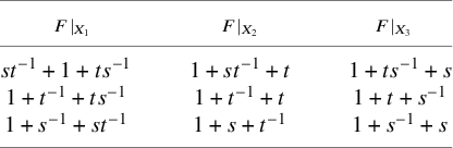


For this case, we added a few extra pieces of data in the end, to show how large the numbers become. Notice that the last example has a denominator of $2^{24}$
. It looks very complicated, but in this case,
$2^{24}$
. It looks very complicated, but in this case, $k = 0$
, so it follows from Proposition 2.5!
$k = 0$
, so it follows from Proposition 2.5!


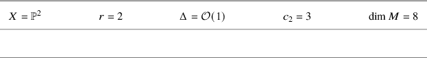


In this case we have added some extra computations for your interest.


Note the symmetry between this case and the previous, which is obtained by interchanging F and Z.


In this case, Conjecture 1.4 is again automatic for dimension reasons.

We listed only one table for $X = \mathbb {F}_2$
because the conjecture follows from the
$X = \mathbb {F}_2$
because the conjecture follows from the $X = \mathbb {F}_0$
case. We kept this table so that the reader can note that this table does not exactly match the table for the corresponding
$X = \mathbb {F}_0$
case. We kept this table so that the reader can note that this table does not exactly match the table for the corresponding $X = \mathbb {F}_0$
case, which is
$X = \mathbb {F}_0$
case, which is $r = 2$
,
$r = 2$
, $\Delta = F$
and
$\Delta = F$
and $c_2 = 1$
(see above). The reason is that the deformation does not preserve Z.
$c_2 = 1$
(see above). The reason is that the deformation does not preserve Z.


Acknowledgments
The author would like to thank his supervisor Martijn Kool for many useful suggestions and learning from him many of the techniques employed in this paper. He is also grateful to Rahul Pandharipande for raising the problem addressed in this paper in his Hangzhou lecture as well as provding some references. Furthemore, he would like to thank Sergej Monavari, Woonam Lim, Longting Wu and Carel Faber for insightful comments. Finally, he appreciates the thorough reading of the draft version of this paper by the referee. The author is supported by NWO grant VI.Vidi.192.012.
Conflict of Interest
The authors have no conflict of interest to declare.
Financial support
The author is supported by NWO grant VI.Vidi.192.012.


 Open access