


1 Introduction and main results
1.1 Introduction
Given an ergodic measure preserving system $(X, \mu ,T)$
and functions
$(X, \mu ,T)$
and functions $f,g\in L^\infty (\mu )$
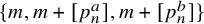
, it was shown in [Reference Frantzikinakis6] that for distinct
$f,g\in L^\infty (\mu )$
, it was shown in [Reference Frantzikinakis6] that for distinct $a,b\in {\mathbb R}_+\setminus {\mathbb Z}$
, we have
$a,b\in {\mathbb R}_+\setminus {\mathbb Z}$
, we have
 $$ \begin{align} \lim_{N\to\infty} \frac{1}{N}\sum_{n=1}^N \, T^{[n^a]}f\cdot T^{[n^b]}g=\int f\, d\mu \cdot \int g\, d\mu\\[-16pt]\nonumber \end{align} $$
in $L^2(\mu )$
.Footnote
1
An immediate consequence of this limit formula is that for every (not necessarily ergodic) measure preserving system and measurable set A, we have
$L^2(\mu )$
.Footnote
1
An immediate consequence of this limit formula is that for every (not necessarily ergodic) measure preserving system and measurable set A, we have
 $$ \begin{align} \lim_{N\to\infty} \frac{1}{N}\sum_{n=1}^N \, \mu(A\cap T^{-[n^a]}A\cap T^{-[n^b]}A)\geq \mu(A)^3.\\[-16pt]\nonumber \end{align} $$
Examples of periodic systems show that equations (1) and (2) fail if either a or b is an integer greater than $1$
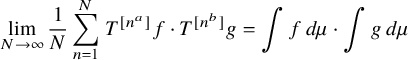
. Using the Furstenberg correspondence principle [Reference Furstenberg10, Reference Furstenberg11], it is easy to deduce from equation (2) that every set of integers with positive upper density contains patterns of the form
$1$
. Using the Furstenberg correspondence principle [Reference Furstenberg10, Reference Furstenberg11], it is easy to deduce from equation (2) that every set of integers with positive upper density contains patterns of the form
 $$ \begin{align*}\{m,m+[n^a],m+[n^b]\}\\[-16pt] \end{align*} $$
for some $m,n\in {\mathbb N}$
.
$m,n\in {\mathbb N}$
.
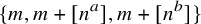
The main goal of this article is to establish similar convergence and multiple recurrence results, and deduce related combinatorial consequences, when in the previous statements we replace the variable n with the nth prime number $p_n$
. For instance, we show in Theorem 1.1 that if
$p_n$
. For instance, we show in Theorem 1.1 that if $a,b\in {\mathbb R}_+$
are distinct nonintegers, then
$a,b\in {\mathbb R}_+$
are distinct nonintegers, then
 $$ \begin{align} \lim_{N\to\infty} \frac{1}{N}\sum_{n=1}^N \, T^{[p_n^a]}f\cdot T^{[p_n^b]}g=\int f\, d\mu \cdot \int g\, d\mu\\[-16pt]\nonumber \end{align} $$
in $L^2(\mu )$
. We also prove more general statements of this sort involving two or more linearly independent polynomials with fractional exponents evaluated at primes (related results for fractional powers of integers were previously established in [Reference Bergelson, Moreira and Richter4, Reference Frantzikinakis6, Reference Richter26]).
$L^2(\mu )$
. We also prove more general statements of this sort involving two or more linearly independent polynomials with fractional exponents evaluated at primes (related results for fractional powers of integers were previously established in [Reference Bergelson, Moreira and Richter4, Reference Frantzikinakis6, Reference Richter26]).
If $a,b\in {\mathbb N}$
are natural numbers, then equation (3) fails because of obvious congruence obstructions. On the other hand, using the method in [Reference Frantzikinakis, Host and Kra9], it can be shown that if
$a,b\in {\mathbb N}$
are natural numbers, then equation (3) fails because of obvious congruence obstructions. On the other hand, using the method in [Reference Frantzikinakis, Host and Kra9], it can be shown that if $a,b\in {\mathbb N}$
are distinct, then equation (3) does hold under the additional assumption that the system is totally ergodic; see also [Reference Karageorgos and Koutsogiannis19, Reference Koutsogiannis20] for related work regarding polynomials in
$a,b\in {\mathbb N}$
are distinct, then equation (3) does hold under the additional assumption that the system is totally ergodic; see also [Reference Karageorgos and Koutsogiannis19, Reference Koutsogiannis20] for related work regarding polynomials in ${\mathbb R}[t]$
evaluated at primes. The main idea in the proof of these results is to show that the difference of a modification of the averages in equation (3) and the averages equation (1) converges to
${\mathbb R}[t]$
evaluated at primes. The main idea in the proof of these results is to show that the difference of a modification of the averages in equation (3) and the averages equation (1) converges to $0$
in
$0$
in $L^2(\mu )$
. This comparison method works well when
$L^2(\mu )$
. This comparison method works well when $a,b$
are positive integers since, in this case, one can bound this difference by the Gowers uniformity norm of the modified von Mangoldt function
$a,b$
are positive integers since, in this case, one can bound this difference by the Gowers uniformity norm of the modified von Mangoldt function $\tilde {\Lambda }_N$
(see [Reference Frantzikinakis, Host and Kra9, Lemma 3.5] for the precise statement), which is known by [Reference Green and Tao14] to converge to
$\tilde {\Lambda }_N$
(see [Reference Frantzikinakis, Host and Kra9, Lemma 3.5] for the precise statement), which is known by [Reference Green and Tao14] to converge to $0$
as
$0$
as $N\to \infty $
. Unfortunately, if
$N\to \infty $
. Unfortunately, if $a,b$
are not integers, this comparison step breaks down, since it requires a uniformity property for
$a,b$
are not integers, this comparison step breaks down, since it requires a uniformity property for $\tilde {\Lambda }_N$
in which some of the averaging parameters lie in very short intervals, a property that is currently not known. An alternative approach for establishing equation (3) is given by the argument used in [Reference Frantzikinakis6] to prove equation (1). It uses the theory of characteristic factors that originates from [Reference Host and Kra16] and eventually reduces the problem to an equidistribution result on nilmanifolds. This method is also blocked since we are unable to establish the needed equidistribution properties on general nilmanifolds.Footnote
2
$\tilde {\Lambda }_N$
in which some of the averaging parameters lie in very short intervals, a property that is currently not known. An alternative approach for establishing equation (3) is given by the argument used in [Reference Frantzikinakis6] to prove equation (1). It uses the theory of characteristic factors that originates from [Reference Host and Kra16] and eventually reduces the problem to an equidistribution result on nilmanifolds. This method is also blocked since we are unable to establish the needed equidistribution properties on general nilmanifolds.Footnote
2
Our approach is quite different and is based on a recent result of the author from [Reference Frantzikinakis8] (see Theorem 2.1 below); it implies that in order to verify equation (3), it suffices to obtain suitable seminorm estimates and equidistribution results on the circle (versus the general nilmanifold that the method of characteristic factors requires). The needed equidistribution property follows from [Reference Bergelson, Kolesnik, Madritsch, Son and Tichy2] (see Theorem 2.2 below), and the bulk of this article is devoted to the rather tricky proof of the seminorm estimates (see Theorem 1.4 below).
1.2 Main results
To facilitate discussion, we use the following definition from [Reference Frantzikinakis8].
Definition. We say that the collection of sequences $b_1,\ldots , b_\ell \colon {\mathbb N}\to {\mathbb Z}$
is jointly ergodic if, for every ergodic system
$b_1,\ldots , b_\ell \colon {\mathbb N}\to {\mathbb Z}$
is jointly ergodic if, for every ergodic system $(X,\mu ,T)$
and functions
$(X,\mu ,T)$
and functions $f_1,\ldots , f_\ell \in L^\infty (\mu )$
, we have
$f_1,\ldots , f_\ell \in L^\infty (\mu )$
, we have
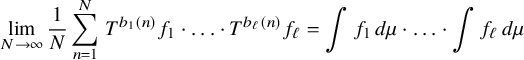 $$ \begin{align*} \lim_{N\to\infty} \frac{1}{N}\sum_{n=1}^N \, T^{b_1(n)}f_1 \cdot\ldots \cdot T^{b_\ell(n)}f_\ell= \int f_1\, d\mu\cdot \ldots \cdot \int f_\ell\, d\mu \end{align*} $$
in $L^2(\mu )$
.
$L^2(\mu )$
.
For instance, the identities in equations (1) and (3) are equivalent to the joint ergodicity of the pairs of sequences $\{[n^a], [n^b]\}$
and
$\{[n^a], [n^b]\}$
and $\{[p_n^a], [p_n^b]\}$
when
$\{[p_n^a], [p_n^b]\}$
when $a,b\in {\mathbb R}_+$
are distinct nonintegers.
$a,b\in {\mathbb R}_+$
are distinct nonintegers.
We will establish joint ergodicity properties involving the class of fractional polynomials that we define next.
Definition. A polynomial with real exponents is a function $a\colon {\mathbb R}_+\to {\mathbb R}$
of the form
$a\colon {\mathbb R}_+\to {\mathbb R}$
of the form $a(t)=\sum _{j=1}^r \alpha _jt^{d_j}$
, where
$a(t)=\sum _{j=1}^r \alpha _jt^{d_j}$
, where $\alpha _j\in {\mathbb R}$
and
$\alpha _j\in {\mathbb R}$
and $d_j\in {\mathbb R}_+$
,
$d_j\in {\mathbb R}_+$
, $j=1,\ldots , r$
. If
$j=1,\ldots , r$
. If $d_1,\ldots , d_r\in {\mathbb R}_+\setminus {\mathbb Z}$
, we call it a fractional polynomial.
$d_1,\ldots , d_r\in {\mathbb R}_+\setminus {\mathbb Z}$
, we call it a fractional polynomial.
The following is the main result of this article:
Theorem 1.1. Let $a_1,\ldots , a_\ell $
be linearly independentFootnote
3
fractional polynomials. Then the collection of sequences
$a_1,\ldots , a_\ell $
be linearly independentFootnote
3
fractional polynomials. Then the collection of sequences $[a_1(p_n)],\ldots , [a_\ell (p_n)]$
is jointly ergodic.
$[a_1(p_n)],\ldots , [a_\ell (p_n)]$
is jointly ergodic.
In particular, this applies to the collection of sequences $[n^{c_1}],\ldots , [n^{c_\ell }]$
, where
$[n^{c_1}],\ldots , [n^{c_\ell }]$
, where $c_1,\ldots , c_\ell \in {\mathbb R}_+\setminus {\mathbb Z}$
are distinct. We remark also that the linear independence assumption is necessary for joint ergodicity. Indeed, suppose that
$c_1,\ldots , c_\ell \in {\mathbb R}_+\setminus {\mathbb Z}$
are distinct. We remark also that the linear independence assumption is necessary for joint ergodicity. Indeed, suppose that $a_1,\ldots ,a_\ell $
is a collection of linearly depended sequences. Then
$a_1,\ldots ,a_\ell $
is a collection of linearly depended sequences. Then $c_1a_1+\cdots +c_\ell a_\ell =0$
for some
$c_1a_1+\cdots +c_\ell a_\ell =0$
for some $c_1,\ldots , c_\ell \in {\mathbb R}$
not all of them
$c_1,\ldots , c_\ell \in {\mathbb R}$
not all of them $0$
. After multiplying by an appropriate constant, we can assume that at least one of the
$0$
. After multiplying by an appropriate constant, we can assume that at least one of the $c_1,\ldots , c_\ell $
is not an integer and
$c_1,\ldots , c_\ell $
is not an integer and $\max _{i=1,\ldots , \ell }|c_i|\leq 1/(10\ell )$
. Then
$\max _{i=1,\ldots , \ell }|c_i|\leq 1/(10\ell )$
. Then $c_1[a_1(n)]+\cdots +c_\ell [a_\ell (n)]\in [-1/10,1/10]$
for all
$c_1[a_1(n)]+\cdots +c_\ell [a_\ell (n)]\in [-1/10,1/10]$
for all $n\in {\mathbb N}$
, and this easily implies that the collection
$n\in {\mathbb N}$
, and this easily implies that the collection $[a_1(n)],\ldots , [a_\ell (n)]$
is not good for equidistribution (see definition in Section 2) and hence not jointly ergodic.
$[a_1(n)],\ldots , [a_\ell (n)]$
is not good for equidistribution (see definition in Section 2) and hence not jointly ergodic.
Using standard methods, we immediately deduce from Theorem 1.1 the following multiple recurrence result:
Corollary 1.2. Let $a_1,\ldots , a_\ell $
be linearly independent fractional polynomials. Then for every system
$a_1,\ldots , a_\ell $
be linearly independent fractional polynomials. Then for every system $(X,\mu ,T)$
and measurable set A, we have
$(X,\mu ,T)$
and measurable set A, we have
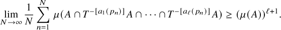 $$ \begin{align*} \lim_{N\to\infty} \frac{1}{N}\sum_{n=1}^N \, \mu(A\cap T^{-[a_1(p_n)]}A\cap\cdots\cap T^{-[a_{\ell}(p_n)]}A)\geq (\mu(A))^{\ell+1}. \end{align*} $$
Using the Furstenberg correspondence principle [Reference Furstenberg10, Reference Furstenberg11], we deduce the following combinatorial consequence:
Corollary 1.3. Let $a_1,\ldots , a_\ell $
be linearly independent fractional polynomials. Then for every subset
$a_1,\ldots , a_\ell $
be linearly independent fractional polynomials. Then for every subset $\Lambda $
of
$\Lambda $
of ${\mathbb N}$
, we haveFootnote
4
${\mathbb N}$
, we haveFootnote
4
 $$ \begin{align*} \liminf_{N\to\infty} \frac{1}{N}\sum_{n=1}^N \, \bar{d}(\Lambda\cap (\Lambda -[a_1(p_n)])\cap \cdots \cap (\Lambda -[a_\ell(p_n)]))\geq (\bar{d}(\Lambda))^{\ell+1}.\\[-15pt] \end{align*} $$
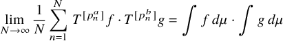
Hence, every set of integers with positive upper density contains patterns of the form $\{m,m+[a_1(p_n)], \ldots , m+[a_\ell (p_n)] \}$
for some
$\{m,m+[a_1(p_n)], \ldots , m+[a_\ell (p_n)] \}$
for some $m,n\in {\mathbb N}$
.
$m,n\in {\mathbb N}$
.
An essential tool in the proof of our main result is the following statement that is of independent interest since it covers a larger class of collections of fractional polynomials (not necessarily linearly independent) evaluated at primes. See Section 2 for the definition of the seminorms $\lvert \!|\!| \cdot |\!|\!\rvert _s$
.
$\lvert \!|\!| \cdot |\!|\!\rvert _s$
.
Theorem 1.4. Suppose that the fractional polynomials $a_1,\ldots , a_\ell $
and their pairwise differences are nonzero. Then there exists
$a_1,\ldots , a_\ell $
and their pairwise differences are nonzero. Then there exists $s\in {\mathbb N}$
such that for every ergodic system
$s\in {\mathbb N}$
such that for every ergodic system $(X,\mu ,T)$
and functions
$(X,\mu ,T)$
and functions $f_1,\ldots , f_\ell \in L^\infty (\mu )$
with
$f_1,\ldots , f_\ell \in L^\infty (\mu )$
with $\lvert \!|\!| f_i|\!|\!\rvert _{s}=0$
for some
$\lvert \!|\!| f_i|\!|\!\rvert _{s}=0$
for some $i\in \{1,\ldots , \ell \}$
, we have
$i\in \{1,\ldots , \ell \}$
, we have
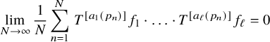 $$ \begin{align} \lim_{N\to\infty} \frac{1}{N}\sum_{n=1}^N\, T^{[a_1(p_n)]}f_1\cdot \ldots \cdot T^{[a_\ell(p_n)]}f_\ell=0\\[-15pt]\nonumber \end{align} $$
in $L^2(\mu )$
.
$L^2(\mu )$
.
Remark. It seems likely that with some additional effort the techniques of this article can cover the more general case of Hardy field functions $a_1,\ldots , a_\ell $
such that the functions and their differences belong to the set
$a_1,\ldots , a_\ell $
such that the functions and their differences belong to the set $\{a\colon {\mathbb R}_+\to {\mathbb R}\colon t^{k+\varepsilon }\prec a(t)\prec t^{k+1-\varepsilon } \text { for some } k\in {\mathbb Z}_+ \text { and } \varepsilon>0\}$
. Using the equidistribution result in [Reference Bergelson, Kolesnik and Son3] and the argument in Section 2, this would immediately give a corresponding strengthening of Theorem 1.1. We opted not to deal with these more general statements because the added technical complexity would obscure the main ideas of the proof of Theorem 1.4.
$\{a\colon {\mathbb R}_+\to {\mathbb R}\colon t^{k+\varepsilon }\prec a(t)\prec t^{k+1-\varepsilon } \text { for some } k\in {\mathbb Z}_+ \text { and } \varepsilon>0\}$
. Using the equidistribution result in [Reference Bergelson, Kolesnik and Son3] and the argument in Section 2, this would immediately give a corresponding strengthening of Theorem 1.1. We opted not to deal with these more general statements because the added technical complexity would obscure the main ideas of the proof of Theorem 1.4.
The proof of Theorem 1.4 crucially uses the fact that the iterates $a_1,\ldots , a_\ell $
have ‘fractional power growth’, and our argument fails for iterates with ‘integer power growth’. Similar results that cover the case of polynomials with integer or real coefficients were obtained in [Reference Frantzikinakis, Host and Kra9, Reference Wooley and Ziegler29] and [Reference Karageorgos and Koutsogiannis19], respectively, and depend on deep properties of the von Mangoldt function from [Reference Green and Tao13] and [Reference Green and Tao14], but these results and their proofs do not appear to be useful for our purposes. Instead, we rely on some softer number theory input that follows from standard sieve theory techniques (see Section 3.2) and an argument that is fine-tuned for the case of fractional polynomials (but fails for polynomials with integer exponents). This argument eventually enables us to bound the averages in equation (4) with averages involving iterates given by multivariate polynomials with real coefficients evaluated at the integers, a case that was essentially handled in [Reference Leibman23].
$a_1,\ldots , a_\ell $
have ‘fractional power growth’, and our argument fails for iterates with ‘integer power growth’. Similar results that cover the case of polynomials with integer or real coefficients were obtained in [Reference Frantzikinakis, Host and Kra9, Reference Wooley and Ziegler29] and [Reference Karageorgos and Koutsogiannis19], respectively, and depend on deep properties of the von Mangoldt function from [Reference Green and Tao13] and [Reference Green and Tao14], but these results and their proofs do not appear to be useful for our purposes. Instead, we rely on some softer number theory input that follows from standard sieve theory techniques (see Section 3.2) and an argument that is fine-tuned for the case of fractional polynomials (but fails for polynomials with integer exponents). This argument eventually enables us to bound the averages in equation (4) with averages involving iterates given by multivariate polynomials with real coefficients evaluated at the integers, a case that was essentially handled in [Reference Leibman23].
1.3 Limitations of our techniques and open problems
We expect that the following generalisation of Theorem 1.1 holds:
Problem. Let $a_1,\ldots ,a_\ell $
be functions from a Hardy field with polynomial growth such that every nontrivial linear combination b of them satisfies
$a_1,\ldots ,a_\ell $
be functions from a Hardy field with polynomial growth such that every nontrivial linear combination b of them satisfies $ |b(t)-p(t)|/\log {t}\to \infty $
for all
$ |b(t)-p(t)|/\log {t}\to \infty $
for all $p\in {\mathbb Z}[t]$
. Then the collection of sequences
$p\in {\mathbb Z}[t]$
. Then the collection of sequences $[a_1(p_n)],\ldots , [a_\ell (p_n)]$
is jointly ergodic.
$[a_1(p_n)],\ldots , [a_\ell (p_n)]$
is jointly ergodic.
By Theorem 2.1, it suffices to show that the collection $[a_1(p_n)],\ldots , [a_\ell (p_n)]$
is good for equidistribution and seminorm estimates. Although the needed equidistribution property has been proved in [Reference Bergelson, Kolesnik and Son3, Theorem 3.1], the seminorm estimates that extend Theorem 1.4 seem hard to establish. Our argument breaks down when some of the functions, or their differences, are close to integral powers of t: for example, when they are
$[a_1(p_n)],\ldots , [a_\ell (p_n)]$
is good for equidistribution and seminorm estimates. Although the needed equidistribution property has been proved in [Reference Bergelson, Kolesnik and Son3, Theorem 3.1], the seminorm estimates that extend Theorem 1.4 seem hard to establish. Our argument breaks down when some of the functions, or their differences, are close to integral powers of t: for example, when they are $t^k\log {t}$
or
$t^k\log {t}$
or $t^k/\log \log {t}$
for some
$t^k/\log \log {t}$
for some $k\in {\mathbb N}$
. In both cases, the vdC-operation (see Section 5.2) leads to sequences of sublinear growth for which we can no longer establish Lemma 4.1, in the first case because the estimate equation (20) fails and in the second case because in equation (22), the length of the interval in the average is too short for Corollary 3.4 to be applicable.
$k\in {\mathbb N}$
. In both cases, the vdC-operation (see Section 5.2) leads to sequences of sublinear growth for which we can no longer establish Lemma 4.1, in the first case because the estimate equation (20) fails and in the second case because in equation (22), the length of the interval in the average is too short for Corollary 3.4 to be applicable.
Finally, we remark that although the reduction offered by Theorem 2.1 is very helpful when dealing with averages with independent iterates, as is the case in equation (3), it does not offer any help when the iterates are linearly dependent, which is the case for the averages
 $$ \begin{align} \frac{1}{N}\sum_{n=1}^N \, T^{[p_n^{a}]}f\cdot T^{2[p_n^a]}g, \end{align} $$
where $a\in {\mathbb R}_+$
is not an integer. We do expect the
$a\in {\mathbb R}_+$
is not an integer. We do expect the $L^2(\mu )$
-limit of the averages in equation (5) to be equal to the
$L^2(\mu )$
-limit of the averages in equation (5) to be equal to the $L^2(\mu )$
-limit of the averages
$L^2(\mu )$
-limit of the averages $ \frac {1}{N}\sum _{n=1}^N \,T^{n}f\cdot T^{2n}g$
, but this remains a challenging open problemFootnote
5
; see Problem 27 in [Reference Frantzikinakis7].
$ \frac {1}{N}\sum _{n=1}^N \,T^{n}f\cdot T^{2n}g$
, but this remains a challenging open problemFootnote
5
; see Problem 27 in [Reference Frantzikinakis7].
1.4 Notation
With ${\mathbb N}$
, we denote the set of positive integers, and with
${\mathbb N}$
, we denote the set of positive integers, and with ${\mathbb Z}_+$
, the set of nonnegative integers. With
${\mathbb Z}_+$
, the set of nonnegative integers. With ${\mathbb P}$
, we denote the set of prime numbers. With
${\mathbb P}$
, we denote the set of prime numbers. With ${\mathbb R}_+$
, we denote the set of nonnegative real numbers. For
${\mathbb R}_+$
, we denote the set of nonnegative real numbers. For $t\in {\mathbb R}$
, we let
$t\in {\mathbb R}$
, we let $e(t):=e^{2\pi i t}$
. If
$e(t):=e^{2\pi i t}$
. If $x\in {\mathbb R}_+$
, when there is no danger for confusion, with
$x\in {\mathbb R}_+$
, when there is no danger for confusion, with $[x]$
, we denote both the integer part of x and the set
$[x]$
, we denote both the integer part of x and the set $\{1,\ldots , [x]\}$
. We denote with
$\{1,\ldots , [x]\}$
. We denote with $\Re (z)$
the real part of the complex number z.
$\Re (z)$
the real part of the complex number z.
Let $a\colon {\mathbb N}\to {\mathbb C}$
be a bounded sequence. If A is a nonempty finite subset of
$a\colon {\mathbb N}\to {\mathbb C}$
be a bounded sequence. If A is a nonempty finite subset of ${\mathbb N}$
, we let
${\mathbb N}$
, we let
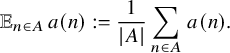 $$ \begin{align*}{\mathbb E}_{n\in A}\,a(n):=\frac{1}{|A|}\sum_{n\in A}\, a(n). \end{align*} $$
If $a,b\colon {\mathbb R}_+\to {\mathbb R}$
are functions, we write
$a,b\colon {\mathbb R}_+\to {\mathbb R}$
are functions, we write
-
○ $a(t)\prec b(t)$
if
$\lim _{t\to +\infty } a(t)/b(t)=0$
;
$a(t)\prec b(t)$
if
$\lim _{t\to +\infty } a(t)/b(t)=0$
; -
○
$a(t)\sim b(t)$
if
$\lim _{t\to +\infty } a(t)/b(t)$
exists and is nonzero; -
○
$A_{c_1,\ldots , c_\ell }(t)\ll _{c_1,\ldots , c_\ell } B_{c_1,\ldots , c_\ell }(t)$
if there exist
$t_0=t_0(c_1,\ldots , c_\ell )\in {\mathbb R}_+$
and
$C=C(c_1,\ldots , c_\ell )>0$
such that
$|A_{c_1,\ldots , c_\ell }(t)|\leq C |B_{c_1,\ldots , c_\ell }(t)|$
for all
$t\geq t_0$
.


We use the same notation for sequences $a,b\colon {\mathbb N}\to {\mathbb R}$
.
$a,b\colon {\mathbb N}\to {\mathbb R}$
.
Throughout, we let $L_N:=[e^{\sqrt {\log {N}}}]$
,
$L_N:=[e^{\sqrt {\log {N}}}]$
, $N\in {\mathbb N}$
.
$N\in {\mathbb N}$
.
We say that a sequence $(c_{N,{\underline {h}}}(n))$
, where
$(c_{N,{\underline {h}}}(n))$
, where ${\underline {h}}\in [L_N]^k$
,
${\underline {h}}\in [L_N]^k$
, $n\in [N]$
,
$n\in [N]$
, $N\in {\mathbb N}$
, is bounded if there exists C>0 such that
$N\in {\mathbb N}$
, is bounded if there exists C>0 such that $|c_{N,{\underline {h}}}(n)|\leq C$
for all
$|c_{N,{\underline {h}}}(n)|\leq C$
for all ${\underline {h}}\in [L_N]^k$
,
${\underline {h}}\in [L_N]^k$
, $n\in [N]$
,
$n\in [N]$
, $N\in {\mathbb N}$
.
$N\in {\mathbb N}$
.
2 Proof strategy
Our argument depends upon a convenient criterion for joint ergodicity that was established recently in [Reference Frantzikinakis8] (and was motivated by work in [Reference Peluse24, Reference Peluse and Prendiville25]). To state it, we need to review the definition of the ergodic seminorms from [Reference Host and Kra16].
Definition. For a given ergodic system $(X,\mu ,T)$
and function
$(X,\mu ,T)$
and function $f\in L^\infty (\mu )$
, we define
$f\in L^\infty (\mu )$
, we define $\lvert \!|\!| \cdot |\!|\!\rvert _s$
inductively as follows:
$\lvert \!|\!| \cdot |\!|\!\rvert _s$
inductively as follows:
 $$ \begin{align*} \lvert\!|\!| f|\!|\!\rvert_{1}\mathrel{\mathop:} &=\Big| \int f \ d\mu\Big|\ ;\\ \lvert\!|\!| f|\!|\!\rvert_{s+1}^{2^{s+1}} \mathrel{\mathop:}=\lim_{N\to\infty}\frac{1}{N} &\sum_{n=1}^{N} \lvert\!|\!| \overline{f}\cdot T^nf|\!|\!\rvert_{s}^{2^{s}}, \quad s\in {\mathbb N}. \end{align*} $$
It was shown in [Reference Host and Kra16], via successive uses of the mean ergodic theorem, that for every $s\in {\mathbb N}$
, the above limit exists, and
$s\in {\mathbb N}$
, the above limit exists, and $\lvert \!|\!| \cdot |\!|\!\rvert _s$
defines an increasing sequence of seminorms on
$\lvert \!|\!| \cdot |\!|\!\rvert _s$
defines an increasing sequence of seminorms on $L^\infty (\mu )$
.
$L^\infty (\mu )$
.
Definition. We say that the collection of sequences $b_1,\ldots , b_\ell \colon {\mathbb N}\to {\mathbb Z}$
is:
$b_1,\ldots , b_\ell \colon {\mathbb N}\to {\mathbb Z}$
is:
-
1. Good for seminorm estimates, if for every ergodic system
$(X,\mu ,T)$
, there exists
$s\in {\mathbb N}$
such that if
$f_1,\ldots , f_\ell \in L^\infty (\mu )$
and
$\lvert \!|\!| f_m|\!|\!\rvert _{s}=0$
for some
$m\in \{1,\ldots , \ell \}$
, then (6)in
$$ \begin{align} \lim_{N\to\infty} {\mathbb E}_{n\in [N]}\, T^{b_1(n)}f_1\cdot\ldots \cdot T^{b_m(n)}f_m= 0 \end{align} $$
$L^2(\mu )$
.Footnote
6
-
2. Good for equidistribution, if for all
$t_1,\ldots , t_\ell \in [0,1)$
, not all of them
$0$
, we have
$$ \begin{align*} \lim_{N\to\infty} {\mathbb E}_{n\in[N]}\, e(b_1(n)t_1+\cdots+ b_\ell(n)t_\ell) =0. \end{align*} $$


We remark that any collection of nonconstant integer polynomial sequences with pairwise nonconstant differences is known to be good for seminorm estimates [Reference Leibman23], and examples of periodic systems show that no such collection is good for equidistribution (unless $\ell =1$
and
$\ell =1$
and $b_1(t)=\pm t+k$
). On the other hand, a collection of linearly independent fractional polynomials is known to be good both for seminorm estimates [Reference Frantzikinakis6, Theorem 2.9] and equidistribution (follows from [Reference Kuipers and Niederreiter22, Theorem 3.4] and [Reference Frantzikinakis8, Lemma 6.2]).
$b_1(t)=\pm t+k$
). On the other hand, a collection of linearly independent fractional polynomials is known to be good both for seminorm estimates [Reference Frantzikinakis6, Theorem 2.9] and equidistribution (follows from [Reference Kuipers and Niederreiter22, Theorem 3.4] and [Reference Frantzikinakis8, Lemma 6.2]).
A crucial ingredient used in the proof of our main result is the following result that gives convenient necessary and sufficient conditions for joint ergodicity of a collection of sequences (see also [Reference Best and Moragues5] for an extension of this result for sequences $b_1,\ldots , b_\ell \colon {\mathbb N}^k\to {\mathbb Z}$
).
$b_1,\ldots , b_\ell \colon {\mathbb N}^k\to {\mathbb Z}$
).
Theorem 2.1 ([Reference Frantzikinakis8])
The sequences $b_1,\ldots , b_\ell \colon {\mathbb N}\to {\mathbb Z}$
are jointly ergodic if and only if they are good for equidistribution and seminorm estimates.
$b_1,\ldots , b_\ell \colon {\mathbb N}\to {\mathbb Z}$
are jointly ergodic if and only if they are good for equidistribution and seminorm estimates.
Remark. The proof of this result uses ‘soft’ tools from ergodic theory and avoids deeper tools like the Host-Kra theory of characteristic factors (see [Reference Host and Kra17, Chapter 21] for a detailed description) and equidistribution results on nilmanifolds.
In view of this result, in order to establish Theorem 1.1, it suffices to show that a collection of linearly independent fractional polynomials evaluated at primes is good for seminorm estimates and equidistribution. The good equidistribution property is a consequence of the following result [Reference Bergelson, Kolesnik, Madritsch, Son and Tichy2, Theorem 2.1]:
Theorem 2.2 ([Reference Bergelson, Kolesnik, Madritsch, Son and Tichy2])
If $a(t)$
is a nonzero fractional polynomial, then the sequence
$a(t)$
is a nonzero fractional polynomial, then the sequence $(a(p_n))$
is equidistributed
$(a(p_n))$
is equidistributed $\! \! \pmod {1}$
.
$\! \! \pmod {1}$
.
Using the previous result and [Reference Frantzikinakis8, Lemma 6.2], we immediately deduce the following:
Corollary 2.3. If $a_1,\ldots , a_\ell $
are linearly independent fractional polynomials, then the collection of sequences
$a_1,\ldots , a_\ell $
are linearly independent fractional polynomials, then the collection of sequences $[a_1(p_n)], \ldots , [a_\ell (p_n)]$
is good for equidistribution.
$[a_1(p_n)], \ldots , [a_\ell (p_n)]$
is good for equidistribution.
We let $\Lambda '\colon {\mathbb N}\to {\mathbb R}_+$
be the following slight modification of the von Mangoldt function:
$\Lambda '\colon {\mathbb N}\to {\mathbb R}_+$
be the following slight modification of the von Mangoldt function: $\Lambda '(n):=\log (n)$
if n is a prime number and
$\Lambda '(n):=\log (n)$
if n is a prime number and $0$
otherwise. To establish that the collection
$0$
otherwise. To establish that the collection $[a_1(p_n)], \ldots , [a_\ell (p_n)]$
is good for seminorm estimates, it suffices to prove the following result (the case
$[a_1(p_n)], \ldots , [a_\ell (p_n)]$
is good for seminorm estimates, it suffices to prove the following result (the case $w_N(n):=\Lambda '(n)$
,
$w_N(n):=\Lambda '(n)$
, $N,n\in {\mathbb N}$
, implies Theorem 1.4 in a standard way; see, for example, [Reference Frantzikinakis, Host and Kra9, Lemma 2.1]):
$N,n\in {\mathbb N}$
, implies Theorem 1.4 in a standard way; see, for example, [Reference Frantzikinakis, Host and Kra9, Lemma 2.1]):
Theorem 2.4. Suppose that the fractional polynomials $a_1,\ldots , a_\ell $
and their pairwise differences are nonzero. Then there exists
$a_1,\ldots , a_\ell $
and their pairwise differences are nonzero. Then there exists $s\in {\mathbb N}$
such that the following holds: If
$s\in {\mathbb N}$
such that the following holds: If $(X,\mu ,T)$
is an ergodic system and
$(X,\mu ,T)$
is an ergodic system and $f_1,\ldots , f_\ell \in L^\infty (\mu )$
are such that
$f_1,\ldots , f_\ell \in L^\infty (\mu )$
are such that $\lvert \!|\!| f_i|\!|\!\rvert _{s}=0$
for some
$\lvert \!|\!| f_i|\!|\!\rvert _{s}=0$
for some $i\in \{1,\ldots , \ell \}$
, then for every
$i\in \{1,\ldots , \ell \}$
, then for every $1$
-bounded sequence
$1$
-bounded sequence $(c_{N}(n))$
, we have
$(c_{N}(n))$
, we have
 $$ \begin{align} \lim_{N\to\infty} {\mathbb E}_{n\in [N]}\, w_N(n) \cdot T^{[a_1(n)]}f_1\cdot \ldots \cdot T^{[a_\ell(n)]}f_\ell=0 \end{align} $$
in $L^2(\mu )$
, where
$L^2(\mu )$
, where $w_N(n):=\Lambda '(n)\cdot c_N(n)$
,
$w_N(n):=\Lambda '(n)\cdot c_N(n)$
, $n\in [N]$
,
$n\in [N]$
, $N\in {\mathbb N}$
.
$N\in {\mathbb N}$
.
Remarks.
-
○ The sequence
$(c_N(n))$
is not essential in order to deduce Theorem 1.4. It is used because it helps us absorb error terms that often appear in our argument. -
○ Our proof shows that the place of the sequence
$(\Lambda '(n))$
can take any nonnegative sequence
$(b(n))$
that satisfies properties
$(i)$
and
$(ii)$
of Corollary 3.4 and the estimate
$b(n)\ll n^\varepsilon $
for every
$\varepsilon>0$
.


To prove Theorem 2.4, we use an induction argument, similar to the polynomial exhaustion technique (PET-induction) introduced in [Reference Bergelson1], which is based on variants of the van der Corput inequality stated immediately after Lemma 3.5. The fact that the weight sequence $(w_N(n))$
is unbounded forces us to apply Lemma 3.5 in the form given in equation (15) with
$(w_N(n))$
is unbounded forces us to apply Lemma 3.5 in the form given in equation (15) with $L_N\in {\mathbb N}$
that satisfy
$L_N\in {\mathbb N}$
that satisfy $L_N\succ (\log {N})^A$
for every
$L_N\succ (\log {N})^A$
for every $A>0$
. On the other hand, since we have to take care of some error terms that are of the order
$A>0$
. On the other hand, since we have to take care of some error terms that are of the order $L_N^B/N^a$
for arbitrary
$L_N^B/N^a$
for arbitrary $a, B>0$
, we are also forced to take
$a, B>0$
, we are also forced to take $L_N\prec N^a$
for every
$L_N\prec N^a$
for every $a>0$
in order for these errors to be negligible. These two estimates are satisfied for example when
$a>0$
in order for these errors to be negligible. These two estimates are satisfied for example when $L_N=[e^{\sqrt {\log {N}}}]$
,
$L_N=[e^{\sqrt {\log {N}}}]$
, $N\in {\mathbb N}$
, which is the value of
$N\in {\mathbb N}$
, which is the value of $L_N$
that we use henceforth.
$L_N$
that we use henceforth.
During the course of the PET-induction argument, we have to keep close track of the additional parameters $h_1,\ldots , h_k$
that arise after each application of Lemma 3.5 in the form given in equation (15). This is why we prove a more general variant of Theorem 2.4 that is stated in Theorem 3.1 and involves fractional polynomials with coefficients depending on finitely many parameters. It turns out that the most laborious part of its proof is the base case of the induction where all iterates have sublinear growth. This case is dealt with in three steps. First, in Lemma 4.1, we use a change of variables argument and the number theory input from Corollary 3.4 to reduce matters to the case where the weight sequence
$h_1,\ldots , h_k$
that arise after each application of Lemma 3.5 in the form given in equation (15). This is why we prove a more general variant of Theorem 2.4 that is stated in Theorem 3.1 and involves fractional polynomials with coefficients depending on finitely many parameters. It turns out that the most laborious part of its proof is the base case of the induction where all iterates have sublinear growth. This case is dealt with in three steps. First, in Lemma 4.1, we use a change of variables argument and the number theory input from Corollary 3.4 to reduce matters to the case where the weight sequence $(w_N(n))$
is bounded. Next, in Lemma 4.2, we use another change of variables argument and Lemma 3.5 to successively ‘eliminate’ the sequences
$(w_N(n))$
is bounded. Next, in Lemma 4.2, we use another change of variables argument and Lemma 3.5 to successively ‘eliminate’ the sequences $a_1, \ldots , a_\ell $
, and, after
$a_1, \ldots , a_\ell $
, and, after $\ell $
-iterations, we get an upper bound that involves iterates given by the integer parts of polynomials in several variables with real coefficients. Finally, in Lemma 4.3, we show that averages with such iterates obey good seminorm bounds. This last step is carried out by adapting an argument from [Reference Leibman23] to our setup; this is done by another PET-induction, which this time uses Lemma 3.5 in the form given in equation (16). In Sections 4.1 and 5.1, the reader will find examples that explain how these arguments work in some model cases that contain the essential ideas of the general arguments.
$\ell $
-iterations, we get an upper bound that involves iterates given by the integer parts of polynomials in several variables with real coefficients. Finally, in Lemma 4.3, we show that averages with such iterates obey good seminorm bounds. This last step is carried out by adapting an argument from [Reference Leibman23] to our setup; this is done by another PET-induction, which this time uses Lemma 3.5 in the form given in equation (16). In Sections 4.1 and 5.1, the reader will find examples that explain how these arguments work in some model cases that contain the essential ideas of the general arguments.
To conclude this section, we remark that to prove Theorem 1.1, it suffices to prove Theorem 2.4; the remaining sections are devoted to this task.
3 Seminorm estimates – some preparation
3.1 A more general statement
To prove Theorem 2.4, it will be convenient to establish a technically more complicated statement that is better suited for a PET-induction argument. We state it in this subsection.
Throughout, the sequence $L_N$
is chosen to satisfy
$L_N$
is chosen to satisfy $(\log {N})^A\prec L_N\prec N^a$
for all
$(\log {N})^A\prec L_N\prec N^a$
for all $A,a>0$
; so we can take, for example,
$A,a>0$
; so we can take, for example,
 $$ \begin{align*}L_N:=[e^{\sqrt{\log{N}}}], \quad N\in {\mathbb N}. \end{align*} $$
With ${\mathbb R}[t_1,\ldots , t_k]$
, we denote the set of polynomials with real coefficients in k-variables.
${\mathbb R}[t_1,\ldots , t_k]$
, we denote the set of polynomials with real coefficients in k-variables.
Definition. We say that $a\colon {\mathbb Z}^k\times {\mathbb R}_+\to {\mathbb R}$
is a polynomial with real exponents and k-parameters if it has the form
$a\colon {\mathbb Z}^k\times {\mathbb R}_+\to {\mathbb R}$
is a polynomial with real exponents and k-parameters if it has the form
 $$ \begin{align*} a({\underline{h}},t)=\sum_{j=0}^r p_j({\underline{h}})\, t^{d_j} \end{align*} $$
for some $r\in {\mathbb N}$
,
$r\in {\mathbb N}$
, $0=d_0<d_1<\cdots <d_r\in {\mathbb R}_+$
, and
$0=d_0<d_1<\cdots <d_r\in {\mathbb R}_+$
, and $p_0,\ldots , p_r\in {\mathbb R}[t_1,\ldots , t_k]$
. If
$p_0,\ldots , p_r\in {\mathbb R}[t_1,\ldots , t_k]$
. If $d_1,\ldots , d_r\in {\mathbb R}_+\setminus {\mathbb Z}$
, we call it a fractional polynomial with k-parameters. If
$d_1,\ldots , d_r\in {\mathbb R}_+\setminus {\mathbb Z}$
, we call it a fractional polynomial with k-parameters. If $p_j$
is nonzero for some
$p_j$
is nonzero for some $j\in \{1,\ldots , r\}$
, we say that
$j\in \{1,\ldots , r\}$
, we say that $a({\underline {h}},t)$
is nonconstant. We define the fractional degree of
$a({\underline {h}},t)$
is nonconstant. We define the fractional degree of $a({\underline {h}},t)$
to be the maximum exponent
$a({\underline {h}},t)$
to be the maximum exponent $d_j$
for which the polynomial
$d_j$
for which the polynomial $p_j$
is nonzero and denote it by
$p_j$
is nonzero and denote it by $\text {f-deg}(a)$
. We call the integer part of its fractional degree the (integral) degree of
$\text {f-deg}(a)$
. We call the integer part of its fractional degree the (integral) degree of $a({\underline {h}},t)$
and denote it by
$a({\underline {h}},t)$
and denote it by $\deg (a)$
. We also let
$\deg (a)$
. We also let $\deg (0):=-1$
.
$\deg (0):=-1$
.
For example, the fractional polynomial with $1$
-parameter
$1$
-parameter $h^2 t^{0.5}+(h^2\sqrt {2}+h)t^{0.1}$
has fractional degree
$h^2 t^{0.5}+(h^2\sqrt {2}+h)t^{0.1}$
has fractional degree $0.5$
and degree
$0.5$
and degree $0$
.
$0$
.
Definition. We say that a collection $a_1,\ldots , a_\ell $
of polynomials with real exponents and k-parameters is nice if
$a_1,\ldots , a_\ell $
of polynomials with real exponents and k-parameters is nice if
-
1.
$\text {f-deg}(a_i)\leq \text {f-deg}(a_1)$
for
$i=2,\ldots , \ell $
, and -
2. the functions
$a_1, \ldots a_\ell $
and the functions
$a_1-a_2, \ldots , a_1-a_\ell $
are nonconstant in the variable t (and as a consequence they have positive fractional degree).


Given a sequence $u\colon {\mathbb N}\to {\mathbb C}$
, we let
$u\colon {\mathbb N}\to {\mathbb C}$
, we let $(\Delta _hu)(n):=u(n+h)\cdot \overline {u(n)}$
,
$(\Delta _hu)(n):=u(n+h)\cdot \overline {u(n)}$
, $h,n\in {\mathbb N}$
, and if
$h,n\in {\mathbb N}$
, and if ${\underline {h}}=(h_1,\ldots , h_k)$
, we let
${\underline {h}}=(h_1,\ldots , h_k)$
, we let $(\Delta _{{\underline {h}}})(u(n)):=(\Delta _{h_k}\cdots \Delta _{h_1}) (u(n))$
,
$(\Delta _{{\underline {h}}})(u(n)):=(\Delta _{h_k}\cdots \Delta _{h_1}) (u(n))$
, $h_1,\ldots , h_k,n\in {\mathbb N}$
. For example,
$h_1,\ldots , h_k,n\in {\mathbb N}$
. For example, $(\Delta _{(h_1,h_2)})(u(n))= u(n+h_1+h_2)\cdot \overline {u}(n+h_1)\cdot \overline {u}(n+h_2)\cdot u(n)$
,
$(\Delta _{(h_1,h_2)})(u(n))= u(n+h_1+h_2)\cdot \overline {u}(n+h_1)\cdot \overline {u}(n+h_2)\cdot u(n)$
, $h_1,h_2,n\in {\mathbb N}$
.
$h_1,h_2,n\in {\mathbb N}$
.
Theorem 3.1. For $k\in {\mathbb Z}_+, \ell \in {\mathbb N}$
, let
$k\in {\mathbb Z}_+, \ell \in {\mathbb N}$
, let $a_1,\ldots , a_\ell \colon {\mathbb N}^k\times {\mathbb N}\to {\mathbb R}$
be a nice collection of fractional polynomials with k-parameters and
$a_1,\ldots , a_\ell \colon {\mathbb N}^k\times {\mathbb N}\to {\mathbb R}$
be a nice collection of fractional polynomials with k-parameters and $(c_{N,{\underline {h}}}(n))$
be a
$(c_{N,{\underline {h}}}(n))$
be a $1$
-bounded sequence. Then there exists
$1$
-bounded sequence. Then there exists $s\in {\mathbb N}$
such that the following holds: If
$s\in {\mathbb N}$
such that the following holds: If $(X,\mu ,T)$
is a system and
$(X,\mu ,T)$
is a system and $f_{N,{\underline {h}},1},\ldots , f_{N,{\underline {h}},\ell }\in L^\infty (\mu )$
,
$f_{N,{\underline {h}},1},\ldots , f_{N,{\underline {h}},\ell }\in L^\infty (\mu )$
, ${\underline {h}}\in [L_N]^k,N\in {\mathbb N}$
, are
${\underline {h}}\in [L_N]^k,N\in {\mathbb N}$
, are $1$
-bounded functions with
$1$
-bounded functions with $f_{N,{\underline {h}},1}=f_1$
,
$f_{N,{\underline {h}},1}=f_1$
, ${\underline {h}}\in {\mathbb N}^k,N\in {\mathbb N}$
and
${\underline {h}}\in {\mathbb N}^k,N\in {\mathbb N}$
and $\lvert \!|\!| f_1|\!|\!\rvert _s=0$
, then
$\lvert \!|\!| f_1|\!|\!\rvert _s=0$
, then
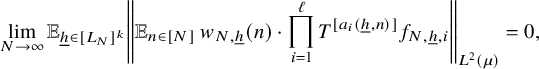 $$ \begin{align} \lim_{N\to\infty} {\mathbb E}_{\underline{h}\in [L_N]^k} \left\Vert {\mathbb E}_{n\in [N]}\, w_{N,\underline{h}}(n)\cdot \prod_{i=1}^\ell T^{[a_i(\underline{h},n)]}f_{N,{\underline{h}},i}\right\Vert_{L^2(\mu)}=0, \end{align} $$
where $w_{N,{\underline {h}}}(n):=(\Delta _{\underline {h}}\Lambda ')(n)\cdot c_{N,{\underline {h}}}(n)$
,
$w_{N,{\underline {h}}}(n):=(\Delta _{\underline {h}}\Lambda ')(n)\cdot c_{N,{\underline {h}}}(n)$
, $ {\underline {h}}\in [L_N]^k, n\in [N], N\in {\mathbb N}$
.
$ {\underline {h}}\in [L_N]^k, n\in [N], N\in {\mathbb N}$
.
Remark. Our argument also works if $\Delta _{\underline {h}}\Lambda '(n)$
is replaced by other expressions involving
$\Delta _{\underline {h}}\Lambda '(n)$
is replaced by other expressions involving $\Lambda '$
: for example, when
$\Lambda '$
: for example, when $k=0$
, one can use the expression
$k=0$
, one can use the expression $\prod _{i=1}^m\Lambda '(n+c_i)$
, where
$\prod _{i=1}^m\Lambda '(n+c_i)$
, where $c_1,\ldots , c_m$
are distinct integers.
$c_1,\ldots , c_m$
are distinct integers.
If in Theorem 3.1, we take $k=0$
, then we get Theorem 2.4 using an argument that we describe next.
$k=0$
, then we get Theorem 2.4 using an argument that we describe next.
Proof of Theorem 2.4 assuming Theorem 3.1
Let $a_1,\ldots , a_\ell $
and
$a_1,\ldots , a_\ell $
and $w_N(n)$
be as in Theorem 2.4. Since the assumptions of Theorem 2.4 are symmetric with respect to the sequences
$w_N(n)$
be as in Theorem 2.4. Since the assumptions of Theorem 2.4 are symmetric with respect to the sequences $a_1,\ldots , a_\ell $
, it suffices to show that there exists
$a_1,\ldots , a_\ell $
, it suffices to show that there exists $s\in {\mathbb N}$
such that if
$s\in {\mathbb N}$
such that if $\lvert \!|\!| f_1|\!|\!\rvert _s=0$
, then equation (7) holds.
$\lvert \!|\!| f_1|\!|\!\rvert _s=0$
, then equation (7) holds.
If $a_1$
has maximal fractional degree within the family
$a_1$
has maximal fractional degree within the family $a_1,\ldots a_\ell $
, then if we take
$a_1,\ldots a_\ell $
, then if we take $k=0$
and all functions to be independent of N in Theorem 3.1, we get that the conclusion of Theorem 2.4 holds. Otherwise, we can assume that
$k=0$
and all functions to be independent of N in Theorem 3.1, we get that the conclusion of Theorem 2.4 holds. Otherwise, we can assume that $a_{\ell }$
is the function with the highest fractional degree and, as a consequence,
$a_{\ell }$
is the function with the highest fractional degree and, as a consequence, $\text {f-deg}(a_1)<\text {f-deg}(a_\ell )$
. It suffices to show that
$\text {f-deg}(a_1)<\text {f-deg}(a_\ell )$
. It suffices to show that
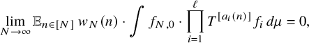 $$ \begin{align*} \lim_{N\to\infty} {\mathbb E}_{n\in [N]}\, w_{N}(n)\cdot \int f_{N,0} \cdot \prod_{i=1}^\ell T^{[a_i(n)]}f_{i} \, d\mu=0, \end{align*} $$
where
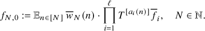 $$ \begin{align*} f_{N,0} := {\mathbb E}_{n\in [N]} \, \overline{w}_{N}(n)\cdot \prod_{i=1}^\ell T^{[a_i(n)]}\overline{f}_i, \quad N\in {\mathbb N}. \end{align*} $$
Note that since $f_1,\ldots , f_\ell $
and
$f_1,\ldots , f_\ell $
and $c_N$
are
$c_N$
are $1$
-bounded, we have
$1$
-bounded, we have
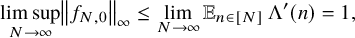 $$ \begin{align*} \limsup_{N\to\infty} \left\Vert f_{N,0}\right\Vert_\infty\leq \lim_{N\to\infty} {\mathbb E}_{n\in [N]} \, \Lambda'(n)=1, \end{align*} $$
(the last identity follows from the prime number theorem, but we only need the much simpler upper bound) hence, we can assume that $f_{N,0}$
is
$f_{N,0}$
is $1$
-bounded for every
$1$
-bounded for every $N\in {\mathbb N}$
.
$N\in {\mathbb N}$
.
After composing with $T^{-[a_{\ell }(n)]}$
, using the Cauchy-Schwarz inequality, and the identity
$T^{-[a_{\ell }(n)]}$
, using the Cauchy-Schwarz inequality, and the identity $[x]-[y]=[x-y]+e$
for some
$[x]-[y]=[x-y]+e$
for some $e\in \{0,1\}$
, we are reduced to showing that
$e\in \{0,1\}$
, we are reduced to showing that
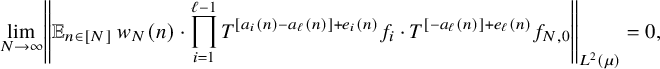 $$ \begin{align*} \lim_{N\to\infty} \left\Vert {\mathbb E}_{n\in [N]}\, w_{N}(n)\cdot \prod_{i=1}^{\ell-1} T^{[a_i(n)-a_\ell(n)]+e_i(n)}f_i\cdot T^{[-a_{\ell}(n)]+e_\ell(n)}f_{N,0}\right\Vert_{L^2(\mu)}=0, \end{align*} $$
for some $e_1(n),\ldots , e_{\ell -1}(n)\in \{0,1\}$
,
$e_1(n),\ldots , e_{\ell -1}(n)\in \{0,1\}$
, $n\in {\mathbb N}$
. Next, we would like to replace the error sequences
$n\in {\mathbb N}$
. Next, we would like to replace the error sequences $e_1,\ldots , e_{\ell -1}$
with constant sequences. To this end, we use Lemma 3.6 for I a singleton,
$e_1,\ldots , e_{\ell -1}$
with constant sequences. To this end, we use Lemma 3.6 for I a singleton, $J:=[N]$
,
$J:=[N]$
, $X:=L^\infty (\mu )$
,
$X:=L^\infty (\mu )$
, $A_N(n_1,\ldots ,n_\ell ):=\prod _{i=1}^{\ell -1} T^{n_i}f_i\cdot T^{-n_\ell }f_{N,0}$
,
$A_N(n_1,\ldots ,n_\ell ):=\prod _{i=1}^{\ell -1} T^{n_i}f_i\cdot T^{-n_\ell }f_{N,0}$
, $n_1,\ldots , n_\ell \in {\mathbb Z}$
, and
$n_1,\ldots , n_\ell \in {\mathbb Z}$
, and $b_i:=[a_i-a_{\ell }]$
,
$b_i:=[a_i-a_{\ell }]$
, $i=1,\ldots , \ell -1$
,
$i=1,\ldots , \ell -1$
, $b_\ell := [-a_\ell ]$
. We get that it suffices to show that
$b_\ell := [-a_\ell ]$
. We get that it suffices to show that
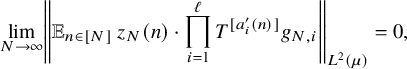 $$ \begin{align} \lim_{N\to\infty} \left\Vert {\mathbb E}_{n\in [N]}\, z_{N}(n)\cdot \prod_{i=1}^\ell T^{[a^{\prime}_i(n)]}g_{N,i}\right\Vert_{L^2(\mu)}=0, \end{align} $$
where
 $$ \begin{align*} a^{\prime}_i:=a_i-a_{\ell}, \quad i=1,\ldots, \ell-1, \quad a^{\prime}_\ell:= -a_\ell \end{align*} $$
for some $1$
-bounded sequence
$1$
-bounded sequence $(z_{N}(n))$
, where
$(z_{N}(n))$
, where $g_{N,i}:=T^{\epsilon _i}f_{i}$
,
$g_{N,i}:=T^{\epsilon _i}f_{i}$
, $i=1,\ldots , \ell -1$
,
$i=1,\ldots , \ell -1$
, $g_{N,\ell }:=T^{\epsilon _\ell }f_{N,0}$
,
$g_{N,\ell }:=T^{\epsilon _\ell }f_{N,0}$
, $N\in {\mathbb N}$
, for some constants
$N\in {\mathbb N}$
, for some constants $\epsilon _1,\ldots , \epsilon _\ell \in \{0,1\}$
. Note that the family
$\epsilon _1,\ldots , \epsilon _\ell \in \{0,1\}$
. Note that the family $a^{\prime }_1,\ldots , a^{\prime }_\ell $
is nice, and
$a^{\prime }_1,\ldots , a^{\prime }_\ell $
is nice, and $g_{N,1}=T^{\epsilon _1}f_1$
,
$g_{N,1}=T^{\epsilon _1}f_1$
, $N\in {\mathbb N}$
, so Theorem 3.1 applies (for
$N\in {\mathbb N}$
, so Theorem 3.1 applies (for $k=0$
and all but one of the functions independent of N) and gives that there exists
$k=0$
and all but one of the functions independent of N) and gives that there exists $s\in {\mathbb N}$
so that if
$s\in {\mathbb N}$
so that if $\lvert \!|\!| f_1|\!|\!\rvert _s=0$
, then equation (9) holds. This completes the proof.
$\lvert \!|\!| f_1|\!|\!\rvert _s=0$
, then equation (9) holds. This completes the proof.
We will prove Theorem 3.1 in Sections 4 and 5 using a PET-induction technique. The first section covers the base case of the induction where all the iterates have sublinear growth, and the subsequent section contains the proof of the induction step. Before moving into the details, we gather some basic tools that will be used in the argument.
3.2 Feedback from number theory
The next statement is well known and can be proved using elementary sieve theory methods (see, for example, [Reference Halberstam and Richert15, Theorem 5.7] or [Reference Iwaniec and Kowalski18, Theorem 6.7]).
Theorem 3.2. Let ${\mathbb P}$
be the set of prime numbers. For all
${\mathbb P}$
be the set of prime numbers. For all $k\in {\mathbb N}$
, there exist
$k\in {\mathbb N}$
, there exist $C_k>0$
such that for all distinct
$C_k>0$
such that for all distinct $h_1,\ldots , h_k\in {\mathbb N}$
and all
$h_1,\ldots , h_k\in {\mathbb N}$
and all $N\in {\mathbb N}$
, we have
$N\in {\mathbb N}$
, we have
 $$ \begin{align*} |\{n\in [N]\colon n+h_1,\ldots, n+h_k \in {\mathbb P}\}|\leq C_k\, \mathfrak{G}_k(h_1,\ldots, h_k)\, \frac{N}{(\log{N})^k}, \end{align*} $$
where
 $$ \begin{align} \mathfrak{G}_k(h_1,\ldots, h_k):=\prod_{p\in {\mathbb P}} \Big(1-\frac{1}{p}\Big)^{-k}\Big(1-\frac{\nu_p(h_1,\ldots, h_k)}{p}\Big) \end{align} $$
and $\nu _p(h_1,\ldots , h_k)$
denotes the number of congruence classes
$\nu _p(h_1,\ldots , h_k)$
denotes the number of congruence classes $\! \! \mod {p}$
that are occupied by
$\! \! \mod {p}$
that are occupied by $h_1,\ldots , h_k$
.
$h_1,\ldots , h_k$
.
We remark that although $\mathfrak {G}_1=1$
, the expression
$\mathfrak {G}_1=1$
, the expression $\mathfrak {G}_k(h_1,\ldots , h_k)$
is not bounded in
$\mathfrak {G}_k(h_1,\ldots , h_k)$
is not bounded in $h_1,\ldots , h_k$
if
$h_1,\ldots , h_k$
if $k\geq 2$
, and this causes some problems for us. Asymptotics for averages of powers of
$k\geq 2$
, and this causes some problems for us. Asymptotics for averages of powers of $\mathfrak {G}_k(h_1,\ldots , h_k)$
are given in [Reference Gallagher12] and [Reference Kowalski21, Theorem 1.1] using elementary but somewhat elaborate arguments. These results are not immediately applicable for our purposes, since we need to understand the behavior of
$\mathfrak {G}_k(h_1,\ldots , h_k)$
are given in [Reference Gallagher12] and [Reference Kowalski21, Theorem 1.1] using elementary but somewhat elaborate arguments. These results are not immediately applicable for our purposes, since we need to understand the behavior of $\mathfrak {G}_k$
on thin subsets of
$\mathfrak {G}_k$
on thin subsets of ${\mathbb Z}^k$
: for instance, when
${\mathbb Z}^k$
: for instance, when $k=4$
, we need to understand the averages of
$k=4$
, we need to understand the averages of $\mathfrak {G}_4(0,h_1,h_2,h_1+h_2)$
. Luckily, we only need to get upper bounds for these averages, and this can be done rather easily, as we will see shortly (a similar argument was used in [Reference Tao and Ziegler28] to handle averages over r of
$\mathfrak {G}_4(0,h_1,h_2,h_1+h_2)$
. Luckily, we only need to get upper bounds for these averages, and this can be done rather easily, as we will see shortly (a similar argument was used in [Reference Tao and Ziegler28] to handle averages over r of $\mathfrak {G}_k(0,r,2r,\ldots , (k-1)r)$
).
$\mathfrak {G}_k(0,r,2r,\ldots , (k-1)r)$
).
Definition. Let $\ell \in {\mathbb N}$
, and for
$\ell \in {\mathbb N}$
, and for ${\underline {h}}\in {\mathbb N}^\ell $
, let
${\underline {h}}\in {\mathbb N}^\ell $
, let $\text {Cube}({\underline {h}})\in {\mathbb N}^{2^\ell }$
be defined by
$\text {Cube}({\underline {h}})\in {\mathbb N}^{2^\ell }$
be defined by
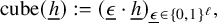 $$ \begin{align*} \text{cube}({\underline{h}}):=(\underline\epsilon\cdot {\underline{h}})_{\underline\epsilon\in\{0,1\}^\ell}, \end{align*} $$
where $\underline \epsilon \cdot {\underline {h}}$
is the inner product of
$\underline \epsilon \cdot {\underline {h}}$
is the inner product of $\underline \epsilon $
and
$\underline \epsilon $
and ${\underline {h}}$
.
${\underline {h}}$
.
If S is a subset of ${\mathbb N}^\ell $
, we define
${\mathbb N}^\ell $
, we define
 $$ \begin{align*} S^*:=\{{\underline{h}}\in S\colon \text{cube}({\underline{h}}) \text{ has distinct coordinates}\}. \end{align*} $$
For instance, when $\ell =3$
, we have
$\ell =3$
, we have
 $$ \begin{align*} \text{cube}(h_1,h_2,h_3)=(0,h_1,h_2,h_3,h_1+h_2, h_1+h_3,h_2+h_3,h_1+h_2+h_3), \end{align*} $$
and $([N]^3)^*$
consists of all triples
$([N]^3)^*$
consists of all triples $(h_1,h_2,h_3)\in [N]^3$
with distinct coordinates that in addition satisfy
$(h_1,h_2,h_3)\in [N]^3$
with distinct coordinates that in addition satisfy $h_i\neq h_j+h_k$
for all distinct
$h_i\neq h_j+h_k$
for all distinct $i,j,k\in \{1,2,3\}$
. Since the complement of
$i,j,k\in \{1,2,3\}$
. Since the complement of $([N]^\ell )^*$
in
$([N]^\ell )^*$
in $[N]^\ell $
is contained on the zero set of finitely many (at most
$[N]^\ell $
is contained on the zero set of finitely many (at most $3^\ell $
) linear forms, we get that there exists
$3^\ell $
) linear forms, we get that there exists $K_\ell>0$
such that
$K_\ell>0$
such that
 $$ \begin{align} |[N]^\ell\setminus ([N]^\ell)^*|\leq K_\ell\, N^{\ell-1} \end{align} $$
for every $N\in {\mathbb N}$
.
$N\in {\mathbb N}$
.
Proposition 3.3. For every $\ell \in {\mathbb N}$
, there exists
$\ell \in {\mathbb N}$
, there exists $C_\ell>0$
such that
$C_\ell>0$
such that
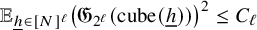 $$ \begin{align*} {\mathbb E}_{{\underline{h}} \in [N]^\ell} \big(\mathfrak{G}_{2^\ell}(\text{cube}({\underline{h}}) )\big)^2\leq C_\ell \end{align*} $$
for all $N\in {\mathbb N}$
, where
$N\in {\mathbb N}$
, where $\mathfrak {G}_{2^\ell }(\text {cube}({\underline {h}}))$
is as in equation (10).
$\mathfrak {G}_{2^\ell }(\text {cube}({\underline {h}}))$
is as in equation (10).
Remark. If we use kth powers instead of squares, we get similar upper bounds (which also depend on k), but we will not need this.
Proof. In the following argument, whenever we write p, we assume that p is a prime number.
Let ${\underline {h}}\in [N]^\ell $
. Note that if
${\underline {h}}\in [N]^\ell $
. Note that if $\nu _p(\text {cube}({\underline {h}}))=2^\ell $
, then
$\nu _p(\text {cube}({\underline {h}}))=2^\ell $
, then
 $$ \begin{align*} \Big(1-\frac{1}{p}\Big)^{-2^\ell}\Big(1-\frac{\nu_p(\text{cube}({\underline{h}}))}{p}\Big)\leq 1, \end{align*} $$
and if $\nu _p(\text {cube}({\underline {h}}))<2^\ell $
, then for
$\nu _p(\text {cube}({\underline {h}}))<2^\ell $
, then for $a_\ell :=2^{\ell +1}-2$
, we have
$a_\ell :=2^{\ell +1}-2$
, we have
 $$ \begin{align*} \Big(1-\frac{1}{p}\Big)^{-2^\ell}\Big(1-\frac{\nu_p(\text{cube}({\underline{h}}))}{p}\Big)\leq \Big(1-\frac{1}{p}\Big)^{-(2^\ell-1)}\leq e^{\frac{a_\ell}{p}}, \end{align*} $$
where we use that $\frac {1}{1-x}\leq e^{2x}$
for
$\frac {1}{1-x}\leq e^{2x}$
for $x\in [0,\frac {1}{2}]$
. Note also that if
$x\in [0,\frac {1}{2}]$
. Note also that if $\nu _p(\text {cube}({\underline {h}}))<2^\ell $
, then there exist distinct
$\nu _p(\text {cube}({\underline {h}}))<2^\ell $
, then there exist distinct $\underline \epsilon ,\underline \epsilon '\in \{0,1\}^{\ell }$
such that
$\underline \epsilon ,\underline \epsilon '\in \{0,1\}^{\ell }$
such that $p|(\underline \epsilon -\underline \epsilon ')\cdot {\underline {h}}$
, in which case we have that
$p|(\underline \epsilon -\underline \epsilon ')\cdot {\underline {h}}$
, in which case we have that $p\in \mathcal {P}({\underline {h}})$
, where
$p\in \mathcal {P}({\underline {h}})$
, where
 $$ \begin{align*} \mathcal{P}({\underline{h}}):=\bigcup_{\underline\epsilon,\underline\epsilon' \in \{0,1\}^\ell, \underline\epsilon,\neq \underline\epsilon' }\, \{p\in {\mathbb P} \colon p|(\underline\epsilon-\underline\epsilon')\cdot {\underline{h}}\}, \quad {\underline{h}}\in {\mathbb N}^\ell. \end{align*} $$
We deduce from the above facts and equation (10) that
 $$ \begin{align} \mathfrak{G}_{2^\ell}(\text{cube}({\underline{h}})) \leq e^{a_\ell \sum_{p\in \mathcal{P}({\underline{h}})}\frac{1}{p}}. \end{align} $$
By [Reference Tao and Ziegler27, Lemma E.1], we have for some $b_\ell ,c_\ell>0$
that
$b_\ell ,c_\ell>0$
that
 $$ \begin{align} e^{a_\ell \sum_{p\in \mathcal{P}({\underline{h}})}\frac{1}{p}} \leq b_\ell \sum_{p\in \mathcal{P}({\underline{h}})}\frac{(\log{p})^{c_\ell}}{p}= b_\ell \sum_{\underline\epsilon,\underline\epsilon' \in \{0,1\}^\ell, \underline\epsilon\neq \underline\epsilon'}\Big(\sum_{ p|(\underline\epsilon-\underline\epsilon')\cdot {\underline{h}}}\frac{(\log{p})^{c_\ell}}{p}\Big). \end{align} $$
Moreover, we get for some $d_\ell ,e_\ell>0$
that
$d_\ell ,e_\ell>0$
that
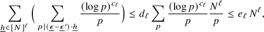 $$ \begin{align} \sum_{{\underline{h}}\in [N]^\ell}\Big(\sum_{ p|(\underline\epsilon-\underline\epsilon')\cdot {\underline{h}}}\frac{(\log{p})^{c_\ell}}{p}\Big)\leq d_\ell \sum_{ p}\frac{(\log{p})^{c_\ell}}{p} \frac{N^\ell}{p}\leq e_\ell\, N^\ell, \end{align} $$
for all $N\in {\mathbb N}$
, where to get the first estimate, we used the fact that for some
$N\in {\mathbb N}$
, where to get the first estimate, we used the fact that for some $d_\ell>0$
, we have
$d_\ell>0$
, we have
 $$ \begin{align*} |{\underline{h}}\in[N]^\ell\colon p|(\underline\epsilon-\underline\epsilon')\cdot {\underline{h}}|\leq d_\ell \frac{N^\ell}{p} \end{align*} $$
for all $N\in {\mathbb N}$
, and to get the second estimate, we used that
$N\in {\mathbb N}$
, and to get the second estimate, we used that $\sum _{ p}\frac {(\log {p})^{c_\ell }}{p^2}<\infty $
.
$\sum _{ p}\frac {(\log {p})^{c_\ell }}{p^2}<\infty $
.
If we take squares in equation (12), sum over all ${\underline {h}}\in [N]^\ell $
and then use equations (13) and (14), we get the asserted estimate.
${\underline {h}}\in [N]^\ell $
and then use equations (13) and (14), we get the asserted estimate.
From this we deduce the following estimate that is a crucial ingredient used in the proof of Theorem 2.4:
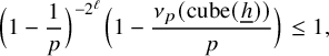
Corollary 3.4. Let $\ell \in {\mathbb N}$
. Then for every
$\ell \in {\mathbb N}$
. Then for every $A\geq 1$
, there exist
$A\geq 1$
, there exist $C_{A,\ell } ({\underline {h}})>0$
,
$C_{A,\ell } ({\underline {h}})>0$
, ${\underline {h}}\in {\mathbb N}^\ell $
and
${\underline {h}}\in {\mathbb N}^\ell $
and $D_{A,\ell }>0$
such that
$D_{A,\ell }>0$
such that
-
1. for all
$N\in {\mathbb N}$
,
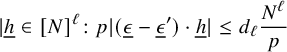
${\underline {h}}=(h_1,\ldots ,h_\ell )\in ({\mathbb N}^\ell )^*, c\in {\mathbb N},$
such that
$c+ h_1+\cdots +h_\ell \leq N^A$
, we have
$$ \begin{align*} {\mathbb E}_{n\in [N]}\, (\Delta_{\underline{h}} \Lambda')(n+c)\leq C_{A,\ell}({\underline{h}}); \end{align*} $$
-
2.
${\mathbb E}_{{\underline {h}}\in [H]^\ell } (C_{A,\ell }({\underline {h}}))^2\leq D_{A,\ell }$
for every
$H\in {\mathbb N}$
.


Remark. We will use this result in the proof of Lemma 4.1 for values of c that are larger than N and smaller than $N^A$
for some
$N^A$
for some $A>0$
(the choice of A depends on the situation).
$A>0$
(the choice of A depends on the situation).
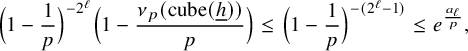
Proof. Since $\Lambda '$
is supported on primes and
$\Lambda '$
is supported on primes and $c+h_1+\cdots +h_\ell \leq N^A$
, we have that
$c+h_1+\cdots +h_\ell \leq N^A$
, we have that
 $$ \begin{align*} \sum_{n\in [N]}\, (\Delta_{\underline{h}}\Lambda')(n+c)\leq |\{n\in [N]\colon \underline{n+c}+\text{cube}({\underline{h}})\in {\mathbb P}^{2^\ell}\}|\cdot (\log(N+N^A))^{2^\ell}, \end{align*} $$
where $\underline {n+c}$
is a vector with
$\underline {n+c}$
is a vector with $2^\ell $
coordinates, all equal to
$2^\ell $
coordinates, all equal to $n+c$
. Note that for
$n+c$
. Note that for ${\underline {h}}\in ({\mathbb N}^\ell )^*$
, we can apply Theorem 3.2, and we get that there exists
${\underline {h}}\in ({\mathbb N}^\ell )^*$
, we can apply Theorem 3.2, and we get that there exists $D_{A,\ell }>0$
such that for every
$D_{A,\ell }>0$
such that for every $N\in {\mathbb N}$
, the last expression is bounded by
$N\in {\mathbb N}$
, the last expression is bounded by
 $$ \begin{align*} D_{A,\ell}\, \mathfrak{G}_{2^\ell}(\text{cube}({\underline{h}}))\, N. \end{align*} $$
If we let $C_{A,\ell }({\underline {h}}):=D_{A,\ell }\, \mathfrak {G}_{2^\ell }(\text {cube}({\underline {h}}))$
and
$C_{A,\ell }({\underline {h}}):=D_{A,\ell }\, \mathfrak {G}_{2^\ell }(\text {cube}({\underline {h}}))$
and ${\underline {h}}\in {\mathbb N}^\ell $
and use Proposition 3.3, we get that properties
${\underline {h}}\in {\mathbb N}^\ell $
and use Proposition 3.3, we get that properties $(i)$
and
$(i)$
and $(ii)$
hold.
$(ii)$
hold.
3.3 Two elementary lemmas
We will use the following inner product space variant of a classical elementary estimate of van der Corput (see [Reference Kuipers and Niederreiter22, Lemma 3.1]):
Lemma 3.5. Let $N\in {\mathbb N}$
and
$N\in {\mathbb N}$
and $(u(n))_{n\in [N]}$
be vectors in some inner product space. Then for all
$(u(n))_{n\in [N]}$
be vectors in some inner product space. Then for all $H\in [N]$
, we have
$H\in [N]$
, we have
 $$ \begin{align*} \left\Vert {\mathbb E}_{n\in [N]}\, u(n)\right\Vert^2\leq \frac{2}{H}\, {\mathbb E}_{n\in [N]}\left\Vert u(n)\right\Vert^2 + 4\, {\mathbb E}_{h\in[H]}\Big(1-\frac{h}{H}\Big)\Re\Big(\frac{1}{N}\sum_{n=1}^{N-h} \langle u(n+h),u(n)\rangle \Big). \end{align*} $$
We will apply the previous lemma in the following two cases, depending on the range of the shift parameter h (the first case will be used when the relevant sequences are not necessarily bounded).
-
1. If
$M_N:=1+\max _{n\in [N]}\left \Vert u_N(n)\right \Vert {}^2$
,
$N\in {\mathbb N}$
and
$L_N$
are such that
$M_N\prec L_N\prec \frac {N}{M_N}$
, then for
$H:=L_N$
, we have (15)where for every fixed
$$ \begin{align} \left\Vert {\mathbb E}_{n\in [N]} \, u_N(n)\right\Vert^2\leq 4\, {\mathbb E}_{h\in [L_N]} \Big|{\mathbb E}_{n\in[N]}\langle u_N(n+h), u_N(n)\rangle \Big| +o_N(1), \end{align} $$
$N\in {\mathbb N}$
, the sequence
$(u_N(n))$
is either defined on the larger interval
$[N+L_N]$
or extended to be zero outside the interval
$[N]$
. In all the cases where we will apply this estimate, we have
$M_N\ll (\log N)^A$
for some
$A>0$
, and we take
$L_N=[e^{\sqrt {\log {N}} }]$
,
$N\in {\mathbb N}$
.
-
2. If the sequence
$(u_N(n))$
is bounded, then we have (16)where for every fixed
$$ \begin{align} \limsup_{N\to\infty} \left\Vert {\mathbb E}_{n\in [N]}\, u_N(n)\right\Vert^2\leq 4\, \limsup_{H\to\infty} {\mathbb E}_{h\in [H]} \limsup_{N\to\infty}\Big|{\mathbb E}_{n\in[N]}\langle u_N(n+h), u_N(n)\rangle \Big|, \end{align} $$
$N\in {\mathbb N}$
, the sequence
$(u_N(n))$
is either defined on the larger interval
$[N+H]$
or extended to be zero outside the interval
$[N]$
.


We will also make frequent use of the following simple lemma, or variants of it, to replace error sequences that take finitely many integer values with constant sequences.
Lemma 3.6. For $f,\ell \in {\mathbb N}$
, there exists
$f,\ell \in {\mathbb N}$
, there exists $C_{f,\ell }>0$
such that the following holds: Let
$C_{f,\ell }>0$
such that the following holds: Let $(X,\left \Vert \cdot \right \Vert )$
be a normed space and F be a finite subset of
$(X,\left \Vert \cdot \right \Vert )$
be a normed space and F be a finite subset of ${\mathbb Z}$
with
${\mathbb Z}$
with $|F|=f$
,
$|F|=f$
, $k\in {\mathbb N}$
, and
$k\in {\mathbb N}$
, and $I\subset {\mathbb N}^k$
,
$I\subset {\mathbb N}^k$
, $J\subset {\mathbb N}$
be finite. For
$J\subset {\mathbb N}$
be finite. For ${\underline {h}}\in I$
, consider sequences
${\underline {h}}\in I$
, consider sequences $A_{\underline {h}}\colon {\mathbb Z}^\ell \to X$
,
$A_{\underline {h}}\colon {\mathbb Z}^\ell \to X$
, $b_{1,{\underline {h}}},\ldots , b_{\ell ,{\underline {h}}}\colon J\to {\mathbb Z}$
,
$b_{1,{\underline {h}}},\ldots , b_{\ell ,{\underline {h}}}\colon J\to {\mathbb Z}$
, $w_{\underline {h}} \colon J\to {\mathbb C}$
, and
$w_{\underline {h}} \colon J\to {\mathbb C}$
, and $e_{1,{\underline {h}}},\ldots , e_{\ell ,{\underline {h}}}\colon J\to F$
. Then there exist sequences
$e_{1,{\underline {h}}},\ldots , e_{\ell ,{\underline {h}}}\colon J\to F$
. Then there exist sequences $\tilde {w}_{\underline {h}}\colon J\to {\mathbb C}$
,
$\tilde {w}_{\underline {h}}\colon J\to {\mathbb C}$
, ${\underline {h}}\in I$
, with
${\underline {h}}\in I$
, with $\left \Vert \tilde {w}_{\underline {h}}\right \Vert {}_{L^\infty (J)}\leq \left \Vert w_{\underline {h}}\right \Vert {}_{L^\infty (J)}$
and constants
$\left \Vert \tilde {w}_{\underline {h}}\right \Vert {}_{L^\infty (J)}\leq \left \Vert w_{\underline {h}}\right \Vert {}_{L^\infty (J)}$
and constants $\epsilon _1,\ldots , \epsilon _\ell \in F$
, such that
$\epsilon _1,\ldots , \epsilon _\ell \in F$
, such that
 $$ \begin{align*} \sum_{{\underline{h}}\in I} \Big|\Big|\sum_{n\in J}\, w_{\underline{h}}(n)\cdot A_{{\underline{h}}}(b_{1,{\underline{h}}}(n)+e_{1,{\underline{h}}}&(n),\ldots, b_{\ell,{\underline{h}}}(n)+e_{\ell,{\underline{h}}}(n)) \Big|\Big| \leq \\ &C_{f,\ell}\, \sum_{{\underline{h}}\in I}\Big|\Big|\sum_{n\in J} \,\tilde{w}_{\underline{h}}(n)\cdot A_{\underline{h}}(b_{1,{\underline{h}}}(n)+\epsilon_1,\ldots, b_{\ell,{\underline{h}}}(n)+\epsilon_\ell)\Big|\Big|. \end{align*} $$
Remark. Often, when this estimate is used, the sequence $A_{\underline {h}}$
is defined only on a subset of
$A_{\underline {h}}$
is defined only on a subset of ${\mathbb Z}^\ell $
, and we assume that it is extended to be zero at the elements where it is not defined.
${\mathbb Z}^\ell $
, and we assume that it is extended to be zero at the elements where it is not defined.
Proof. The expression on the left-hand side is bounded by
 $$ \begin{align*} \sum_{j=1}^t\sum_{{\underline{h}}\in I} \Big|\Big|\sum_{n\in J}\, w_{\underline{h}}(n)\cdot A_{\underline{h}}(b_{1,{\underline{h}}}(n)+e_{1,{\underline{h}}}(n),\ldots, b_{\ell,{\underline{h}}}(n)+e_{\ell,{\underline{h}}}(n)) \cdot \mathbf{1}_{E_{j,{\underline{h}}}} (n)\Big|\Big|, \end{align*} $$
where for $t=f^\ell $
, the sets
$t=f^\ell $
, the sets $E_{1,{\underline {h}}},\ldots , E_{t,{\underline {h}}}$
form a partition of
$E_{1,{\underline {h}}},\ldots , E_{t,{\underline {h}}}$
form a partition of ${\mathbb N}$
into sets (possibly empty) on which all the sequences
${\mathbb N}$
into sets (possibly empty) on which all the sequences $e_{1,{\underline {h}}},\ldots , e_{\ell ,{\underline {h}}}$
are constant (and the constants do not depend on
$e_{1,{\underline {h}}},\ldots , e_{\ell ,{\underline {h}}}$
are constant (and the constants do not depend on ${\underline {h}}$
). If the maximum of the summands over j occurs for some
${\underline {h}}$
). If the maximum of the summands over j occurs for some $j_0\in [t]$
, then there exist
$j_0\in [t]$
, then there exist $\epsilon _1,\ldots , \epsilon _\ell \in F$
such that for all
$\epsilon _1,\ldots , \epsilon _\ell \in F$
such that for all $n\in E_{j_0, {\underline {h}}}$
, we have
$n\in E_{j_0, {\underline {h}}}$
, we have $e_{i,{\underline {h}}}(n)=\epsilon _i$
,
$e_{i,{\underline {h}}}(n)=\epsilon _i$
, $i \in [\ell ]$
,
$i \in [\ell ]$
, ${\underline {h}} \in I$
. Hence, the last sum is bounded by
${\underline {h}} \in I$
. Hence, the last sum is bounded by
 $$ \begin{align*} t \sum_{{\underline{h}}\in I}\Big|\Big|\sum_{n\in J}\, \tilde{w}_{\underline{h}}(n)\cdot A_{\underline{h}}(b_{1,{\underline{h}}}(n)+\epsilon_1,\ldots, b_{\ell,{\underline{h}}}(n)+\epsilon_\ell) \Big|\Big|, \end{align*} $$
where $\tilde {w}_{\underline {h}}(n):=w_{\underline {h}}(n)\cdot \mathbf {1}_{E_{j_0,{\underline {h}}}}(n)$
,
$\tilde {w}_{\underline {h}}(n):=w_{\underline {h}}(n)\cdot \mathbf {1}_{E_{j_0,{\underline {h}}}}(n)$
, $n\in J$
,
$n\in J$
, ${\underline {h}}\in I$
.
${\underline {h}}\in I$
.
We will use the previous lemma to handle some error sequences that occur when we use the Taylor expansion in order to perform some approximations and when we replace the sum (or the difference) of the integer parts of sequences with the corresponding integer part of their sum (or the difference), and vice versa. For instance, if $e_1(n),\ldots e_\ell (n)\in (-1,1)$
,
$e_1(n),\ldots e_\ell (n)\in (-1,1)$
, $n\in [N]$
, we have
$n\in [N]$
, we have
 $$ \begin{align*} &\left\Vert {\mathbb E}_{n\in [N]}\, w(n)\cdot A([a_1(n)+b_1(n)+e_1(n)],\ldots, [a_\ell(n)+b_\ell(n)+e_\ell(n)])\right\Vert\leq \\ &\qquad\quad\qquad\qquad\qquad 4^\ell\, \left\Vert {\mathbb E}_{n\in [N]}\, \tilde{w}(n)\cdot A([a_1(n)]+[b_1(n)]+\epsilon_1,\ldots, [a_\ell(n)]+[b_\ell(n)]+\epsilon_\ell)\right\Vert \end{align*} $$
for some $\epsilon _1,\ldots , \epsilon _\ell \in \{-1,0,1,2\}$
and
$\epsilon _1,\ldots , \epsilon _\ell \in \{-1,0,1,2\}$
and $\tilde {w}\colon [N]\to {\mathbb C}$
with
$\tilde {w}\colon [N]\to {\mathbb C}$
with $\left \Vert \tilde {w}\right \Vert {}_{L^\infty [N]}\leq \left \Vert w\right \Vert {}_{L^\infty [N]}$
. Often the constants
$\left \Vert \tilde {w}\right \Vert {}_{L^\infty [N]}\leq \left \Vert w\right \Vert {}_{L^\infty [N]}$
. Often the constants $\epsilon _1,\ldots , \epsilon _\ell $
make no difference for our argument and can be ignored.
$\epsilon _1,\ldots , \epsilon _\ell $
make no difference for our argument and can be ignored.
4 Seminorm estimates – sublinear case
The goal of this section is to establish Theorem 3.1 in the case where all the iterates have fractional degree smaller than $1$
; see Proposition 4.4 below.
$1$
; see Proposition 4.4 below.
4.1 An example
We explain in some detail how the proof of Theorem 3.1 works when $k=1, \ell =2$
and
$k=1, \ell =2$
and $a_1(h,t):=p_1(h)t^{0.5}+q_1(h)t^{0.1}$
,
$a_1(h,t):=p_1(h)t^{0.5}+q_1(h)t^{0.1}$
, $a_2(h,t):=p_2(h)t^{0.5}+q_2(h)t^{0.1}$
,
$a_2(h,t):=p_2(h)t^{0.5}+q_2(h)t^{0.1}$
, $h\in {\mathbb N}$
,
$h\in {\mathbb N}$
, $t\in {\mathbb R}_+$
. We assume that
$t\in {\mathbb R}_+$
. We assume that $p_1\neq 0$
and
$p_1\neq 0$
and $a_1, a_2, a_1-a_2$
are nonzero.
$a_1, a_2, a_1-a_2$
are nonzero.
We also assume that the sequence of weights $(w_{N,h}(n))$
is defined by
$(w_{N,h}(n))$
is defined by
 $$ \begin{align*} w_{N,h}(n):=\Lambda'(n)\cdot \Lambda'(n+h)\cdot c_{N,h}(n), \quad h\in [L_N],\, n\in[N],\, N\in {\mathbb N}, \end{align*} $$
where $(c_{N,h}(n))$
is a
$(c_{N,h}(n))$
is a $1$
-bounded sequence.
$1$
-bounded sequence.
Our aim is to show that there exists $s\in {\mathbb N}$
such that if
$s\in {\mathbb N}$
such that if $\lvert \!|\!| f_1|\!|\!\rvert _s=0$
, then
$\lvert \!|\!| f_1|\!|\!\rvert _s=0$
, then
 $$ \begin{align*} \lim_{N\to\infty} {\mathbb E}_{h\in [L_N]}\left\Vert {\mathbb E}_{n\in [N]}\, w_{N,h}(n) \cdot \prod_{i=1}^2T^{[p_i(h)n^{0.5}+q_i(h)n^{0.1}]}f_i\right\Vert_{L^2(\mu)}=0. \end{align*} $$
Step 1. Our first goal is to use the number theory feedback of Section 3.2 to reduce matters to showing mean convergence to zero for some other averages with bounded weights $w_{N,h}$
(this step corresponds to Lemma 4.1 below). We let
$w_{N,h}$
(this step corresponds to Lemma 4.1 below). We let
 $$ \begin{align*} p(h):=[\max\{|p_1|(h),|p_2|(h),|q_1|(h),|q_2|(h)\}^{10}]+1, \quad h\in{\mathbb N}.\\[-15pt] \end{align*} $$
Note that p is not a polynomial, but this will not bother us. After splitting the average over $[N]$
into subintervals, we see (this reduction will be explained in more detail in the proof of Lemma 4.1) that it suffices to show mean convergence to zero for
$[N]$
into subintervals, we see (this reduction will be explained in more detail in the proof of Lemma 4.1) that it suffices to show mean convergence to zero for
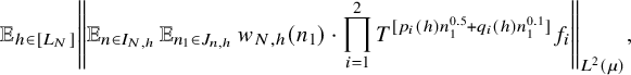 $$ \begin{align*} {\mathbb E}_{h\in [L_N]}\left\Vert {\mathbb E}_{n\in I_{N,h}}\, {\mathbb E}_{n_1\in J_{n,h}} \, w_{N,h}(n_1) \cdot \prod_{i=1}^2 T^{[p_i(h)n_1^{0.5}+q_i(h)n_1^{0.1}]}f_i\right\Vert_{L^2(\mu)},\\[-15pt] \end{align*} $$
where
 $$ \begin{align*} I_{N,h}:= [N^{0.5}p(h)], \quad J_{n,h}:=\Big[\Big(\frac{n-1}{p(h)}\Big)^2,\Big(\frac{n}{p(h)}\Big)^2\Big), \quad n\in I_{N,h}, \, h\in [L_N], \, N\in{\mathbb N}.\\[-15pt] \end{align*} $$
For convenience, we write
 $$ \begin{align*} J_{n,h}=(k_{n,h},k_{n,h}+l_{n,h}] , \quad n\in I_{N,h}, \, h\in [L_N], \, N\in{\mathbb N}\\[-15pt] \end{align*} $$
for some $k_{n,h}, l_{n,h}\in {\mathbb N}$
.
$k_{n,h}, l_{n,h}\in {\mathbb N}$
.
Note that for fixed $n,h\in {\mathbb N}$
, when
$n,h\in {\mathbb N}$
, when $n_1$
ranges in
$n_1$
ranges in $J_{n,h}$
, the value of
$J_{n,h}$
, the value of $p_1(h)n_1^{0.5}$
ranges in an interval of length at most
$p_1(h)n_1^{0.5}$
ranges in an interval of length at most $1$
; the same property holds for the values of
$1$
; the same property holds for the values of $p_2(h)n_1^{0.5}$
,
$p_2(h)n_1^{0.5}$
, $q_1(h)n_1^{0.1}$
,
$q_1(h)n_1^{0.1}$
, $q_2(h)n_1^{0.1}$
. Hence, for
$q_2(h)n_1^{0.1}$
. Hence, for $n_1\in J_{n,h}$
, we have
$n_1\in J_{n,h}$
, we have
 $$ \begin{align*} p_i(h)n_1^{0.5}+q_i(h)n_1^{0.1}=\frac{p_i(h)}{p(h)}n+q_i(h)\Big(\frac{n}{p(h)}\Big)^{0.2}+e_i(h,n,n_1),\quad i=1,2,\\[-15pt] \end{align*} $$
where $e_1(h,n,n_1) , e_2(h,n,n_1)$
are bounded by
$e_1(h,n,n_1) , e_2(h,n,n_1)$
are bounded by $2$
for all
$2$
for all $n_1\in J_{n,h}$
,
$n_1\in J_{n,h}$
, $n\in I_{N,h}$
,
$n\in I_{N,h}$
, $h\in [L_N]$
,
$h\in [L_N]$
, $N\in {\mathbb N}$
. Using Lemma 3.6, and since replacing
$N\in {\mathbb N}$
. Using Lemma 3.6, and since replacing $f_i$
with
$f_i$
with $T^{\epsilon _{i,N}}f_i$
,
$T^{\epsilon _{i,N}}f_i$
, $i=1,2$
, where
$i=1,2$
, where $\epsilon _{1,N}, \epsilon _{2,N}$
take finitely many values for
$\epsilon _{1,N}, \epsilon _{2,N}$
take finitely many values for $N\in {\mathbb N}$
, does not introduce changes to our argument, we can ignore these error terms. We are thus left with showing convergence to zero for
$N\in {\mathbb N}$
, does not introduce changes to our argument, we can ignore these error terms. We are thus left with showing convergence to zero for
 $$ \begin{align*} {\mathbb E}_{h\in [L_N]}\left\Vert {\mathbb E}_{n\in I_{N,h}}\, \tilde{w}_{N,h}(n) \cdot \prod_{i=1}^2 T^{\big[\frac{p_i(h)}{p(h)}n+q_i(h) (\frac{n}{p(h)})^{0.2}\big]}f_i\right\Vert_{L^2(\mu)},\\[-15pt] \end{align*} $$
where for $n\in [I_{N,h}]$
,
$n\in [I_{N,h}]$
, $h\in [L_N]$
,
$h\in [L_N]$
, $N\in {\mathbb N}$
, we let
$N\in {\mathbb N}$
, we let
 $$ \begin{align} \tilde{w}_{N,h}(n):= {\mathbb E}_{n_1\in J_{n,h}} \, w_{N,h}(n_1) = {\mathbb E}_{n_1\in [l_{n,h}]} \, \Lambda'(n_1+k_{n,h})\cdot \Lambda'(n_1+k_{n,h}+h)\cdot c_{N,h}(n_1+k_{n,h}).\\[-15pt]\nonumber \end{align} $$
From the definition of $k_{n,h}$
,
$k_{n,h}$
, $l_{n,h}$
,
$l_{n,h}$
, $L_N$
, we get that there exists
$L_N$
, we get that there exists $N_0=N_0(p)\in {\mathbb N}$
such that
$N_0=N_0(p)\in {\mathbb N}$
such that
 $$ \begin{align*} k_{n,h}+h\leq l_{n,h}^3, \quad \text{for all } n\in [N^{0.4},N^{0.5}p(h)], \, h\in [L_N], \, N\geq N_0.\\[-15pt] \end{align*} $$
Using Corollary 3.4 (with $\ell =1$
,
$\ell =1$
, $A=3$
,
$A=3$
, $c=k_{n,h}$
,
$c=k_{n,h}$
, $N=l_{n,h}$
), we see that there exist
$N=l_{n,h}$
), we see that there exist $D>0$
and
$D>0$
and $C(h)$
,
$C(h)$
, $h\in {\mathbb N}$
, such that for the above-mentioned values of
$h\in {\mathbb N}$
, such that for the above-mentioned values of $n,h,N$
, we can write
$n,h,N$
, we can write
 $$ \begin{align*} \tilde{w}_{N,h}(n)=C(h)\cdot z_{N,h}(n), \end{align*} $$
where $(z_{N,h}(n))$
is
$(z_{N,h}(n))$
is $1$
-bounded and
$1$
-bounded and
 $$ \begin{align*} {\mathbb E}_{h\in[L_N]}(C(h))^2\leq D \end{align*} $$
for every $N\in {\mathbb N}$
.
$N\in {\mathbb N}$
.
We use this estimate, apply the Cauchy-Schwarz inequality and keep in mind that the part of the intervals $I_{N,h}$
that intersects the interval
$I_{N,h}$
that intersects the interval $[N^{0.4}]$
is negligible for our averages. We deduce that it suffices to show convergence to zero for
$[N^{0.4}]$
is negligible for our averages. We deduce that it suffices to show convergence to zero for
 $$ \begin{align*} {\mathbb E}_{h\in [L_N]}\left\Vert {\mathbb E}_{n\in I_{N,h}}\, z_{N,h}(n) \cdot \prod_{i=1}^2 T^{\big[\frac{p_i(h)}{p(h)}n+q_i(h)(\frac{n}{p(h)})^{0.2}\big]}f_i\right\Vert^2_{L^2(\mu)}, \end{align*} $$
where the sequence $(z_{N,h}(n))$
is
$(z_{N,h}(n))$
is $1$
-bounded. We write
$1$
-bounded. We write $n=n'p(h)+s$
for some
$n=n'p(h)+s$
for some $n'\in [N^{0.5}]$
and
$n'\in [N^{0.5}]$
and $s\in [p(h)]$
. For convenience, we also rename
$s\in [p(h)]$
. For convenience, we also rename $n'$
as n and use Lemma 3.6 to treat finite valued error sequences that are introduced when we approximate
$n'$
as n and use Lemma 3.6 to treat finite valued error sequences that are introduced when we approximate $q_i(h)(n+s/p(h))^{0.2}$
with
$q_i(h)(n+s/p(h))^{0.2}$
with $q_i(h)n^{0.2}$
,
$q_i(h)n^{0.2}$
, $i=1,2$
. We get that it suffices to show convergence to zero for
$i=1,2$
. We get that it suffices to show convergence to zero for
 $$ \begin{align*} {\mathbb E}_{h\in [L_N]}{\mathbb E}_{s\in [p(h)]}\left\Vert {\mathbb E}_{n\in [N^{0.5}]}\, z_{N,h,s}(n) \cdot \prod_{i=1}^2 T^{[p_i(h)n+q_i(h)n^{0.2}+e_i(h,s)]}f_i\right\Vert^2_{L^2(\mu)}, \end{align*} $$
where $(z_{N,h,s}(n))$
is some other
$(z_{N,h,s}(n))$
is some other $1$
-bounded sequence and
$1$
-bounded sequence and $e_i(h,s):=s\frac {p_i(h)}{p(h)}$
,
$e_i(h,s):=s\frac {p_i(h)}{p(h)}$
, $i=1,2$
. After replacing the average
$i=1,2$
. After replacing the average ${\mathbb E}_{s\in [p(h)]}$
with
${\mathbb E}_{s\in [p(h)]}$
with $\max _{s\in [p(h)]}$
, we are left with dealing with the averages
$\max _{s\in [p(h)]}$
, we are left with dealing with the averages
 $$ \begin{align*} {\mathbb E}_{h\in [L_N]}\left\Vert {\mathbb E}_{n\in [N^{0.5}]}\, z_{N,h}(n) \cdot \prod_{i=1}^2 T^{[p_i(h)n+q_i(h)n^{0.2} +e_{i,N}(h)]}f_i \right\Vert^2_{L^2(\mu)} \end{align*} $$
for some other $1$
-bounded sequence
$1$
-bounded sequence $(z_{N,h}(n))$
and arbitrary sequences of real numbers
$(z_{N,h}(n))$
and arbitrary sequences of real numbers $(e_{1,N}(h)), (e_{2,N}(h))$
(which will be eliminated later, so their particular form is not important).
$(e_{1,N}(h)), (e_{2,N}(h))$
(which will be eliminated later, so their particular form is not important).
Step 2. Our next goal is to reduce matters to showing mean convergence to zero for averages with iterates given by polynomials in several variables and real coefficients (this step corresponds to Lemma 4.2 below). After using equation (15) for the average over n, we are left with showing convergence to zero for
 $$ \begin{align*} {\mathbb E}_{h,h_1\in [L_N]}\Big|{\mathbb E}_{n\in [N^{0.5}]}\, c_{N,h,h_1}(n)&\cdot \int \prod_{i=1}^2 T^{[p_i(h)(n+h_1)+q_i(h)(n+h_1)^{0.2} +e_{i,N}(h)]}f_i\cdot \\ &\qquad\qquad\qquad\qquad\qquad\qquad\prod_{i=1}^2 T^{[p_i(h)n+q_i(h)n^{0.2} +e_{i,N}(h)]}\overline{f}_i\, d\mu\Big|, \end{align*} $$
where $(c_{N,h,h_1}(n))$
is a
$(c_{N,h,h_1}(n))$
is a $1$
-bounded sequence. We compose with
$1$
-bounded sequence. We compose with $T^{-[p_2(h)n+q_2(h)n^{0.2} +e_{2,N}(h)]}$
(and not with
$T^{-[p_2(h)n+q_2(h)n^{0.2} +e_{2,N}(h)]}$
(and not with $T^{-[p_1(h)n+q_1(h)n^{0.2} +e_{1,N}(h)]}$
because we want the highest fractional degree iterate to be applied to the function
$T^{-[p_1(h)n+q_1(h)n^{0.2} +e_{1,N}(h)]}$
because we want the highest fractional degree iterate to be applied to the function $f_1$
), use that
$f_1$
), use that $(n+h_1)^{0.2}$
can for our purposes be replaced with
$(n+h_1)^{0.2}$
can for our purposes be replaced with $n^{0.2}$
, ignore errors that take finitely many values using Lemma 3.6 and use the Cauchy-Schwarz inequality. We are left with showing convergence to zero for
$n^{0.2}$
, ignore errors that take finitely many values using Lemma 3.6 and use the Cauchy-Schwarz inequality. We are left with showing convergence to zero for
 $$ \begin{align*} {\mathbb E}_{h,h_1\in [L_N]}\left\Vert {\mathbb E}_{n\in [N^{0.5}]}\, c_{N,h,h_1}(n) \cdot T^{[(p_1-p_2)(h)n+(q_1-q_2)(h)n^{0.2} +e_{3,N}(h)]} (T^{[p_1(h)h_1]}f_1\cdot \overline{f}_1)\right\Vert_{L^2(\mu)}, \end{align*} $$
where $ (c_{N,h,h_1}(n))$
is some other
$ (c_{N,h,h_1}(n))$
is some other $1$
-bounded sequence and the sequence
$1$
-bounded sequence and the sequence $(e_{3,N}(h))$
takes arbitrary real values.
$(e_{3,N}(h))$
takes arbitrary real values.
We consider two cases. Suppose first that $p_1=p_2$
. Then by assumption,
$p_1=p_2$
. Then by assumption, $q_1-q_2\neq 0$
. Repeating the argument used in Step 1, we are left with showing convergence to zero for
$q_1-q_2\neq 0$
. Repeating the argument used in Step 1, we are left with showing convergence to zero for
 $$ \begin{align*} {\mathbb E}_{h,h_1\in [L_N]}\left\Vert {\mathbb E}_{n\in [N^{0.1}]}\, c_{N,h,h_1}(n) \cdot T^{[(q_1-q_2)(h)n +e_{4,N}(h)]} (T^{[p_1(h)h_1]}f_1\cdot \overline{f}_1)\right\Vert_{L^2(\mu)} \end{align*} $$
for some other $1$
-bounded sequence of complex numbers
$1$
-bounded sequence of complex numbers $(c_{N,h,h_1}(n))$
and
$(c_{N,h,h_1}(n))$
and $(e_{4,N}(h))$
arbitrary sequence of real numbers. Using as above equation (15) for the average over n, composing with
$(e_{4,N}(h))$
arbitrary sequence of real numbers. Using as above equation (15) for the average over n, composing with $T^{-[(q_1-q_2)(h)n +e_{4,N}(h)]}$
and then using the Cauchy-Schwarz inequality and Lemma 3.6 to treat errors, we are left with showing mean convergence to zero for
$T^{-[(q_1-q_2)(h)n +e_{4,N}(h)]}$
and then using the Cauchy-Schwarz inequality and Lemma 3.6 to treat errors, we are left with showing mean convergence to zero for
 $$ \begin{align*} {\mathbb E}_{h,h_1,h_2\in [L_N]}\, c_{N,h,h_1,h_2}(n)\cdot T^{[(q_1-q_2)(h)h_2+p_1(h)h_1]}f_1\cdot T^{[(q_1-q_2)(h)h_2]}\overline{f}_1 \cdot T^{[p_1(h)h_1]}\overline{f}_1 \end{align*} $$
for some $1$
-bounded sequence of complex numbers
$1$
-bounded sequence of complex numbers $(c_{N,h,h_1, h_2}(n))$
.
$(c_{N,h,h_1, h_2}(n))$
.
If $p_1\neq p_2$
, we apply equation (15) for the average over n, compose with the transformation
$p_1\neq p_2$
, we apply equation (15) for the average over n, compose with the transformation $T^{-[(p_1-p_2)(h)n+(q_1-q_2)(h)n^{0.2} +e_{3,N}(h)]}$
and use the Cauchy-Schwarz inequality and Lemma 3.6 to treat errors. We are left with showing mean convergence to zero for
$T^{-[(p_1-p_2)(h)n+(q_1-q_2)(h)n^{0.2} +e_{3,N}(h)]}$
and use the Cauchy-Schwarz inequality and Lemma 3.6 to treat errors. We are left with showing mean convergence to zero for
 $$ \begin{align*} {\mathbb E}_{h,h_1,h_2\in [L_N]}\, c_{N,h,h_1,h_2}(n) \cdot T^{[(p_1-p_2)(h)h_2+p_1(h)h_1]}f_1\cdot T^{[(p_1-p_2)(h)h_2]}\overline{f}_1 \cdot T^{[p_1(h)h_1]}\overline{f}_1 \end{align*} $$
for some other $1$
-bounded sequence of complex numbers
$1$
-bounded sequence of complex numbers $(c_{N,h,h_1, h_2}(n))$
.
$(c_{N,h,h_1, h_2}(n))$
.
Step 3. In Step 2, we were led to show mean convergence to zero for averages with iterates given by nonconstant polynomials with real coefficients in several variables that have pairwise nonconstant differences. For such averages, one can argue as in [Reference Leibman23] to show that there exists $s\in {\mathbb N}$
such that if
$s\in {\mathbb N}$
such that if $\lvert \!|\!| f_1|\!|\!\rvert _s=0$
, then we have mean convergence to zero. For more details, see the proof of Lemma 4.3 below. This achieves our goal.
$\lvert \!|\!| f_1|\!|\!\rvert _s=0$
, then we have mean convergence to zero. For more details, see the proof of Lemma 4.3 below. This achieves our goal.
4.2 Reduction to averages with bounded weights and change of variables
Our first goal is to prove the following result that allows us to restrict to the case where the weights $w_{N,{\underline {h}}}$
are
$w_{N,{\underline {h}}}$
are $1$
-bounded and also allows us to perform the substitution
$1$
-bounded and also allows us to perform the substitution $n\mapsto n^{1/d}$
.
$n\mapsto n^{1/d}$
.
Lemma 4.1. For $k\in {\mathbb Z}_+,\ell \in {\mathbb N}$
, let
$k\in {\mathbb Z}_+,\ell \in {\mathbb N}$
, let $a_1,\ldots , a_\ell $
be a nice collection of fractional polynomials with k-parameters and suppose that
$a_1,\ldots , a_\ell $
be a nice collection of fractional polynomials with k-parameters and suppose that $d:=\text {f-deg}(a_1)\in (0,1)$
. Then the following holds: If
$d:=\text {f-deg}(a_1)\in (0,1)$
. Then the following holds: If $(X,\mu ,T)$
is a system,
$(X,\mu ,T)$
is a system, $f_{N,{\underline {h}},1},\ldots , f_{N,{\underline {h}},\ell }\in L^\infty (\mu )$
,
$f_{N,{\underline {h}},1},\ldots , f_{N,{\underline {h}},\ell }\in L^\infty (\mu )$
, ${\underline {h}}\in {\mathbb N}^k,N\in {\mathbb N}$
, are
${\underline {h}}\in {\mathbb N}^k,N\in {\mathbb N}$
, are $1$
-bounded functions,
$1$
-bounded functions, $a>0$
, and
$a>0$
, and
 $$ \begin{align*} w_{N,{\underline{h}}}(n):=(\Delta_{\underline{h}}\Lambda')(n)\cdot c_{N,{\underline{h}}}(n) \quad \text{or} \quad w_{N,{\underline{h}}}(n):= c_{N,{\underline{h}}}(n), \quad {\underline{h}}\in [L_N]^k, \, n\in [N^a],\, N\in{\mathbb N}, \end{align*} $$
where $(c_{N,{\underline {h}}}(n))$
is a
$(c_{N,{\underline {h}}}(n))$
is a $1$
-bounded sequence, then there exist a
$1$
-bounded sequence, then there exist a $1$
-bounded sequence
$1$
-bounded sequence $(z_{N,{\underline {h}}}(n))$
and sequences of real numbers
$(z_{N,{\underline {h}}}(n))$
and sequences of real numbers $(e_{1,N}({\underline {h}})), \ldots , (e_{\ell ,N}({\underline {h}}))$
, such that
$(e_{1,N}({\underline {h}})), \ldots , (e_{\ell ,N}({\underline {h}}))$
, such that
 $$ \begin{align} {\mathbb E}_{{\underline{h}}\in [L_N]^k}& \left\Vert {\mathbb E}_{n\in [N^a]}\, w_{N,{\underline{h}}}(n) \cdot \prod_{i=1}^\ell T^{[a_i({\underline{h}},n)]} f_{N,{\underline{h}},i}\right\Vert_{L^2(\mu)}\ll_{k, a_1,\ldots, a_\ell} \nonumber\\ &\qquad\quad {\mathbb E}_{{\underline{h}}\in [L_N]^k} \left\Vert {\mathbb E}_{n\in [N^{ad}]}\, z_{N,{\underline{h}}}(n) \cdot \prod_{i=1}^{\ell} T^{[a_i({\underline{h}},n^{1/d})+e_{i,N}({\underline{h}})]} f_{N,{\underline{h}},i}\right\Vert_{L^2(\mu)} +o_N(1), \end{align} $$
where $o_N(1)$
is a quantity that converges to
$o_N(1)$
is a quantity that converges to $0$
when
$0$
when $N\to \infty $
and all other parameters remain fixed.
$N\to \infty $
and all other parameters remain fixed.
Remark. It is important that the function $a_1$
has sublinear growth; our argument would not work if
$a_1$
has sublinear growth; our argument would not work if $a_1$
had linear or larger than linear growth.
$a_1$
had linear or larger than linear growth.
Proof. We cover the case where $w_{N,{\underline {h}}}(n)=(\Delta _{\underline {h}}\Lambda ')(n)\cdot c_{N,{\underline {h}}}(n)$
; the case where
$w_{N,{\underline {h}}}(n)=(\Delta _{\underline {h}}\Lambda ')(n)\cdot c_{N,{\underline {h}}}(n)$
; the case where $w_{N,{\underline {h}}}(n)= c_{N,{\underline {h}}}(n)$
is similar (in fact, easier).
$w_{N,{\underline {h}}}(n)= c_{N,{\underline {h}}}(n)$
is similar (in fact, easier).
By assumption, we have that $a_i({\underline {h}},t):=\sum _{j=0}^r p_{i,j}({\underline {h}})t^{d_j}$
,
$a_i({\underline {h}},t):=\sum _{j=0}^r p_{i,j}({\underline {h}})t^{d_j}$
, $i=1,\ldots , \ell $
, where
$i=1,\ldots , \ell $
, where $0=d_0< d_1<\ldots <d_r=d< 1$
and
$0=d_0< d_1<\ldots <d_r=d< 1$
and $p_{i,j}\in {\mathbb R}[t_1,\ldots , t_k]$
with
$p_{i,j}\in {\mathbb R}[t_1,\ldots , t_k]$
with $p_{1,r}\neq 0$
. We let
$p_{1,r}\neq 0$
. We let
 $$ \begin{align*} p({\underline{h}}):=\big[\max_{i,j}\{|p_{i,j}|({\underline{h}})\}^{\frac{1}{d_1}}\big]+1, \quad {\underline{h}}\in {\mathbb N}^k.\\[-16pt] \end{align*} $$
For ${\underline {h}}\in [L_N]^k$
, after partitioning
${\underline {h}}\in [L_N]^k$
, after partitioning $[N^a]$
into subintervals, we deduce that it suffices to get an upper bound for the averages
$[N^a]$
into subintervals, we deduce that it suffices to get an upper bound for the averages
 $$ \begin{align*} {\mathbb E}_{{\underline{h}}\in [L_N]^k} \left\Vert {\mathbb E}_{n\in I_{N,{\underline{h}}}}\, {\mathbb E}^*_{n_1\in J_{n,{\underline{h}}}}\, w_{N,{\underline{h}}}(n_1) \cdot \prod_{i=1}^\ell T^{[a_i({\underline{h}},n_1)]} f_{N,{\underline{h}},i}\right\Vert_{L^2(\mu)},\\[-16pt] \end{align*} $$
where
 $$ \begin{align*} I_{N,{\underline{h}}}:= [N^{ad}p({\underline{h}})], \quad J_{n,{\underline{h}}}:=\Big[\Big(\frac{n-1}{p({\underline{h}})}\Big)^{\frac{1}{d}}, \Big(\frac{n}{p({\underline{h}})}\Big)^{\frac{1}{d}}\Big), \quad n\in I_{N,{\underline{h}}},\, {\underline{h}}\in [L_N]^k,\, N\in{\mathbb N},\\[-16pt] \end{align*} $$
and for $D\colon {\mathbb N}\to {\mathbb C}$
and fixed
$D\colon {\mathbb N}\to {\mathbb C}$
and fixed $N\in {\mathbb N}$
,
$N\in {\mathbb N}$
, $n\in I_{N,{\underline {h}}},\, {\underline {h}}\in [L_N]^k$
, we let
$n\in I_{N,{\underline {h}}},\, {\underline {h}}\in [L_N]^k$
, we let
 $$ \begin{align} {\mathbb E}^*_{n_1\in J_{n,{\underline{h}}}}D(n_1) :=\frac{1}{N^a/|I_{N,{\underline{h}}}|}\sum_{n_1\in J_{n,{\underline{h}}}}D(n_1).\\[-16pt]\nonumber \end{align} $$
Note that an application of the mean value theorem gives
 $$ \begin{align} |J_{n,{\underline{h}}}|\leq\frac{1}{d}\frac{(N^{ad}p(h))^{\frac{1}{d}-1} }{p(h)^{\frac{1}{d}}}=\frac{1}{d} \cdot \frac{N^a}{|I_{N,{\underline{h}}}|}, \quad n\in I_{N,{\underline{h}}},\, {\underline{h}}\in [L_N]^k, \, N\in {\mathbb N}.\\[-16pt]\nonumber \end{align} $$
ForFootnote 7 convenience, we write
 $$ \begin{align*} J_{n,{\underline{h}}}=(k_{n,{\underline{h}}},k_{n,{\underline{h}}}+l_{n,{\underline{h}}} ], \quad n\in I_{N,{\underline{h}}},\, h\in [L_N]^k,\, N\in {\mathbb N}\\[-16pt] \end{align*} $$
for some $k_{n,{\underline {h}}}, l_{n,{\underline {h}}}\in {\mathbb N}$
. Note that for
$k_{n,{\underline {h}}}, l_{n,{\underline {h}}}\in {\mathbb N}$
. Note that for $i=1,\ldots ,\ell $
,
$i=1,\ldots ,\ell $
, $j=1,\ldots , r$
and fixed
$j=1,\ldots , r$
and fixed $n,{\underline {h}}$
, when
$n,{\underline {h}}$
, when $n_1$
ranges on
$n_1$
ranges on $J_{n,{\underline {h}}}$
, the values of
$J_{n,{\underline {h}}}$
, the values of $p_{i,j}({\underline {h}})n_1^{d_j}$
belong to an interval of length
$p_{i,j}({\underline {h}})n_1^{d_j}$
belong to an interval of length $1$
. Hence, for
$1$
. Hence, for $i=1,\ldots , \ell $
, we can write
$i=1,\ldots , \ell $
, we can write
 $$ \begin{align*} a_i({\underline{h}},n_1)=a_i({\underline{h}},(n/p({\underline{h}}))^{1/d})+\epsilon_i({\underline{h}},n, n_1),\\[-16pt] \end{align*} $$
where $\epsilon _i({\underline {h}},n,n_1)$
is bounded by r for all
$\epsilon _i({\underline {h}},n,n_1)$
is bounded by r for all $n_1\in J_{n,{\underline {h}}}$
,
$n_1\in J_{n,{\underline {h}}}$
, $n\in I_{N,{\underline {h}}}$
,
$n\in I_{N,{\underline {h}}}$
, ${\underline {h}}\in [L_N]^k$
,
${\underline {h}}\in [L_N]^k$
, $N\in {\mathbb N}$
.
$N\in {\mathbb N}$
.
The terms $\epsilon _i({\underline {h}},n,n_1)$
can be easily taken care by using Lemma 3.6 and appropriately modifying
$\epsilon _i({\underline {h}},n,n_1)$
can be easily taken care by using Lemma 3.6 and appropriately modifying $(c_{N,{\underline {h}}}(n))$
to another bounded sequence of weights. We deduce that it suffices to get an upper bound for the averages
$(c_{N,{\underline {h}}}(n))$
to another bounded sequence of weights. We deduce that it suffices to get an upper bound for the averages
 $$ \begin{align} {\mathbb E}_{{\underline{h}}\in [L_N]^k} \left\Vert {\mathbb E}_{n\in I_{N,{\underline{h}}}}\, \mathbf{1}_{I^{\prime}_{N,{\underline{h}}}}(n) \, \tilde{w}_{N,{\underline{h}}}(n) \cdot \prod_{i=1}^\ell T^{[a_i({\underline{h}},(n/p({\underline{h}}))^{1/d})]+\epsilon_{i,N}} f_{N,{\underline{h}},i}\right\Vert_{L^2(\mu)},\\[-16pt]\nonumber \end{align} $$
where $I^{\prime }_{N,{\underline {h}}}:= [N^{\frac {ad}{2}},N^{ad}p({\underline {h}})]$
,
$I^{\prime }_{N,{\underline {h}}}:= [N^{\frac {ad}{2}},N^{ad}p({\underline {h}})]$
, $N\in {\mathbb N}$
(the indicator introduces a negligible
$N\in {\mathbb N}$
(the indicator introduces a negligible $o_N(1)$
term),
$o_N(1)$
term), $\epsilon _{1,N},\ldots , \epsilon _{\ell ,N}$
take finitely many values for
$\epsilon _{1,N},\ldots , \epsilon _{\ell ,N}$
take finitely many values for $N\in {\mathbb N}$
, and for
$N\in {\mathbb N}$
, and for $n\in [I_{N,{\underline {h}}}], {\underline {h}}\in [L_N]^k, N\in {\mathbb N}$
, we let
$n\in [I_{N,{\underline {h}}}], {\underline {h}}\in [L_N]^k, N\in {\mathbb N}$
, we let
 $$ \begin{align} \tilde{w}_{N,{\underline{h}}}(n):={\mathbb E}^*_{n_1\in J_{n,{\underline{h}}}}\, w_{N,{\underline{h}}}(n_1).\\[-16pt]\nonumber \end{align} $$
We used that $L_N,\Lambda '(N)\prec N^\varepsilon $
for all
$L_N,\Lambda '(N)\prec N^\varepsilon $
for all $\varepsilon>0$
to justify that inserting the indicator
$\varepsilon>0$
to justify that inserting the indicator $\mathbf { 1}_{I^{\prime }_{N,{\underline {h}}}}$
only introduces an
$\mathbf { 1}_{I^{\prime }_{N,{\underline {h}}}}$
only introduces an $o_N(1)$
term, which is fine for our purposes.
$o_N(1)$
term, which is fine for our purposes.
Using that $(c_{N,{\underline {h}}}(n))$
is
$(c_{N,{\underline {h}}}(n))$
is $1$
-bounded,
$1$
-bounded, $((\Delta _{{\underline {h}}}\Lambda ')(n))$
is nonnegative and equations (19) and (20), we deduce that
$((\Delta _{{\underline {h}}}\Lambda ')(n))$
is nonnegative and equations (19) and (20), we deduce that
 $$ \begin{align} |\tilde{w}_{N,{\underline{h}}}(n)|\leq d^{-1}\cdot {\mathbb E}_{n_1\in J_{n, {\underline{h}}}}\, (\Delta_{{\underline{h}}}\Lambda')(n_1)=d^{-1}\cdot {\mathbb E}_{n_1\in [l_{n,{\underline{h}}}]}\, (\Delta_{{\underline{h}}}\Lambda')(n_1+k_{n,{\underline{h}}}). \end{align} $$
From the definition of $l_{n,{\underline {h}}}$
and the mean value theorem, we have that
$l_{n,{\underline {h}}}$
and the mean value theorem, we have that
 $$ \begin{align*} l_{n,{\underline{h}}}\geq \frac{n^{\frac{1}{d}-1}}{d(p({\underline{h}}))^{\frac{1}{d}}}, \quad n\in{\mathbb N}. \end{align*} $$
Since $L_N\prec N^\varepsilon $
for every
$L_N\prec N^\varepsilon $
for every $\varepsilon>0$
and
$\varepsilon>0$
and $k_{n,{\underline {h}}}\leq n^{1/d}$
, it follows that if
$k_{n,{\underline {h}}}\leq n^{1/d}$
, it follows that if $A>\frac {1}{1-d}$
– for example, if
$A>\frac {1}{1-d}$
– for example, if $A:=\frac {1}{1-d}+1$
– then there exists
$A:=\frac {1}{1-d}+1$
– then there exists $N_0=N_0(d,p)\in {\mathbb N}$
such that for all
$N_0=N_0(d,p)\in {\mathbb N}$
such that for all $N\geq N_0$
and all
$N\geq N_0$
and all $n\in I^{\prime }_{N,{\underline {h}}}$
,
$n\in I^{\prime }_{N,{\underline {h}}}$
, ${\underline {h}}\in [L_N]^k$
, we have
${\underline {h}}\in [L_N]^k$
, we have
 $$ \begin{align*} k_{n,{\underline{h}}}\leq l_{n,{\underline{h}}}^A. \end{align*} $$
Hence,Footnote
8
there exists $N_1=N_1(d,k,p)\in {\mathbb N}$
such that for all
$N_1=N_1(d,k,p)\in {\mathbb N}$
such that for all $N\geq N_1$
, we have for all
$N\geq N_1$
, we have for all $n\in I^{\prime }_{N,{\underline {h}}}$
and
$n\in I^{\prime }_{N,{\underline {h}}}$
and ${\underline {h}}=(h_1,\ldots , h_k)\in [L_N]^k$
that
${\underline {h}}=(h_1,\ldots , h_k)\in [L_N]^k$
that
 $$ \begin{align*} k_{n,{\underline{h}}}+h_1+\cdots + h_k \leq l_{n,{\underline{h}}}^A. \end{align*} $$
We will combine this with the identity
 $$ \begin{align*} (\Delta_{{\underline{h}}}\Lambda')(n)=\prod_{\epsilon\in \{0,1\}^k}\Lambda'(n+\epsilon\cdot {\underline{h}}), \end{align*} $$
the estimate equation (23) and Corollary 3.4 (with $\ell :=k$
,
$\ell :=k$
, $c:=k_{n,{\underline {h}}}$
,
$c:=k_{n,{\underline {h}}}$
, $N:=l_{n,{\underline {h}}}$
,
$N:=l_{n,{\underline {h}}}$
, $A:=\frac {1}{1-d}+1$
). We deduce that there exist
$A:=\frac {1}{1-d}+1$
). We deduce that there exist $C=C(d,k)>0$
and
$C=C(d,k)>0$
and $C_{d,k}({\underline {h}})>0$
,
$C_{d,k}({\underline {h}})>0$
, ${\underline {h}}\in {\mathbb N}^k$
, such that for all large enough N (depending only on
${\underline {h}}\in {\mathbb N}^k$
, such that for all large enough N (depending only on $d,k,p$
), for every
$d,k,p$
), for every $n\in I_{N,{\underline {h}}}$
,
$n\in I_{N,{\underline {h}}}$
, ${\underline {h}}\in ([L_N]^k)^*$
, we can write
${\underline {h}}\in ([L_N]^k)^*$
, we can write
 $$ \begin{align} \tilde{w}_{N,{\underline{h}}}(n)=C_{d,k}({\underline{h}})\cdot z_{N,{\underline{h}}}(n), \end{align} $$
where $(z_{N,{\underline {h}}}(n))$
is
$(z_{N,{\underline {h}}}(n))$
is $1$
-bounded and
$1$
-bounded and
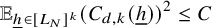 $$ \begin{align} {\mathbb E}_{{\underline{h}}\in [L_N]^k}(C_{d,k}({\underline{h}}))^2\leq C \end{align} $$
for every $N\in {\mathbb N}$
.
$N\in {\mathbb N}$
.
Note that since $L_N\succ (\log {N})^K$
for every
$L_N\succ (\log {N})^K$
for every $K>0$
and
$K>0$
and $\Lambda '(n)\leq \log {n}$
, for every
$\Lambda '(n)\leq \log {n}$
, for every $n\in {\mathbb N}$
, we have that
$n\in {\mathbb N}$
, we have that $\max _{{\underline {h}}\in [L_N]^k, n\in [N]}(\tilde {w}_{N,{\underline {h}}}(n))^2\prec L_N$
. Using this, and since by equation (11), we have that
$\max _{{\underline {h}}\in [L_N]^k, n\in [N]}(\tilde {w}_{N,{\underline {h}}}(n))^2\prec L_N$
. Using this, and since by equation (11), we have that $\frac {1}{L_N^k}|[L_N]^k\setminus ([L_N]^k)^*|\ll _k \frac {1}{L_N}$
, we deduce that we can redefine
$\frac {1}{L_N^k}|[L_N]^k\setminus ([L_N]^k)^*|\ll _k \frac {1}{L_N}$
, we deduce that we can redefine $C({\underline {h}})$
on the complement of
$C({\underline {h}})$
on the complement of $([L_N]^k)^*$
so that for all large enough N (depending on
$([L_N]^k)^*$
so that for all large enough N (depending on $d,k,p$
), equation (24) holds for all
$d,k,p$
), equation (24) holds for all $n\in I_{N,{\underline {h}}}$
,
$n\in I_{N,{\underline {h}}}$
, ${\underline {h}}\in [L_N]^k$
, and equation (25) also holds (for some larger constant
${\underline {h}}\in [L_N]^k$
, and equation (25) also holds (for some larger constant $C'$
in place of C).
$C'$
in place of C).
We now use equations (24) and (25) and the Cauchy-Schwarz inequality to bound the averages in equation (21). We can also remove the indicator $ \mathbf {1}_{I^{\prime }_{N,{\underline {h}}}}(n)$
since it has a negligible effect on our averages. We deduce that it suffices to get an upper bound for the averages
$ \mathbf {1}_{I^{\prime }_{N,{\underline {h}}}}(n)$
since it has a negligible effect on our averages. We deduce that it suffices to get an upper bound for the averages
 $$ \begin{align*} {\mathbb E}_{{\underline{h}}\in [L_N]^k} \left\Vert {\mathbb E}_{n\in I_{N,{\underline{h}}}}\, \, z_{N,{\underline{h}}}(n) \cdot \prod_{i=1}^\ell T^{[a_i({\underline{h}},(n/p({\underline{h}}))^{1/d})]+\epsilon_{i,N}} f_{N,{\underline{h}},i}\right\Vert^2_{L^2(\mu)}. \end{align*} $$
Note that since the weights and functions are bounded, it suffices to get an upper bound for the previous expression, ignoring the square. For ${\underline {h}}\in [L_N]^k$
, we can express
${\underline {h}}\in [L_N]^k$
, we can express $n\in I_{N,{\underline {h}}}$
as
$n\in I_{N,{\underline {h}}}$
as $n=n'p({\underline {h}})+s$
for some
$n=n'p({\underline {h}})+s$
for some $n'\in [N^{ad}]$
or
$n'\in [N^{ad}]$
or $n'=0$
and
$n'=0$
and $s\in [p({\underline {h}})]$
. After renaming
$s\in [p({\underline {h}})]$
. After renaming $n'$
as n for convenience, we are led to upper-bounding the averages
$n'$
as n for convenience, we are led to upper-bounding the averages
 $$ \begin{align} {\mathbb E}_{{\underline{h}}\in [L_N]^k}{\mathbb E}_{s\in [p({\underline{h}})]} \left\Vert {\mathbb E}_{n\in [N^{ad}]}\, \, z_{N,{\underline{h}},s}(n) \cdot \prod_{i=1}^\ell T^{[a_i({\underline{h}},(n+s/p({\underline{h}}))^{1/d})]+\epsilon_{i,N}} f_{N,{\underline{h}},i}\right\Vert_{L^2(\mu)} \end{align} $$
for some $1$
-bounded sequence
$1$
-bounded sequence $(z_{N,{\underline {h}},s}(n))$
. Note that if
$(z_{N,{\underline {h}},s}(n))$
. Note that if $u\in (0,1)$
and
$u\in (0,1)$
and $q\in {\mathbb R}[t_1,\ldots , t_k]$
, then an application of the mean value theorem shows that for every
$q\in {\mathbb R}[t_1,\ldots , t_k]$
, then an application of the mean value theorem shows that for every $\varepsilon>0$
, we have
$\varepsilon>0$
, we have
 $$ \begin{align*} \lim_{N\to\infty} \sup_{c\in [0,1], {\underline{h}}\in[L_N]^k,n\geq N^{\varepsilon}} | q({\underline{h}}) ((n+c)^u-n^u) | = 0. \end{align*} $$
It follows that in equation (26), when computing $a_i({\underline {h}},(n+s/p({\underline {h}}))^{1/d})$
, we can replace
$a_i({\underline {h}},(n+s/p({\underline {h}}))^{1/d})$
, we can replace $n+s/p({\underline {h}})$
with n in the nonlinear monomials; this will lead to some error sequences that are
$n+s/p({\underline {h}})$
with n in the nonlinear monomials; this will lead to some error sequences that are $1$
-bounded for large enough N and can be handled by appealing to Lemma 3.6 (and redefining the sequence
$1$
-bounded for large enough N and can be handled by appealing to Lemma 3.6 (and redefining the sequence $z_{N,{\underline {h}}}(n)$
). With this in mind, it follows that in equation (26), we can replace
$z_{N,{\underline {h}}}(n)$
). With this in mind, it follows that in equation (26), we can replace $a_i({\underline {h}},(n+s/p({\underline {h}}))^{1/d})$
with
$a_i({\underline {h}},(n+s/p({\underline {h}}))^{1/d})$
with $a_i({\underline {h}},n^{1/d})+\frac {p_{i,r}({\underline {h}})}{p({\underline {h}})}s$
. Hence, it suffices to get an upper bound for the averages
$a_i({\underline {h}},n^{1/d})+\frac {p_{i,r}({\underline {h}})}{p({\underline {h}})}s$
. Hence, it suffices to get an upper bound for the averages
 $$ \begin{align*} {\mathbb E}_{{\underline{h}}\in [L_N]^k}{\mathbb E}_{s\in [p({\underline{h}})]} \left\Vert {\mathbb E}_{n\in [N^{ad}]}\, \, z_{N,{\underline{h}}}(n) \cdot \prod_{i=1}^\ell T^{[a_i({\underline{h}},n^{1/d})+e_{i,N}({\underline{h}},s)]} f_{N,{\underline{h}},i}\right\Vert_{L^2(\mu)}, \end{align*} $$
where $e_{i,N}({\underline {h}},s):=\frac {p_{i,r}({\underline {h}})}{p({\underline {h}})}s+\epsilon _{i,N}$
,
$e_{i,N}({\underline {h}},s):=\frac {p_{i,r}({\underline {h}})}{p({\underline {h}})}s+\epsilon _{i,N}$
, $i=1,\ldots , \ell $
and
$i=1,\ldots , \ell $
and $\epsilon _{1,N},\ldots , \epsilon _{\ell ,N}$
take finitely many values for
$\epsilon _{1,N},\ldots , \epsilon _{\ell ,N}$
take finitely many values for $N\in {\mathbb N}$
. After replacing the average
$N\in {\mathbb N}$
. After replacing the average ${\mathbb E}_{s\in [p({\underline {h}})]}$
with
${\mathbb E}_{s\in [p({\underline {h}})]}$
with $\max _{s\in [p({\underline {h}})]}$
, we are led to the asserted upper bound in equation (18).
$\max _{s\in [p({\underline {h}})]}$
, we are led to the asserted upper bound in equation (18).
4.3 Reduction to averages with polynomial iterates
For the purposes of the next lemma, it will be convenient to slightly enlarge the class of polynomials with real exponents that we work with to include those with fractional degree equal to $1$
.
$1$
.
Lemma 4.2. Let $k\in {\mathbb Z}_+, \ell \in {\mathbb N}$
and
$k\in {\mathbb Z}_+, \ell \in {\mathbb N}$
and $a_1,\ldots , a_\ell \colon {\mathbb N}^k\times {\mathbb N}\to {\mathbb R}$
be a nice collection of polynomials with real exponents and k-parameters of fractional degree at most
$a_1,\ldots , a_\ell \colon {\mathbb N}^k\times {\mathbb N}\to {\mathbb R}$
be a nice collection of polynomials with real exponents and k-parameters of fractional degree at most $1$
. Then there exist
$1$
. Then there exist $l,r\in {\mathbb N}$
and nonconstant polynomials
$l,r\in {\mathbb N}$
and nonconstant polynomials $P_1,\ldots , P_r\in {\mathbb R}[t_1,\ldots , t_{k+l}]$
, with pairwise nonconstant differences, such that the following holds: If
$P_1,\ldots , P_r\in {\mathbb R}[t_1,\ldots , t_{k+l}]$
, with pairwise nonconstant differences, such that the following holds: If $(X,\mu ,T)$
is a system and
$(X,\mu ,T)$
is a system and $f_{N,{\underline {h}},1},\ldots , f_{N,{\underline {h}},\ell }\in L^\infty (\mu )$
,
$f_{N,{\underline {h}},1},\ldots , f_{N,{\underline {h}},\ell }\in L^\infty (\mu )$
, ${\underline {h}}\in {\mathbb N}^k,N\in {\mathbb N}$
, are
${\underline {h}}\in {\mathbb N}^k,N\in {\mathbb N}$
, are $1$
-bounded functions, then for every
$1$
-bounded functions, then for every $a>0$
, sequences of real numbers
$a>0$
, sequences of real numbers $(e_{1,N}({\underline {h}})),\ldots , (e_{\ell ,N}({\underline {h}}))$
and
$(e_{1,N}({\underline {h}})),\ldots , (e_{\ell ,N}({\underline {h}}))$
and $1$
-bounded sequence of complex numbers
$1$
-bounded sequence of complex numbers $(c_{N,{\underline {h}}}(n))$
, we have
$(c_{N,{\underline {h}}}(n))$
, we have
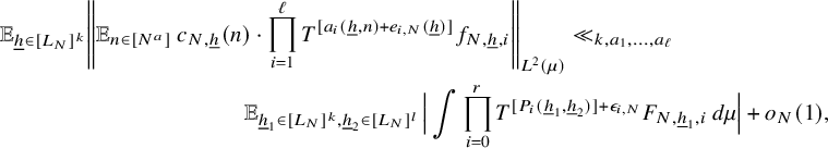 $$ \begin{align} {\mathbb E}_{{\underline{h}}\in [L_N]^k} &\left\Vert {\mathbb E}_{n\in [N^a]}\, c_{N,{\underline{h}}}(n) \cdot \prod_{i=1}^\ell T^{[a_i({\underline{h}},n)+e_{i,N}({\underline{h}})]} f_{N,{\underline{h}},i}\right\Vert_{L^2(\mu)}\ll_{k, a_1,\ldots, a_\ell} \nonumber\\ &\qquad\qquad\qquad\quad {\mathbb E}_{{\underline{h}}_1\in [L_N]^k,{\underline{h}}_2\in [L_N]^l} \,\Big| \int \prod_{i=0}^{r} T^{[P_i({\underline{h}}_1,{\underline{h}}_2)]+\epsilon_{i,N}} F_{N,{\underline{h}}_1, i} \, d\mu\Big| +o_N(1), \end{align} $$
where $P_0:=0$
,
$P_0:=0$
, $ F_{N,{\underline {h}}_1, i} \in \{f_{N,{\underline {h}}_1,1}, \overline {f}_{N,{\underline {h}}_1,1} \}$
for
$ F_{N,{\underline {h}}_1, i} \in \{f_{N,{\underline {h}}_1,1}, \overline {f}_{N,{\underline {h}}_1,1} \}$
for $i=0,\ldots , r$
,
$i=0,\ldots , r$
, ${\underline {h}}_1\in [L_N]^k,N\in {\mathbb N}$
,
${\underline {h}}_1\in [L_N]^k,N\in {\mathbb N}$
, $\epsilon _{0,N},\ldots , \epsilon _{r,N}$
take finitely many values for
$\epsilon _{0,N},\ldots , \epsilon _{r,N}$
take finitely many values for $N\in {\mathbb N}$
, and
$N\in {\mathbb N}$
, and $o_N(1)$
is a quantity that converges to
$o_N(1)$
is a quantity that converges to $0$
when
$0$
when $N\to \infty $
and all other parameters remain fixed.
$N\to \infty $
and all other parameters remain fixed.
Proof. We first reduce to the case where $e_{i,N}({\underline {h}})=0$
for
$e_{i,N}({\underline {h}})=0$
for $i=1, \ldots , \ell $
. To do this, we replace
$i=1, \ldots , \ell $
. To do this, we replace $[a_i({\underline {h}},n)+e_{i,N}({\underline {h}})]$
with
$[a_i({\underline {h}},n)+e_{i,N}({\underline {h}})]$
with $[a_i({\underline {h}},n)]+[e_{i,N}({\underline {h}})]$
; this introduces some error sequences on the exponents that take finitely many values. To treat the error sequences, we use Lemma 3.6, redefine the weight
$[a_i({\underline {h}},n)]+[e_{i,N}({\underline {h}})]$
; this introduces some error sequences on the exponents that take finitely many values. To treat the error sequences, we use Lemma 3.6, redefine the weight $(c_{N,{\underline {h}}}(n))$
and introduce some sequences
$(c_{N,{\underline {h}}}(n))$
and introduce some sequences $\epsilon _{1,N}, \ldots , \epsilon _{\ell ,N}$
that take finitely many values for
$\epsilon _{1,N}, \ldots , \epsilon _{\ell ,N}$
that take finitely many values for $N\in {\mathbb N}$
. Next, we compose with
$N\in {\mathbb N}$
. Next, we compose with $T^{-[e_{1,N}({\underline {h}})]-\epsilon _{1,N}}$
, and we are left with upper-bounding the expression
$T^{-[e_{1,N}({\underline {h}})]-\epsilon _{1,N}}$
, and we are left with upper-bounding the expression
 $$ \begin{align*} {\mathbb E}_{{\underline{h}}\in [L_N]^k} \left\Vert {\mathbb E}_{n\in [N^a]}\, c_{N,{\underline{h}}}(n) \cdot \prod_{i=1}^\ell T^{[a_i({\underline{h}},n)]} (T^{[e_{i,N}({\underline{h}})]-[e_{1,N}({\underline{h}})]+\epsilon_{i,N}-\epsilon_{1,N}}f_{N,{\underline{h}},i})\right\Vert_{L^2(\mu)}. \end{align*} $$
If we rename for $i=2,\ldots , \ell $
the functions
$i=2,\ldots , \ell $
the functions $T^{[e_{i,N}({\underline {h}})]-[e_{1,N}({\underline {h}})]+\epsilon _{i,N}-\epsilon _{1,N}}f_{N,{\underline {h}},i}$
as
$T^{[e_{i,N}({\underline {h}})]-[e_{1,N}({\underline {h}})]+\epsilon _{i,N}-\epsilon _{1,N}}f_{N,{\underline {h}},i}$
as $f_{N,{\underline {h}},i}$
, we are reduced to bounding equation (27) when
$f_{N,{\underline {h}},i}$
, we are reduced to bounding equation (27) when $e_{i,N}({\underline {h}})=0$
for
$e_{i,N}({\underline {h}})=0$
for $i=1, \ldots , \ell $
.
$i=1, \ldots , \ell $
.
We will prove the statement by induction on $\ell \in {\mathbb N}$
. For
$\ell \in {\mathbb N}$
. For $\ell =1$
, the argument is similar to the one used in the inductive step, so we only summarise it briefly (for more details; see Steps 1–3 below). We first use Lemma 4.1, and we are led to upper-bounding the averages
$\ell =1$
, the argument is similar to the one used in the inductive step, so we only summarise it briefly (for more details; see Steps 1–3 below). We first use Lemma 4.1, and we are led to upper-bounding the averages
 $$ \begin{align*} {\mathbb E}_{{\underline{h}}\in [L_N]^k} \left\Vert {\mathbb E}_{n\in [N^a]}\, c_{N,{\underline{h}}}(n) \cdot T^{[p_1({\underline{h}})n+q_1({\underline{h}},n)]} f_{N,{\underline{h}},1}\right\Vert_{L^2(\mu)}, \end{align*} $$
where $p_1\neq 0$
and
$p_1\neq 0$
and $q_1$
is a polynomial with real exponents and
$q_1$
is a polynomial with real exponents and $\text {f-deg}(q_1)<1$
. We then apply equation (15) for the average over n, compose with
$\text {f-deg}(q_1)<1$
. We then apply equation (15) for the average over n, compose with $T^{-[p_1({\underline {h}})n+q_1({\underline {h}},n)]}$
, use that
$T^{-[p_1({\underline {h}})n+q_1({\underline {h}},n)]}$
, use that $q_1({\underline {h}},n+h_{k+1})-q_1({\underline {h}},n)$
is negligible for the range of parameters we are interested in and use Lemma 3.6 to treat the finite valued error sequences that arise. We get an upper bound by the averages
$q_1({\underline {h}},n+h_{k+1})-q_1({\underline {h}},n)$
is negligible for the range of parameters we are interested in and use Lemma 3.6 to treat the finite valued error sequences that arise. We get an upper bound by the averages
 $$ \begin{align*} {\mathbb E}_{{\underline{h}}\in [L_N]^k, h_{k+1}\in [L_N]} \Big| \int T^{[p_1({\underline{h}})h_{k+1}]+\epsilon_N} f_{N,{\underline{h}},1} \cdot \overline{f}_{N,{\underline{h}},1} \, d\mu\Big|, \end{align*} $$
where $\epsilon _N$
takes finitely many values for
$\epsilon _N$
takes finitely many values for $N\in {\mathbb N}$
. This proves equation (27) (with
$N\in {\mathbb N}$
. This proves equation (27) (with $\ell =r=1$
).
$\ell =r=1$
).
Suppose that $\ell \geq 2$
and the statement holds for all nice collections of
$\ell \geq 2$
and the statement holds for all nice collections of $\ell -1$
polynomials with real exponents and finitely many parameters.
$\ell -1$
polynomials with real exponents and finitely many parameters.
We have that $a_i({\underline {h}},t):=\sum _{j=1}^r p_{i,j}({\underline {h}})t^{d_j}$
,
$a_i({\underline {h}},t):=\sum _{j=1}^r p_{i,j}({\underline {h}})t^{d_j}$
, $i=1,\ldots , \ell $
, where
$i=1,\ldots , \ell $
, where $0\leq d_1<\cdots <d_r=d\leq 1$
and
$0\leq d_1<\cdots <d_r=d\leq 1$
and $p_{i,j}\in {\mathbb R}[t_1,\ldots , t_k]$
. Furthermore, we can assume that the polynomial
$p_{i,j}\in {\mathbb R}[t_1,\ldots , t_k]$
. Furthermore, we can assume that the polynomial $p_{1,r}$
is nonzero, and hence the fractional degree of
$p_{1,r}$
is nonzero, and hence the fractional degree of $a_1$
is d.
$a_1$
is d.
Step 1 (Linearising the highest-order term). If the fractional degree of $a_1$
is
$a_1$
is $1$
, then we proceed to Step 2. If not, then Lemma 4.1 (for
$1$
, then we proceed to Step 2. If not, then Lemma 4.1 (for $w_{N,{\underline {h}}}:=c_{N,{\underline {h}}}$
) applies, and we get an estimate of the form equation (18). Hence, to get an estimate of the form equation (27), it suffices to get a similar estimate for the averages
$w_{N,{\underline {h}}}:=c_{N,{\underline {h}}}$
) applies, and we get an estimate of the form equation (18). Hence, to get an estimate of the form equation (27), it suffices to get a similar estimate for the averages
 $$ \begin{align*} {\mathbb E}_{{\underline{h}}\in [L_N]^k} \left\Vert {\mathbb E}_{n\in [N^{ad}]}\, c_{N,{\underline{h}}}(n) \cdot \prod_{i=1}^{\ell} T^{[\tilde{a}_i({\underline{h}},n)]+e_{i,N}({\underline{h}})} f_{N,{\underline{h}},i}\right\Vert_{L^2(\mu)}, \end{align*} $$
where $(c_{N,{\underline {h}}}(n))$
is another
$(c_{N,{\underline {h}}}(n))$
is another $1$
-bounded sequence,
$1$
-bounded sequence, $(e_{1,N}({\underline {h}})), \ldots , (e_{\ell ,N}({\underline {h}}))$
are sequences of real numbers and
$(e_{1,N}({\underline {h}})), \ldots , (e_{\ell ,N}({\underline {h}}))$
are sequences of real numbers and
 $$ \begin{align} \tilde{a}_i({\underline{h}},t):=p_{i,r}({\underline{h}})\,t+ q_i({\underline{h}},t), \quad \text{where} \quad q_i({\underline{h}},t):=\sum_{j=1}^{r-1} p_{i,j}({\underline{h}}) \, t^{\frac{d_j}{d}}, \quad i=1,\ldots, \ell. \end{align} $$
After composing with $T^{-e_{1,N}({\underline {h}})}$
and redefining the functions
$T^{-e_{1,N}({\underline {h}})}$
and redefining the functions $f_{N,{\underline {h}},i}$
,
$f_{N,{\underline {h}},i}$
, $i=2,\ldots , \ell $
, we are reduced to the case where
$i=2,\ldots , \ell $
, we are reduced to the case where $e_{i,N}({\underline {h}})=0$
for
$e_{i,N}({\underline {h}})=0$
for $i=1,\ldots , \ell $
. So we only treat this case henceforth. We also remark that since the collection
$i=1,\ldots , \ell $
. So we only treat this case henceforth. We also remark that since the collection $a_1,\ldots , a_\ell $
is nice, and
$a_1,\ldots , a_\ell $
is nice, and $\tilde {a}_i({\underline {h}},t)=a_i({\underline {h}},t^{1/d})$
,
$\tilde {a}_i({\underline {h}},t)=a_i({\underline {h}},t^{1/d})$
, $i=1,\ldots , \ell $
, the collection
$i=1,\ldots , \ell $
, the collection $\tilde {a}_1,\ldots , \tilde {a}_\ell $
is also nice.
$\tilde {a}_1,\ldots , \tilde {a}_\ell $
is also nice.
Step 2 (Reduction of $\ell $
via vdC). Applying equation (15) for the average over n, we get that it suffices to obtain an upper bound for the following averages:
$\ell $
via vdC). Applying equation (15) for the average over n, we get that it suffices to obtain an upper bound for the following averages:
 $$ \begin{align*} {\mathbb E}_{({\underline{h}}, h_{k+1})\in [L_N]^{k+1}} {\mathbb E}_{n\in [N^{ad}]}\Big| \int \prod_{i=1}^\ell T^{[\tilde{a}_i({\underline{h}},n+h_{k+1})]} f_{N,{\underline{h}},i}\, \prod_{i=1}^\ell T^{[\tilde{a}_i({\underline{h}},n)]} \overline{f}_{N,{\underline{h}},i}\, \, d\mu\Big|. \end{align*} $$
We compose with $T^{-[\tilde {a}_1({\underline {h}},n)]}$
, and for
$T^{-[\tilde {a}_1({\underline {h}},n)]}$
, and for $i=1,\ldots , \ell $
, we replace the differences
$i=1,\ldots , \ell $
, we replace the differences $[\tilde {a}_i({\underline {h}},n+h_{k+1})]-[\tilde {a}_1({\underline {h}},n)]$
,
$[\tilde {a}_i({\underline {h}},n+h_{k+1})]-[\tilde {a}_1({\underline {h}},n)]$
, $[\tilde {a}_i({\underline {h}},n)]-[\tilde {a}_1({\underline {h}},n)]$
with
$[\tilde {a}_i({\underline {h}},n)]-[\tilde {a}_1({\underline {h}},n)]$
with $[\tilde {a}_i({\underline {h}},n+h_{k+1})-\tilde {a}_1({\underline {h}},n)]$
,
$[\tilde {a}_i({\underline {h}},n+h_{k+1})-\tilde {a}_1({\underline {h}},n)]$
, $[\tilde {a}_i({\underline {h}},n)-\tilde {a}_1({\underline {h}},n)]$
, respectively. To do so, we have to introduce some error sequences that take values on a finite subset of
$[\tilde {a}_i({\underline {h}},n)-\tilde {a}_1({\underline {h}},n)]$
, respectively. To do so, we have to introduce some error sequences that take values on a finite subset of ${\mathbb N}$
. We use Lemma 3.6 to treat the errors that arise, and we are left with upper-bounding averages of the form
${\mathbb N}$
. We use Lemma 3.6 to treat the errors that arise, and we are left with upper-bounding averages of the form
 $$ \begin{align*} {\mathbb E}_{({\underline{h}}, h_{k+1})\in [L_N]^{k+1}} {\mathbb E}_{n\in [N^{ad}]}\Big| \int \prod_{i=1}^\ell T^{[\tilde{a}_i({\underline{h}},n+h_{k+1})-\tilde{a}_1({\underline{h}},n)]+\epsilon_{i,N}} &f_{N,{\underline{h}},i}\cdot \\ &\prod_{i=1}^\ell T^{[\tilde{a}_i({\underline{h}},n)-\tilde{a}_1({\underline{h}},n)]+\epsilon^{\prime}_{i,N} } \overline{f}_{N,{\underline{h}},i}\, \, d\mu\Big|, \end{align*} $$
where $\epsilon _{i,N},\epsilon ^{\prime }_{i,N}$
,
$\epsilon _{i,N},\epsilon ^{\prime }_{i,N}$
, $i=1,\ldots , \ell $
take finitely many values for
$i=1,\ldots , \ell $
take finitely many values for $N\in {\mathbb N}$
. Note that the fractional degree of
$N\in {\mathbb N}$
. Note that the fractional degree of $q_1, \ldots , q_\ell $
is strictly smaller than
$q_1, \ldots , q_\ell $
is strictly smaller than $1$
. It follows from this and the mean value theorem that
$1$
. It follows from this and the mean value theorem that
 $$ \begin{align} \lim_{N\to\infty}\max_{({\underline{h}},h_k)\in [L_N]^{k+1}, i\in \{1,\ldots, \ell\}}|q_i({\underline{h}},t+h_{k+1})-q_i({\underline{h}},t)|=0. \end{align} $$
Using equations (28) and (29) and then Lemma 3.6, we get that it suffices to get an upper bound for the averages
 $$ \begin{align*} {\mathbb E}_{({\underline{h}},h_{k+1})\in [L_N]^{k+1}} {\mathbb E}_{n\in [N^{ad}]}\, c_{N,{\underline{h}},h_{k+1}}(n) \cdot \int (T^{[p_{1,r}({\underline{h}})h_{k+1}]+\epsilon_{1,N} } &f_{N,{\underline{h}},1}\cdot \overline{f}_{N,{\underline{h}},1})\cdot \\ &\quad \prod_{i=2}^\ell T^{[b_i({\underline{h}},n)]+\epsilon_{i,N} }\tilde{f}_{N,{\underline{h}},h_{k+1},i}\, d\mu, \end{align*} $$
where $\epsilon _{1,N},\ldots , \epsilon _{\ell ,N}$
take finitely many values for
$\epsilon _{1,N},\ldots , \epsilon _{\ell ,N}$
take finitely many values for $N\in {\mathbb N}$
,
$N\in {\mathbb N}$
,
 $$ \begin{align*} b_{i}({\underline{h}},t):=(p_{i,r}-p_{1,r})({\underline{h}})\, t+(q_{i}-q_1)({\underline{h}},t), \quad i=2,\ldots, \ell, \end{align*} $$ $\tilde {f}_{N,{\underline {h}},h_{k+1},i}\in L^\infty (\mu )$
,
$\tilde {f}_{N,{\underline {h}},h_{k+1},i}\in L^\infty (\mu )$
, $i=2,\ldots , \ell $
are
$i=2,\ldots , \ell $
are $1$
-bounded functions and
$1$
-bounded functions and $(c_{N,{\underline {h}},h_{k+1}}(n))$
is a
$(c_{N,{\underline {h}},h_{k+1}}(n))$
is a $1$
-bounded sequence. Without loss of generality, we can assume that
$1$
-bounded sequence. Without loss of generality, we can assume that $b_\ell $
has maximal fractional degree within the collection
$b_\ell $
has maximal fractional degree within the collection $b_2,\ldots , b_\ell $
(note that some of the polynomials
$b_2,\ldots , b_\ell $
(note that some of the polynomials $p_{i,r}-p_{1,r}$
may vanish). We compose with
$p_{i,r}-p_{1,r}$
may vanish). We compose with $T^{-[b_\ell ({\underline {h}},n)]}$
and apply Lemma 3.6 to treat finite-valued error sequences that we get when we replace differences of integer parts with the integer part of the corresponding differences. After using the Cauchy-Schwarz inequality, we deduce that it suffices to get an upper bound for the following averages:
$T^{-[b_\ell ({\underline {h}},n)]}$
and apply Lemma 3.6 to treat finite-valued error sequences that we get when we replace differences of integer parts with the integer part of the corresponding differences. After using the Cauchy-Schwarz inequality, we deduce that it suffices to get an upper bound for the following averages:
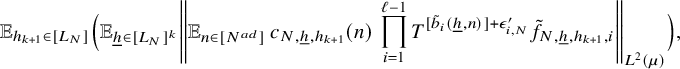 $$ \begin{align} {\mathbb E}_{h_{k+1}\in [L_N]} \Big({\mathbb E}_{{\underline{h}}\in [L_N]^k} \left\Vert {\mathbb E}_{n\in [N^{ad}]} \, c_{N,{\underline{h}},h_{k+1}}(n) \, \prod_{i=1}^{\ell-1} T^{[\tilde{b}_i({\underline{h}},n)]+\epsilon^{\prime}_{i,N}}\tilde{f}_{N,{\underline{h}},h_{k+1},i}\right\Vert_{L^2(\mu)}\Big), \end{align} $$
where $ \epsilon ^{\prime }_{1,N},\ldots , \epsilon ^{\prime }_{\ell -1,N}$
take finitely many values for
$ \epsilon ^{\prime }_{1,N},\ldots , \epsilon ^{\prime }_{\ell -1,N}$
take finitely many values for $N\in {\mathbb N}$
,
$N\in {\mathbb N}$
,
 $$ \begin{align*} \tilde{b}_{i}({\underline{h}},t):=(p_{i,r}-p_{\ell,r})({\underline{h}})\, t+(q_{i}-q_\ell)({\underline{h}},t), \quad i=1,\ldots, \ell-1, \end{align*} $$
and
 $$ \begin{align} \tilde{f}_{N,{\underline{h}},h_{k+1},1}:= T^{[p_{1,r}({\underline{h}})h_{k+1}]+\epsilon_{1,N}}f_{N,{\underline{h}}, 1}\cdot \overline{f}_{N,{\underline{h}}, 1}, \end{align} $$
where $ \epsilon _{1,N}$
takes finitely many values for
$ \epsilon _{1,N}$
takes finitely many values for $N\in {\mathbb N}$
.
$N\in {\mathbb N}$
.
Note that our assumptions imply that $\tilde {b}_{1},\ldots , \tilde {b}_{\ell -1}$
, thought of as a collection of polynomials with real exponents and
$\tilde {b}_{1},\ldots , \tilde {b}_{\ell -1}$
, thought of as a collection of polynomials with real exponents and $(k+1)$
-parameters, is nice.
$(k+1)$
-parameters, is nice.
Step 3 (Applying the induction hypothesis). Using the induction hypothesis for the expression in equation (30) that is inside the parentheses, and the fact that $\tilde {b}_1,\ldots , \tilde {b}_{\ell -1}$
do not depend on the parameter
$\tilde {b}_1,\ldots , \tilde {b}_{\ell -1}$
do not depend on the parameter $h_{k+1}$
, we get that there exist
$h_{k+1}$
, we get that there exist $l,r\in {\mathbb N}$
and nonconstant polynomials
$l,r\in {\mathbb N}$
and nonconstant polynomials $P_1,\ldots , P_r\in {\mathbb R}[t_1,\ldots , t_{k+l}]$
with pairwise nonconstant differences, such that the averages in equation (30) are bounded by an
$P_1,\ldots , P_r\in {\mathbb R}[t_1,\ldots , t_{k+l}]$
with pairwise nonconstant differences, such that the averages in equation (30) are bounded by an $o_N(1)$
term plus a constant
$o_N(1)$
term plus a constant $C_{k,a_1,\ldots , a_\ell }$
(note that
$C_{k,a_1,\ldots , a_\ell }$
(note that $\tilde {b}_{1},\ldots , \tilde {b}_{\ell -1}$
are determined by
$\tilde {b}_{1},\ldots , \tilde {b}_{\ell -1}$
are determined by $a_1,\ldots , a_\ell $
) times the expression
$a_1,\ldots , a_\ell $
) times the expression
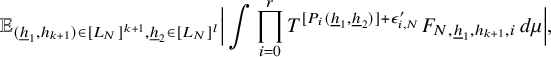 $$ \begin{align*} {\mathbb E}_{({\underline{h}}_1,h_{k+1})\in [L_N]^{k+1},{\underline{h}}_2\in [L_N]^l}\Big| \int \prod_{i=0}^{r} T^{[P_i({\underline{h}}_1,{\underline{h}}_2)]+\epsilon^{\prime}_{i,N}} F_{N,{\underline{h}}_1, h_{k+1},i}\, d\mu\Big|, \end{align*} $$
where $P_0:=0$
,
$P_0:=0$
, $ F_{N,{\underline {h}},h_{k+1},i} \in \{ \tilde {f}_{N,{\underline {h}},h_{k+1},1}, \overline {\tilde {f}}_{N,{\underline {h}},h_{k+1},1} \}$
for
$ F_{N,{\underline {h}},h_{k+1},i} \in \{ \tilde {f}_{N,{\underline {h}},h_{k+1},1}, \overline {\tilde {f}}_{N,{\underline {h}},h_{k+1},1} \}$
for $i=0,\ldots , r$
,
$i=0,\ldots , r$
, ${\underline {h}}_1\in [L_N]^k$
,
${\underline {h}}_1\in [L_N]^k$
, $h_{k+1}\in [L_N]$
,
$h_{k+1}\in [L_N]$
, $N\in {\mathbb N}$
and
$N\in {\mathbb N}$
and $\epsilon ^{\prime }_{0,N},\ldots , \epsilon ^{\prime }_{r,N}$
take finitely many values for
$\epsilon ^{\prime }_{0,N},\ldots , \epsilon ^{\prime }_{r,N}$
take finitely many values for $N\in {\mathbb N}$
.
$N\in {\mathbb N}$
.
Using equation (31) and Lemma 3.6, we can bound this expression by a constant $C_{r}$
times the following average:
$C_{r}$
times the following average:
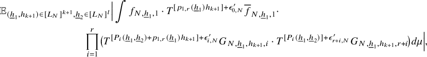 $$ \begin{align*} &{\mathbb E}_{({\underline{h}}_1,h_{k+1})\in [L_N]^{k+1},{\underline{h}}_2\in [L_N]^l} \Big|\int f_{N,{\underline{h}}_1, 1} \cdot T^{[p_{1,r}({\underline{h}}_1)h_{k+1}]+\epsilon^{\prime}_{0,N}}\overline{f}_{N,{\underline{h}}_1, 1}\cdot\\ &\qquad\qquad\qquad\qquad \prod_{i=1}^{r} \!\big(T^{[P_i({\underline{h}}_1,{\underline{h}}_2)+p_{1,r}({\underline{h}}_1)h_{k+1}]+\epsilon^{\prime}_{i,N}} G_{N,{\underline{h}}_1,h_{k+1},i}\cdot T^{[P_i({\underline{h}}_1,{\underline{h}}_2)]+\epsilon^{\prime}_{r+i,N}} G_{N,{\underline{h}}_1,h_{k+1},r+i}\!\big) d\mu\Big|, \end{align*} $$
where for $i=1,\ldots , 2r$
, we have
$i=1,\ldots , 2r$
, we have $G_{N,{\underline {h}}_1,h_{k+1},i} \in \{ f_{N,{\underline {h}}_1,1}, \overline {f}_{N,{\underline {h}}_1,1} \}$
,
$G_{N,{\underline {h}}_1,h_{k+1},i} \in \{ f_{N,{\underline {h}}_1,1}, \overline {f}_{N,{\underline {h}}_1,1} \}$
, ${\underline {h}}_1 \in [L_N]^k$
,
${\underline {h}}_1 \in [L_N]^k$
, $h_{k+1}\in [L_N]$
,
$h_{k+1}\in [L_N]$
, $N\in {\mathbb N}$
, and
$N\in {\mathbb N}$
, and $\epsilon ^{\prime }_{i,N}$
,
$\epsilon ^{\prime }_{i,N}$
, $i=0,\ldots , 2r$
take finitely many values for
$i=0,\ldots , 2r$
take finitely many values for $N\in {\mathbb N}$
. Since the polynomial
$N\in {\mathbb N}$
. Since the polynomial $p_{1,r}$
is nonzero and the polynomials
$p_{1,r}$
is nonzero and the polynomials $P_1,\ldots , P_r$
with
$P_1,\ldots , P_r$
with $k+l$
variables are nonconstant and have nonconstant pairwise differences, the same holds for the
$k+l$
variables are nonconstant and have nonconstant pairwise differences, the same holds for the $2r+1$
polynomials with
$2r+1$
polynomials with $k+l+1$
variables
$k+l+1$
variables $p_{1,r}({\underline {h}}_1)h_{k+1}$
,
$p_{1,r}({\underline {h}}_1)h_{k+1}$
, $P_i({\underline {h}}_1,{\underline {h}}_2)+p_{1,r}({\underline {h}}_1)h_{k+1}$
,
$P_i({\underline {h}}_1,{\underline {h}}_2)+p_{1,r}({\underline {h}}_1)h_{k+1}$
, $P_i({\underline {h}}_1,{\underline {h}}_2)$
,
$P_i({\underline {h}}_1,{\underline {h}}_2)$
, $i=1,\ldots , r$
. This completes the proof.
$i=1,\ldots , r$
. This completes the proof.
4.4 Averages with polynomial iterates
Lemma 4.1 and Lemma 4.2 show that in the case of iterates with sublinear growth, to get good seminorm estimates for the averages in Theorem 3.1, it suffices to study averages with iterates given by polynomials in ${\mathbb R}[t_1,\ldots , t_k]$
for some
${\mathbb R}[t_1,\ldots , t_k]$
for some $k\in {\mathbb N}$
. This is the context of the next result.
$k\in {\mathbb N}$
. This is the context of the next result.
Lemma 4.3. Let $k,r\in {\mathbb N}$
and
$k,r\in {\mathbb N}$
and $P_1,\ldots , P_r\in {\mathbb R}[t_1,\ldots , t_k]$
be nonconstant polynomials with pairwise nonconstant differences. Then there exists
$P_1,\ldots , P_r\in {\mathbb R}[t_1,\ldots , t_k]$
be nonconstant polynomials with pairwise nonconstant differences. Then there exists $s\in {\mathbb N}$
such that the following holds: If
$s\in {\mathbb N}$
such that the following holds: If $(X,\mu ,T)$
is an ergodic system and
$(X,\mu ,T)$
is an ergodic system and $f_1,\ldots , f_r\in L^\infty (\mu )$
are such that
$f_1,\ldots , f_r\in L^\infty (\mu )$
are such that $\lvert \!|\!| f_i|\!|\!\rvert _s=0$
for some
$\lvert \!|\!| f_i|\!|\!\rvert _s=0$
for some $i\in \{1,\ldots , r\}$
, then for every
$i\in \{1,\ldots , r\}$
, then for every $1$
-bounded sequence
$1$
-bounded sequence $(c_N({\underline {h}}))$
, we have
$(c_N({\underline {h}}))$
, we have
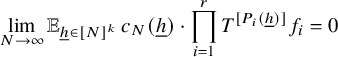 $$ \begin{align*} \lim_{N\to\infty} {\mathbb E}_{{\underline{h}}\in [N]^k}\, c_{N}({\underline{h}})\cdot \prod_{i=1}^{r} T^{[P_i({\underline{h}})]} f_i=0 \end{align*} $$
in $L^2(\mu )$
.
$L^2(\mu )$
.
Proof. The argument is similar to the one used to prove [Reference Leibman23, Theorem 1], where the case of polynomials with integer coefficients and $c_{N}({\underline {h}}):=1$
is covered, so we only sketch the points in the argument where one has to deviate slightly because of minor technical complications. The proof proceeds by induction on a certain vector, called the weight, that is associated to each polynomial family
$c_{N}({\underline {h}}):=1$
is covered, so we only sketch the points in the argument where one has to deviate slightly because of minor technical complications. The proof proceeds by induction on a certain vector, called the weight, that is associated to each polynomial family $P_1,\ldots , P_r$
in
$P_1,\ldots , P_r$
in ${\mathbb R}[t_1,\ldots , t_k]$
.
${\mathbb R}[t_1,\ldots , t_k]$
.
The inductive step is carried out by using a variant of Lemma 3.5 in the form used in equation (16) that concerns averages over $[N]^k$
(see [Reference Leibman23, Lemma 4] for the precise statement). The argument applies verbatim in our case; the only change is that we need at various instances to replace the differences of the integer part of polynomials with the integer part of their differences; we do this with the help of Lemma 3.6, and the use of the constants
$[N]^k$
(see [Reference Leibman23, Lemma 4] for the precise statement). The argument applies verbatim in our case; the only change is that we need at various instances to replace the differences of the integer part of polynomials with the integer part of their differences; we do this with the help of Lemma 3.6, and the use of the constants $(c_N({\underline {h}}))$
facilitates this task.
$(c_N({\underline {h}}))$
facilitates this task.
The base case of the induction is the case where all the polynomials are linear with respect to all variables involved. This case is covered using another induction, this time on the number r of linear functions. The inductive step is proved using [Reference Leibman23, Lemma 4]. The only difference in our case, versus the argument used in [Reference Leibman23, Proposition 5], appears in the proof of the estimate
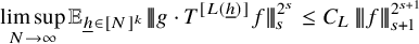 $$ \begin{align} \limsup_{N\to\infty}{\mathbb E}_{{\underline{h}}\in [N]^k}\lvert\!|\!| g\cdot T^{[L({\underline{h}})]}f|\!|\!\rvert^{2^s}_{s}\leq C_L\, \lvert\!|\!| f|\!|\!\rvert^{2^{s+1}}_{s+1} \end{align} $$
for some $C_{L}>0$
, where
$C_{L}>0$
, where $f,g\in L^\infty (\mu )$
and
$f,g\in L^\infty (\mu )$
and $L({\underline {h}})=\sum _{j=1}^k\alpha _j h_j$
for some
$L({\underline {h}})=\sum _{j=1}^k\alpha _j h_j$
for some $k\in {\mathbb N}$
and
$k\in {\mathbb N}$
and $\alpha _1,\ldots , \alpha _k\in {\mathbb R}$
. To obtain this bound, we first use Lemma 3.6 to show that it suffices to replace
$\alpha _1,\ldots , \alpha _k\in {\mathbb R}$
. To obtain this bound, we first use Lemma 3.6 to show that it suffices to replace $[\sum _{j=1}^k\alpha _j h_j]$
with
$[\sum _{j=1}^k\alpha _j h_j]$
with $\sum _{j=1}^k[\alpha _j h_j]$
, and we remark that the set
$\sum _{j=1}^k[\alpha _j h_j]$
, and we remark that the set
 $$ \begin{align*} \{([\alpha_1 h_1],\ldots, [\alpha_k h_k])\colon (h_1,\ldots, h_k)\in {\mathbb N}^k\} \end{align*} $$
has bounded multiplicity and positive density (as a subset of ${\mathbb N}^k$
). It follows that there exists
${\mathbb N}^k$
). It follows that there exists $C_L>0$
such that
$C_L>0$
such that
 $$ \begin{align*} \limsup_{N\to\infty}{\mathbb E}_{{\underline{h}}\in [N]^k}\lvert\!|\!| g\cdot T^{\sum_{j=1}^k[\alpha_j h_j]}f|\!|\!\rvert^{2^s}_{s}\leq C_L\, \limsup_{N\to\infty}{\mathbb E}_{{\underline{h}}\in [N]^k}\lvert\!|\!| g\cdot T^{\sum_{j=1}^k h_j}f|\!|\!\rvert^{2^s}_{s}. \end{align*} $$
By [Reference Leibman23, Lemma 8], the last expression is bounded by a constant multiple of $\lvert \!|\!| f|\!|\!\rvert ^{2^{s+1}}_{s+1}$
. Combining the above, we get that equation (32) holds. Finally, the base case of the induction (of the linear case) is when
$\lvert \!|\!| f|\!|\!\rvert ^{2^{s+1}}_{s+1}$
. Combining the above, we get that equation (32) holds. Finally, the base case of the induction (of the linear case) is when $r=1$
and
$r=1$
and $P_1=L$
is linear. To cover this case, we again use [Reference Leibman23, Lemma 4] and reduce matters to the task of obtaining an upper bound for the expression
$P_1=L$
is linear. To cover this case, we again use [Reference Leibman23, Lemma 4] and reduce matters to the task of obtaining an upper bound for the expression
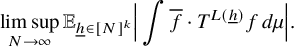 $$ \begin{align*} \limsup_{N\to\infty}{\mathbb E}_{{\underline{h}}\in [N]^k}\Big|\int \overline{f}\cdot T^{L({\underline{h}})}f\, d\mu\Big|. \end{align*} $$
By the $s=1$
case of equation (32) (recall that
$s=1$
case of equation (32) (recall that $\lvert \!|\!| f|\!|\!\rvert _1=|\int f\, d\mu |$
), we get an upper bound by
$\lvert \!|\!| f|\!|\!\rvert _1=|\int f\, d\mu |$
), we get an upper bound by $C_L\lvert \!|\!| f|\!|\!\rvert _2^2$
for some
$C_L\lvert \!|\!| f|\!|\!\rvert _2^2$
for some $C_L>0$
. This completes the proof.
$C_L>0$
. This completes the proof.
4.5 Proof of Theorem 3.1 in the sublinear case
We are now ready to combine the ingredients of the previous subsections to complete the goal of this section, which is to prove the following result:
Proposition 4.4. Theorem 3.1 holds in the case where all $a_1,\ldots , a_\ell $
have fractional degree smaller than one.
$a_1,\ldots , a_\ell $
have fractional degree smaller than one.
Proof. Combining Lemma 4.1 and Lemma 4.2 (for $f_{N,{\underline {h}},1}:=f_1$
,
$f_{N,{\underline {h}},1}:=f_1$
, $N\in {\mathbb N}, {\underline {h}}\in {\mathbb N}^k$
), we get that there exist
$N\in {\mathbb N}, {\underline {h}}\in {\mathbb N}^k$
), we get that there exist $k,r\in {\mathbb N}$
and nonconstant polynomials
$k,r\in {\mathbb N}$
and nonconstant polynomials $P_1,\ldots , P_r\in {\mathbb R}[t_1,\ldots , t_{k}]$
, with pairwise nonconstant differences, such that the averages in equation (8) are bounded by an
$P_1,\ldots , P_r\in {\mathbb R}[t_1,\ldots , t_{k}]$
, with pairwise nonconstant differences, such that the averages in equation (8) are bounded by an $o_N(1)$
term plus a constant multiple of
$o_N(1)$
term plus a constant multiple of
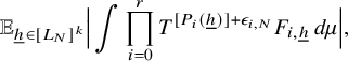 $$ \begin{align*} {\mathbb E}_{{\underline{h}}\in [L_N]^{k}}\Big|\int \prod_{i=0}^{r} T^{[P_i({\underline{h}})]+ \epsilon_{i,N}} F_{i,{\underline{h}}}\, d\mu\Big|, \end{align*} $$
where $P_0:=0$
,
$P_0:=0$
, $F_{0,{\underline {h}}},\ldots , F_{r,{\underline {h}}}\in \{f_1,\overline {f}_1\}$
,
$F_{0,{\underline {h}}},\ldots , F_{r,{\underline {h}}}\in \{f_1,\overline {f}_1\}$
, ${\underline {h}}\in {\mathbb N}^k$
and the sequences
${\underline {h}}\in {\mathbb N}^k$
and the sequences $\epsilon _{0,N},\ldots , \epsilon _{r,N}$
take values on a finite subset S of
$\epsilon _{0,N},\ldots , \epsilon _{r,N}$
take values on a finite subset S of ${\mathbb Z}$
for
${\mathbb Z}$
for $N\in {\mathbb N}$
. Since the limsup as
$N\in {\mathbb N}$
. Since the limsup as $N\to \infty $
of the previous average is bounded by
$N\to \infty $
of the previous average is bounded by
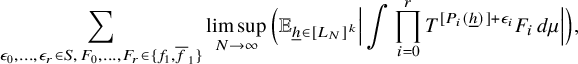 $$ \begin{align*} \sum_{\epsilon_0,\ldots, \epsilon_r\in S,\, F_0,\ldots, F_r\in \{f_1,\overline{f}_1\}}\limsup_{N\to\infty}\Big({\mathbb E}_{{\underline{h}}\in [L_N]^{k}}\Big|\int \prod_{i=0}^{r} T^{[P_i({\underline{h}})]+ \epsilon_{i}} F_{ i}\, d\mu\Big|\Big), \end{align*} $$
it suffices to show that for all fixed $\epsilon _0,\ldots , \epsilon _r\in {\mathbb Z}$
and
$\epsilon _0,\ldots , \epsilon _r\in {\mathbb Z}$
and $F_{0},\ldots , F_{r}\in \{f_1,\overline {f}_1\}$
, we have
$F_{0},\ldots , F_{r}\in \{f_1,\overline {f}_1\}$
, we have
 $$ \begin{align*} \lim_{N\to\infty}{\mathbb E}_{{\underline{h}}\in [L_N]^{k}}\Big|\int \prod_{i=0}^{r} T^{[P_i({\underline{h}})]+ \epsilon_{i}} F_{ i}\, d\mu\Big|=0. \end{align*} $$
The last average is equal to
 $$ \begin{align*} {\mathbb E}_{{\underline{h}}\in [L_N]^{k}}\, c_N({\underline{h}})\cdot \int \prod_{i=0}^{r} T^{[P_i({\underline{h}})+\epsilon_i]} F_{ i}\, d\mu \end{align*} $$
for some $1$
-bounded sequence
$1$
-bounded sequence $(c_N({\underline {h}}))$
. The result now follows from Lemma 4.3.
$(c_N({\underline {h}}))$
. The result now follows from Lemma 4.3.
5 Seminorm estimates – induction step
The goal of this section is to finish the proof of Theorem 3.1 using a PET-induction argument. The basis of the induction was covered in the previous section, and the induction step will be carried out in this section.
5.1 An example
To better illustrate our method, we first explain the details in a simple case. We take $\ell =2$
and
$\ell =2$
and $a_1(t):=t^{1.5}, a_2(t)=t^{1.5}+ t^{1.1}$
,
$a_1(t):=t^{1.5}, a_2(t)=t^{1.5}+ t^{1.1}$
, $t\in {\mathbb R}_+$
. Then
$t\in {\mathbb R}_+$
. Then $\{a_1,a_2\}$
is a nice family, and our aim is to show that if
$\{a_1,a_2\}$
is a nice family, and our aim is to show that if $\lvert \!|\!| f_1|\!|\!\rvert _s=0$
for some
$\lvert \!|\!| f_1|\!|\!\rvert _s=0$
for some $s\in {\mathbb N}$
, then
$s\in {\mathbb N}$
, then
 $$ \begin{align*}\lim_{N\to\infty} {\mathbb E}_{n\in [N]}\, w_N(n) \cdot T^{[n^{1.5}]}f_1\cdot T^{[n^{1.5}+n^{1.1}]}f_2=0, \end{align*} $$
where $w_N(n)=\Lambda '(n)\cdot c_N(n)$
for some
$w_N(n)=\Lambda '(n)\cdot c_N(n)$
for some $1$
-bounded sequence
$1$
-bounded sequence $(c_N(n))$
.
$(c_N(n))$
.
We start by using equation (15), compose with $T^{-[n^{1.5}+n^{1.1}]}$
, use Lemma 3.6 to dispose the error sequence that arises when we replace the difference of integer parts with the integer part of the difference and use the Cauchy-Schwarz inequality. We deduce that it suffices to prove convergence to zero of the averages
$T^{-[n^{1.5}+n^{1.1}]}$
, use Lemma 3.6 to dispose the error sequence that arises when we replace the difference of integer parts with the integer part of the difference and use the Cauchy-Schwarz inequality. We deduce that it suffices to prove convergence to zero of the averages
 $$ \begin{align*} {\mathbb E}_{h_1\in [L_N]}\Big|\Big|{\mathbb E}_{n\in [N]} \, w_{N,h_1}(n) \cdot T^{[(n+h_1)^{1.5}-n^{1.5}-n^{1.1}]} &f_1\cdot \\ & T^{[(n+h_1)^{1.5}+(n+h_1)^{1.1}-n^{1.5}-n^{1.1}]}f_2 \cdot T^{[-n^{1.1}]}\overline{f}_1\Big|\Big|_{L^2(\mu)}, \end{align*} $$
where $w_{N,h_1}(n):= (\Delta _{h_1}\Lambda ')(n)\cdot c_{N,h_1}(n)$
for some
$w_{N,h_1}(n):= (\Delta _{h_1}\Lambda ')(n)\cdot c_{N,h_1}(n)$
for some $1$
-bounded sequence
$1$
-bounded sequence $(c_{N,h_1}(n))$
. Using the mean value theorem and Lemma 3.6, we get that for the range of
$(c_{N,h_1}(n))$
. Using the mean value theorem and Lemma 3.6, we get that for the range of $h_1,n$
we are working with, we can replace
$h_1,n$
we are working with, we can replace $(n+h_1)^{1.5}-n^{1.5}$
with
$(n+h_1)^{1.5}-n^{1.5}$
with $1.5\, h_1n^{0.5}$
and
$1.5\, h_1n^{0.5}$
and $(n+h_1)^{1.1}-n^{1.1}$
with
$(n+h_1)^{1.1}-n^{1.1}$
with $1.1\, h_1n^{0.1}$
, which for notational simplicity we replace with
$1.1\, h_1n^{0.1}$
, which for notational simplicity we replace with $h_1n^{0.5}$
and
$h_1n^{0.5}$
and $h_1n^{0.1}$
, respectively. We thus arrive at the problem of proving convergence to zero of the averages
$h_1n^{0.1}$
, respectively. We thus arrive at the problem of proving convergence to zero of the averages
 $$ \begin{align*}{\mathbb E}_{h_1\in [L_N]}\left\Vert {\mathbb E}_{n\in [N]} \, w_{N,h_1}(n)\cdot T^{[-n^{1.1}+h_1n^{0.5}]}f_1\cdot T^{[h_1n^{0.5}+h_1 n^{0.1}]}f_2 \cdot T^{[-n^{1.1}]}\overline{f}_1\right\Vert_{L^2(\mu)}. \end{align*} $$
Performing one more time the previous operation (we compose with $T^{-[h_1n^{0.5}+h_1 n^{0.1}]}$
after applying equation (15)), we arrive in a similar fashion at the following averages:
$T^{-[h_1n^{0.5}+h_1 n^{0.1}]}$
after applying equation (15)), we arrive in a similar fashion at the following averages:
 $$ \begin{align*} {\mathbb E}_{h_1,h_2\in [L_N]}\Big|\Big|{\mathbb E}_{n\in [N]} \,w_{N,h_1,h_2}(n) \cdot T^{[-n^{1.1}-h_2 n^{0.1}]}f_1 &\cdot T^{[-n^{1.1}-h_1n^{0.5}-(h_1+h_2) n^{0.1}]}\overline{f}_1\cdot \\ & T^{[-n^{1.1}-h_1 n^{0.1}]}\overline{f}_1 \cdot T^{[-n^{1.1}-h_1n^{0.5}-h_1 n^{0.1}]}f_1\Big|\Big|_{L^2(\mu)}, \end{align*} $$
where $w_{N,h_1,h_2}(n):= (\Delta _{h_1,h_2}\Lambda ')(n)\cdot c_{N,h_1,h_2}(n)$
for some
$w_{N,h_1,h_2}(n):= (\Delta _{h_1,h_2}\Lambda ')(n)\cdot c_{N,h_1,h_2}(n)$
for some $1$
-bounded sequence
$1$
-bounded sequence $(c_{N,h_1,h_2}(n))$
. After one more iteration of the previous operation (this time we compose with the transformation
$(c_{N,h_1,h_2}(n))$
. After one more iteration of the previous operation (this time we compose with the transformation $T^{[n^{1.1}+h_1n^{0.5}+h_1 n^{0.1}]}$
after applying equation (15)), we arrive at the averages
$T^{[n^{1.1}+h_1n^{0.5}+h_1 n^{0.1}]}$
after applying equation (15)), we arrive at the averages
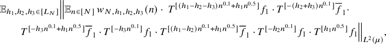 $$ \begin{align*} &{\mathbb E}_{h_1,h_2,h_3\in [L_N]} \Big|\Big| {\mathbb E}_{n\in [N]}\, w_{N,h_1,h_2,h_3}(n) \cdot \ T^{[(h_1-h_2-h_3) n^{0.1}+h_1n^{0.5}]}f_1 \cdot T^{[-(h_2+h_3) n^{0.1}]}\overline{f}_1\cdot \\ &\qquad T^{[-h_3 n^{0.1}+h_1n^{0.5}]}\overline{f}_1 \cdot T^{[-h_3 n^{0.1}]}f_1\cdot T^{[(h_1-h_2) n^{0.1}+h_1n^{0.5}]}\overline{f}_1 \cdot T^{[-h_2 n^{0.1}]}f_1\cdot T^{[h_1n^{0.5}]}f_1 \Big|\Big|_{L^2(\mu)}, \end{align*} $$
where $w_{N,h_1,h_2,h_3}(n):= (\Delta _{h_1,h_2,h_3}\Lambda ')(n)\cdot c_{N,h_1,h_2,h_3}(n)$
for some
$w_{N,h_1,h_2,h_3}(n):= (\Delta _{h_1,h_2,h_3}\Lambda ')(n)\cdot c_{N,h_1,h_2,h_3}(n)$
for some $1$
-bounded sequence
$1$
-bounded sequence $(c_{N,h_1,h_2,h_3}(n))$
. We have now reduced to the case of fractional polynomials with
$(c_{N,h_1,h_2,h_3}(n))$
. We have now reduced to the case of fractional polynomials with $3$
-parameters and fractional degree smaller than
$3$
-parameters and fractional degree smaller than $1$
. This case was dealt in the previous section, where we showed in Proposition 4.4 that there exists
$1$
. This case was dealt in the previous section, where we showed in Proposition 4.4 that there exists $s\in {\mathbb N}$
such that if
$s\in {\mathbb N}$
such that if $\lvert \!|\!| f_1|\!|\!\rvert _s=0$
, then the last averages converge to zero as
$\lvert \!|\!| f_1|\!|\!\rvert _s=0$
, then the last averages converge to zero as $N\to \infty $
.
$N\to \infty $
.
5.2 The van der Corput operation and reduction of type
In this subsection, we define the type of a family of polynomials with real exponents and finitely many parameters and the van der Corput operation that reduces the type.
Definition. We say that two polynomials $a, b$
with real exponents and finitely many parameters are equivalent, and write
$a, b$
with real exponents and finitely many parameters are equivalent, and write $a\cong b$
, if the (integral) degree of
$a\cong b$
, if the (integral) degree of $a- b$
is strictly smaller than the degree of a and b.Footnote
9
$a- b$
is strictly smaller than the degree of a and b.Footnote
9
We define the type of a family $a_1,\ldots , a_\ell $
of polynomials with real exponents and finitely many parameters to be the vector that consists of the maximal degree d of the family (in the first coordinate) and the number of nonequivalent classes of degree d,
$a_1,\ldots , a_\ell $
of polynomials with real exponents and finitely many parameters to be the vector that consists of the maximal degree d of the family (in the first coordinate) and the number of nonequivalent classes of degree d, $d-1$
,
$d-1$
, $\ldots $
,
$\ldots $
, $0$
in the other coordinates (we ignore polynomials that are identically
$0$
in the other coordinates (we ignore polynomials that are identically $0$
).
$0$
).
We order the set of all possible types lexicographically, meaning $(d, k_d,\ldots , k_0)>(d', k_d',\ldots , k_0')$
if and only if in the first instance where the two vectors disagree, the coordinate of the first vector is larger than the coordinate of the second vector.
$(d, k_d,\ldots , k_0)>(d', k_d',\ldots , k_0')$
if and only if in the first instance where the two vectors disagree, the coordinate of the first vector is larger than the coordinate of the second vector.
We caution the reader that $t^{2.5}\not \cong t^{2.5}+t^{2.1}$
(but
$t^{2.5}\not \cong t^{2.5}+t^{2.1}$
(but $t^{2.5}\cong t^{2.5}+t^{1.1}$
). Also, if
$t^{2.5}\cong t^{2.5}+t^{1.1}$
). Also, if $a_1(h,t)=ht^{2.5}+h^2t^{2.1}$
,
$a_1(h,t)=ht^{2.5}+h^2t^{2.1}$
, $a_2(h,t)=ht^{2.5}$
,
$a_2(h,t)=ht^{2.5}$
, $a_3(h,t)=ht^{2.5}+h^2t^{2.1}+ht^{1.5}$
,
$a_3(h,t)=ht^{2.5}+h^2t^{2.1}+ht^{1.5}$
, $a_4(h,t)=t^{0.5}$
, then
$a_4(h,t)=t^{0.5}$
, then $a_1\not \cong a_2$
,
$a_1\not \cong a_2$
, $a_2 \not \cong a_3$
,
$a_2 \not \cong a_3$
, $a_1\cong a_3$
and the family
$a_1\cong a_3$
and the family $a_1,a_2,a_3, a_4$
has type
$a_1,a_2,a_3, a_4$
has type $(2,2,0,1)$
.
$(2,2,0,1)$
.
Recall that $L_N=[e^{\sqrt {\log {N}}}]$
,
$L_N=[e^{\sqrt {\log {N}}}]$
, $N\in {\mathbb N}$
. We introduce a class of sequences that often occur as errors that can be eliminated using Lemma 3.6.
$N\in {\mathbb N}$
. We introduce a class of sequences that often occur as errors that can be eliminated using Lemma 3.6.
Definition. We say that $e\colon {\mathbb N}^k\times {\mathbb R}_+\to {\mathbb R}$
is negligible if
$e\colon {\mathbb N}^k\times {\mathbb R}_+\to {\mathbb R}$
is negligible if
 $$ \begin{align*} \lim_{N\to\infty} \max_{{\underline{h}}\in [L_N]^k, t\in [\sqrt{N},N]}|e({\underline{h}},t)|=0. \end{align*} $$
If $a(t)$
is a fractional polynomial, then
$a(t)$
is a fractional polynomial, then $a(t+c)$
is also a fractional polynomial modulo negligible terms. This is the context of the next lemma, which is proved in a more general form that is better suited for our purposes.
$a(t+c)$
is also a fractional polynomial modulo negligible terms. This is the context of the next lemma, which is proved in a more general form that is better suited for our purposes.
Lemma 5.1. Let $a({\underline {h}},t)$
be a polynomial with real exponents and k-parameters and degree d. Then modulo negligible terms,
$a({\underline {h}},t)$
be a polynomial with real exponents and k-parameters and degree d. Then modulo negligible terms, $a({\underline {h}},t+h_{k+1})$
is a polynomial with real exponents and
$a({\underline {h}},t+h_{k+1})$
is a polynomial with real exponents and $(k+1)$
-parameters. In fact, we have
$(k+1)$
-parameters. In fact, we have
 $$ \begin{align} a({\underline{h}},t+h_{k+1})= \tilde{a}({\underline{h}},h_{k+1},t)+e({\underline{h}},h_{k+1},t), \end{align} $$
where (below $a^{(j)}$
denotes the jth derivative of a with respect to the variable t)
$a^{(j)}$
denotes the jth derivative of a with respect to the variable t)
 $$ \begin{align} \tilde{a}({\underline{h}},h_{k+1},t):=\sum_{j=0}^d \frac{h_{k+1}^j}{j!} a^{(j)}({\underline{h}},t) \end{align} $$
and $e\colon {\mathbb N}^{k+1}\times {\mathbb R} \to {\mathbb R}$
is negligible.
$e\colon {\mathbb N}^{k+1}\times {\mathbb R} \to {\mathbb R}$
is negligible.
Proof. Using the Taylor expansion of $a({\underline {h}},t)$
, we get that equation (33) holds with
$a({\underline {h}},t)$
, we get that equation (33) holds with
 $$ \begin{align*} e({\underline{h}},h_{k+1},t):= \frac{h_{k+1}^{d+1}}{(d+1)!}\, a^{(d+1)}({\underline{h}},\xi_{{\underline{h}},h_{k+1},t}) \end{align*} $$
for some $\xi _{{\underline {h}},h_{k+1},t}\in [t,t+h_{k+1}]$
. Since the fractional degree of a is
$\xi _{{\underline {h}},h_{k+1},t}\in [t,t+h_{k+1}]$
. Since the fractional degree of a is $d+c$
for some
$d+c$
for some $c\in (0,1)$
, we have
$c\in (0,1)$
, we have
 $$ \begin{align*} \max_{({\underline{h}},h_{k+1})\in [L_N]^{k+1}, t\in [\sqrt{N},N]}| e({\underline{h}},h_{k+1},t)|\prec \frac{L_N^A}{N^{\frac{1-c}{2}}} \end{align*} $$
for some $A>0$
that depends on d and the maximum degree of the coefficient polynomials of
$A>0$
that depends on d and the maximum degree of the coefficient polynomials of $a({\underline {h}},t)$
. Since
$a({\underline {h}},t)$
. Since $L_N\prec N^\varepsilon $
for every
$L_N\prec N^\varepsilon $
for every $\varepsilon>0$
, it follows that
$\varepsilon>0$
, it follows that
 $$ \begin{align*} \lim_{N\to\infty}\max_{({\underline{h}},h_{k+1})\in [L_N]^{k+1}, t\in [\sqrt{N},N]}| e({\underline{h}},h_{k+1},t)|=0, \end{align*} $$
completing the proof.
For example, if $a(h,t)=ht^a$
for some
$a(h,t)=ht^a$
for some $a\in (2,3)$
, then modulo negligible terms (in the sense defined above), we have that
$a\in (2,3)$
, then modulo negligible terms (in the sense defined above), we have that $\tilde {a}(h,t+h_{1})$
is equal to
$\tilde {a}(h,t+h_{1})$
is equal to $ht^a+ah_1ht^{a-1}+\frac {a(a-1)}{2}h_1^2ht^{a-2}$
.
$ht^a+ah_1ht^{a-1}+\frac {a(a-1)}{2}h_1^2ht^{a-2}$
.
Next we define an operation that we later show preserves nice families of polynomials and reduces their type.
Definition. Let $\mathcal {A}=\{a_1,\ldots , a_\ell \}$
be a family of polynomials with real exponents and k-parameters and
$\mathcal {A}=\{a_1,\ldots , a_\ell \}$
be a family of polynomials with real exponents and k-parameters and $a\in \mathcal {A}$
. We define a new family of polynomials with real exponents and
$a\in \mathcal {A}$
. We define a new family of polynomials with real exponents and $(k+1)$
-parameters
$(k+1)$
-parameters $\text {vdC}(\mathcal {A},a)$
as follows: We start with the family
$\text {vdC}(\mathcal {A},a)$
as follows: We start with the family
 $$ \begin{align*}\{ \tilde{a}_i({\underline{h}}, h_{k+1},t)-a({\underline{h}},t), \, a_i({\underline{h}},t)-a({\underline{h}},t),\, i=1,\ldots, \ell \}, \end{align*} $$
where for $i=1,\ldots , \ell $
, the polynomial with real exponents and
$i=1,\ldots , \ell $
, the polynomial with real exponents and $(k+1)$
-parameters
$(k+1)$
-parameters $\tilde {a}_i$
is as in equation (34) (so it is equal to
$\tilde {a}_i$
is as in equation (34) (so it is equal to $a_i({\underline {h}},t+h_{k+1})$
modulo negligible terms), and we remove all functions that are constant in the variable t.
$a_i({\underline {h}},t+h_{k+1})$
modulo negligible terms), and we remove all functions that are constant in the variable t.
Suppose for example that we start with the nice family
 $$ \begin{align*}\mathcal{A}=\{t^{1.5}, t^{1.5}+t^{1.1}, t^{1.5}+t^{1.2}\}. \end{align*} $$
The type of this family is $(1, 3,0)$
, and the family
$(1, 3,0)$
, and the family $\text {vdC}(\mathcal {A},t^{1.5}+t^{1.2})$
is
$\text {vdC}(\mathcal {A},t^{1.5}+t^{1.2})$
is
 $$ \begin{align*}\{-t^{1.2}+1.5ht^{0.5}, -t^{1.2}+t^{1.1}+1.5ht^{0.5}, 1.5ht^{0.5}+1.2ht^{0.2}, -t^{1.2}, -t^{1.2}+t^{1.1}\} \end{align*} $$
(note that the first and fourth functions can be identified, and the same holds for the second and the fifth), which is also nice and has smaller type, namely $(1,2, 1 )$
. We remark that if we had chosen to identify functions that have the same fractional degree, then the original family would have type
$(1,2, 1 )$
. We remark that if we had chosen to identify functions that have the same fractional degree, then the original family would have type $(1,1,0)$
and the family
$(1,1,0)$
and the family $\text {vdC}(\mathcal {A},t^{1.5}+t^{1.2})$
would have larger type, namely
$\text {vdC}(\mathcal {A},t^{1.5}+t^{1.2})$
would have larger type, namely $(1,2,1)$
.
$(1,2,1)$
.
Lemma 5.2. Let $\mathcal {A}=\{a_1,\ldots , a_\ell \}$
be a nice family of polynomials with real exponents and k-parameters such that
$\mathcal {A}=\{a_1,\ldots , a_\ell \}$
be a nice family of polynomials with real exponents and k-parameters such that $\text {f-deg}(a_1)>1$
. Then there exists
$\text {f-deg}(a_1)>1$
. Then there exists $a\in \mathcal {A}$
such that the family
$a\in \mathcal {A}$
such that the family $\text {vdC}(\mathcal {A},a)$
, ordered so that the first function is
$\text {vdC}(\mathcal {A},a)$
, ordered so that the first function is $\tilde {a}_1-a$
, is nice and has smaller type. Furthermore, if
$\tilde {a}_1-a$
, is nice and has smaller type. Furthermore, if $\mathcal {A}$
consists of fractional polynomials with k-parameters, then
$\mathcal {A}$
consists of fractional polynomials with k-parameters, then $\text {vdC}(\mathcal {A},a)$
consists of fractional polynomials with
$\text {vdC}(\mathcal {A},a)$
consists of fractional polynomials with $(k+1)$
-parameters.
$(k+1)$
-parameters.
Proof. We first remark that if $\mathcal {A}$
consists of fractional polynomials with k-parameters and a is any fractional polynomial with k-parameters, then equation (34) implies that
$\mathcal {A}$
consists of fractional polynomials with k-parameters and a is any fractional polynomial with k-parameters, then equation (34) implies that $\text {vdC}(\mathcal {A},a)$
consists of fractional polynomials with
$\text {vdC}(\mathcal {A},a)$
consists of fractional polynomials with $(k+1)$
-parameters.
$(k+1)$
-parameters.
For $i=1,\ldots , \ell $
, let
$i=1,\ldots , \ell $
, let $\tilde {a}_i$
be the polynomial with real exponents and
$\tilde {a}_i$
be the polynomial with real exponents and $(k+1)$
-parameters given by equation (34). We choose
$(k+1)$
-parameters given by equation (34). We choose $a\in \mathcal {A}$
as follows:
$a\in \mathcal {A}$
as follows:
-
1. If
$a_1,\ldots , a_\ell $
do not have the same fractional degree, we let
$a_{i_0}$
be a function in the family
$\{a_2,\ldots , a_\ell \}$
that has minimal (positive) fractional degree and set
$a=a_{i_0}$
. -
2. If
$a_1,\ldots , a_\ell $
have the same fractional degree, we let
$i_0\in \{1,\ldots , \ell \}$
be so that
$\tilde {a}_1-a_{i_0}$
has maximal degree within the family
$\tilde {a}_1-a_1, \ldots , \tilde {a}_1-a_\ell $
and set
$a=a_{i_0}$
.


Claim 1.
The family $\text {vdC}(\mathcal {A},a)$
is nice.
$\text {vdC}(\mathcal {A},a)$
is nice.
By construction, all functions in $\text {vdC}(\mathcal {A},a)$
are nonconstant (we have removed constant functions). We first show that independently of the choice of a, the difference of
$\text {vdC}(\mathcal {A},a)$
are nonconstant (we have removed constant functions). We first show that independently of the choice of a, the difference of $\tilde {a}_1-a$
with a function in
$\tilde {a}_1-a$
with a function in $\text {vdC}(\mathcal {A},a)$
is always nonconstant (in the variable t); in the process, we also show that
$\text {vdC}(\mathcal {A},a)$
is always nonconstant (in the variable t); in the process, we also show that $\text {f-deg}(\tilde {a}_1-a)>0$
. Suppose that such a difference has the form
$\text {f-deg}(\tilde {a}_1-a)>0$
. Suppose that such a difference has the form $\tilde {a}_1-a_i$
for some
$\tilde {a}_1-a_i$
for some $i\in \{1, \ldots , \ell \}$
. It follows from Lemma 5.1 that
$i\in \{1, \ldots , \ell \}$
. It follows from Lemma 5.1 that $\tilde {a}_1$
contains the term
$\tilde {a}_1$
contains the term $h_{k+1}a_1'(t)$
, which depends nontrivially on the parameter
$h_{k+1}a_1'(t)$
, which depends nontrivially on the parameter $h_{k+1}$
(note also that
$h_{k+1}$
(note also that $a_1,\ldots , a_\ell $
do not depend on this parameter). It follows from this and our assumption
$a_1,\ldots , a_\ell $
do not depend on this parameter). It follows from this and our assumption $\text {f-deg}(a_1)>1$
that
$\text {f-deg}(a_1)>1$
that
 $$ \begin{align*}\text{f-deg}(\tilde{a_1}-a_i)\geq \text{f-deg}(a_1')=\text{f-deg}(a_1)-1>0, \quad i=1,\ldots, \ell. \end{align*} $$
It remains to cover the case where the difference of $\tilde {a}_1-a$
with a function in
$\tilde {a}_1-a$
with a function in $\text {vdC}(\mathcal {A},a)$
has the form
$\text {vdC}(\mathcal {A},a)$
has the form $\tilde {a}_1-\tilde {a}_i$
for some
$\tilde {a}_1-\tilde {a}_i$
for some $i\in \{2, \ldots , \ell \}$
. Then using Lemma 5.1 and our assumption that
$i\in \{2, \ldots , \ell \}$
. Then using Lemma 5.1 and our assumption that $\mathcal {A}$
is nice, we get
$\mathcal {A}$
is nice, we get
 $$ \begin{align*}\text{f-deg}(\tilde{a}_1-\tilde{a}_i)\geq \text{f-deg}(a_1-a_i)>0, \quad i=2,\ldots, \ell. \end{align*} $$
Next we show that $\tilde {a}_1-a$
has maximal fractional degree within the family
$\tilde {a}_1-a$
has maximal fractional degree within the family $\text {vdC}(\mathcal {A},a)$
. Suppose first that we are in Case
$\text {vdC}(\mathcal {A},a)$
. Suppose first that we are in Case $(i)$
. Since
$(i)$
. Since $\text {f-deg}(a_{i_0})<\text {f-deg}(a_1)$
, we have that
$\text {f-deg}(a_{i_0})<\text {f-deg}(a_1)$
, we have that $\tilde {a}_1-a_{i_0}$
has the same fractional degree as
$\tilde {a}_1-a_{i_0}$
has the same fractional degree as $a_1$
, which by assumption has maximal fractional degree within the family
$a_1$
, which by assumption has maximal fractional degree within the family $\{a_1,\ldots , a_\ell \}$
. We deduce that
$\{a_1,\ldots , a_\ell \}$
. We deduce that $\tilde {a}_1-a_{i_0}$
has maximal fractional degree within the family
$\tilde {a}_1-a_{i_0}$
has maximal fractional degree within the family $\text {vdC}(\mathcal {A},a)$
. Suppose now that we are in Case
$\text {vdC}(\mathcal {A},a)$
. Suppose now that we are in Case $(ii)$
and let
$(ii)$
and let $i\in \{1,\ldots , \ell \}$
. Since
$i\in \{1,\ldots , \ell \}$
. Since $a_i-a_{i_0}=(a_i-\tilde {a}_1)+(\tilde {a}_1-a_{i_0})$
and by the choice of
$a_i-a_{i_0}=(a_i-\tilde {a}_1)+(\tilde {a}_1-a_{i_0})$
and by the choice of $i_0$
we have
$i_0$
we have $\text {f-deg}(\tilde {a}_1-a_{i_0})\geq \text {f-deg}(\tilde {a}_1-a_i)$
, we deduce that
$\text {f-deg}(\tilde {a}_1-a_{i_0})\geq \text {f-deg}(\tilde {a}_1-a_i)$
, we deduce that
 $$ \begin{align} \text{f-deg}(\tilde{a}_1-a_{i_0})\geq \text{f-deg}(a_i-a_{i_0}), \quad i=1, \ldots, \ell. \end{align} $$
Moreover, note that $\tilde {a}_i-a_{i_0}=(\tilde {a}_i-a_i)+(a_i-a_{i_0})$
and
$\tilde {a}_i-a_{i_0}=(\tilde {a}_i-a_i)+(a_i-a_{i_0})$
and
 $$ \begin{align} \text{f-deg}(\tilde{a}_1-a_{i_0})\geq \text{f-deg}(\tilde{a}_1-a_1)=\text{f-deg}(a_1)-1\geq\text{f-deg}(a_i)-1=\text{f-deg}(\tilde{a}_i-a_i), \end{align} $$
where the two identities follow from Lemma 5.1, and the first estimate follows from the choice of $i_0$
and the second since the family
$i_0$
and the second since the family $\mathcal {A}$
is nice. We deduce from equations (35) and (36) that
$\mathcal {A}$
is nice. We deduce from equations (35) and (36) that
 $$ \begin{align} \text{f-deg}(\tilde{a}_1-a_{i_0})\geq \text{f-deg}(\tilde{a}_i-a_{i_0}), \quad i=1,\ldots, \ell. \end{align} $$
Combining equations (35) and (37), we get that $\tilde {a}_1-a_{i_0}$
has maximal fractional degree within the family
$\tilde {a}_1-a_{i_0}$
has maximal fractional degree within the family $\text {vdC}(\mathcal {A},a)$
.
$\text {vdC}(\mathcal {A},a)$
.
Claim 2.
The family $\text {vdC}(\mathcal {A},a)$
has smaller type.
$\text {vdC}(\mathcal {A},a)$
has smaller type.
Using Lemma 5.1 and the definition of the degree, it is easy to verify that if for some $i\in \{1,\ldots , \ell \}$
, we have
$i\in \{1,\ldots , \ell \}$
, we have $a_i\not \cong a_{i_0}$
, then
$a_i\not \cong a_{i_0}$
, then $\deg (a_i-a_{i_0})=\deg (\tilde {a}_i-a_{i_0})=\deg (a_i)$
and
$\deg (a_i-a_{i_0})=\deg (\tilde {a}_i-a_{i_0})=\deg (a_i)$
and $a_i-a_{i_0}\cong \tilde {a}_i-a_{i_0}$
, while if
$a_i-a_{i_0}\cong \tilde {a}_i-a_{i_0}$
, while if $a_i\cong a_{i_0}$
, then
$a_i\cong a_{i_0}$
, then $\deg (a_i-a_{i_0})<\deg (a_i)$
and
$\deg (a_i-a_{i_0})<\deg (a_i)$
and $\deg (\tilde {a}_i-a_{i_0})<\deg (a_i)$
. Using these facts, we easily get the following:
$\deg (\tilde {a}_i-a_{i_0})<\deg (a_i)$
. Using these facts, we easily get the following:
If we are in Case $(i)$
, we have that the type of
$(i)$
, we have that the type of $\mathcal {A}$
has the form
$\mathcal {A}$
has the form $(d, k_d, \ldots , k_l,0,\ldots , 0)$
, where
$(d, k_d, \ldots , k_l,0,\ldots , 0)$
, where $l=\deg (a_{i_0})$
,
$l=\deg (a_{i_0})$
, $k_l\geq 1$
, and
$k_l\geq 1$
, and $d\geq 1$
. Then the type of
$d\geq 1$
. Then the type of $\text {vdC}(\mathcal {A},a)$
is
$\text {vdC}(\mathcal {A},a)$
is $(d, k_d, \ldots , k_l-1)$
if
$(d, k_d, \ldots , k_l-1)$
if $l=0$
, and
$l=0$
, and $(d, k_d, \ldots , k_l-1,k_{l-1},\ldots , k_0)$
for some
$(d, k_d, \ldots , k_l-1,k_{l-1},\ldots , k_0)$
for some $k_0,\ldots , k_{l-1}\in {\mathbb Z}_+$
if
$k_0,\ldots , k_{l-1}\in {\mathbb Z}_+$
if $l\geq 1$
.
$l\geq 1$
.
If we are in Case $(ii)$
, we have that the type of
$(ii)$
, we have that the type of $\mathcal {A}$
has the form
$\mathcal {A}$
has the form $(d, k_d,0, \ldots , 0)$
, where
$(d, k_d,0, \ldots , 0)$
, where $d\geq 1$
and
$d\geq 1$
and $k_d\geq 1$
. Then for every
$k_d\geq 1$
. Then for every $a\in \mathcal {A}$
, the type of
$a\in \mathcal {A}$
, the type of $\text {vdC}(\mathcal {A},a)$
is
$\text {vdC}(\mathcal {A},a)$
is $(d, k_d-1,k_{d-1}\ldots , k_0)$
for some
$(d, k_d-1,k_{d-1}\ldots , k_0)$
for some $k_0,\ldots , k_{d-1}\in {\mathbb Z}_+$
.
$k_0,\ldots , k_{d-1}\in {\mathbb Z}_+$
.
In both cases, the type of the family $\text {vdC}(\mathcal {A},a)$
is smaller than the type of the family
$\text {vdC}(\mathcal {A},a)$
is smaller than the type of the family $\mathcal {A}$
, completing the proof of Claim 2.
$\mathcal {A}$
, completing the proof of Claim 2.
5.3 Proof of Theorem 3.1
We will now use a PET-induction technique to prove Theorem 3.1. The base case of the induction was covered in the previous section, and the inductive step will be proved using equation (15) and Lemma 5.2.
Proof of Theorem 3.1
Our goal is to show that there exists $s\in {\mathbb N}$
such that if
$s\in {\mathbb N}$
such that if $f_{N,{\underline {h}},1}=f_1$
,
$f_{N,{\underline {h}},1}=f_1$
, ${\underline {h}}\in [L_N]^k,N\in {\mathbb N}$
,
${\underline {h}}\in [L_N]^k,N\in {\mathbb N}$
, $\lvert \!|\!| f_1|\!|\!\rvert _s=0$
and all other functions below are assumed to be
$\lvert \!|\!| f_1|\!|\!\rvert _s=0$
and all other functions below are assumed to be $1$
-bounded, then
$1$
-bounded, then
 $$ \begin{align*}\lim_{N\to\infty} {\mathbb E}_{\underline{h}\in [L_N]^k} \left\Vert {\mathbb E}_{n\in [N]}\, w_{N,\underline{h}}(n)\cdot \prod_{i=1}^\ell T^{[a_i(\underline{h},n)]}f_{N,{\underline{h}},i}\right\Vert_{L^2(\mu)}=0, \end{align*} $$
where $w_{N,{\underline {h}}}(n):=(\Delta _{\underline {h}}\Lambda ')(n)\cdot c_{N,{\underline {h}}}(n)$
,
$w_{N,{\underline {h}}}(n):=(\Delta _{\underline {h}}\Lambda ')(n)\cdot c_{N,{\underline {h}}}(n)$
, $ {\underline {h}}\in [L_N]^k, n\in [N], N\in {\mathbb N}$
and the sequence
$ {\underline {h}}\in [L_N]^k, n\in [N], N\in {\mathbb N}$
and the sequence $(c_{N,{\underline {h}}}(n))$
is
$(c_{N,{\underline {h}}}(n))$
is $1$
-bounded.
$1$
-bounded.
We prove this using induction on the type of the nice family of fractional polynomials $\mathcal {A}:=\{a_1,\ldots , a_\ell \}$
with finitely many parameters. If
$\mathcal {A}:=\{a_1,\ldots , a_\ell \}$
with finitely many parameters. If $\text {f-deg}(a_1)<1$
(then also
$\text {f-deg}(a_1)<1$
(then also $\text {f-deg}(a_j)<1$
for
$\text {f-deg}(a_j)<1$
for $j=2,\ldots , \ell $
), then the result follows from Proposition 4.4.
$j=2,\ldots , \ell $
), then the result follows from Proposition 4.4.
Suppose that the family $\mathcal {A}:=\{a_1,\ldots , a_\ell \}$
has type
$\mathcal {A}:=\{a_1,\ldots , a_\ell \}$
has type $(d,k_d,\ldots , k_0)$
, where
$(d,k_d,\ldots , k_0)$
, where $d\geq 1$
,
$d\geq 1$
, $k_d\geq 1$
,
$k_d\geq 1$
, $k_{d-1},\ldots , k_0\in {\mathbb Z}_+$
, and the statement holds for all families of fractional polynomials with finitely many parameters and type strictly smaller than
$k_{d-1},\ldots , k_0\in {\mathbb Z}_+$
, and the statement holds for all families of fractional polynomials with finitely many parameters and type strictly smaller than $(d,k_d,\ldots , k_0)$
. Since
$(d,k_d,\ldots , k_0)$
. Since $\deg (a_1)\geq 1$
and
$\deg (a_1)\geq 1$
and $a_1$
is a fractional polynomial, we have that
$a_1$
is a fractional polynomial, we have that $\text {f-deg}(a_1)>1$
.
$\text {f-deg}(a_1)>1$
.
By Lemma 5.2, there exists $a\in \mathcal {A}$
such that the family
$a\in \mathcal {A}$
such that the family $\text {vdC}(\mathcal {A},a)$
, ordered so that the first function is
$\text {vdC}(\mathcal {A},a)$
, ordered so that the first function is $\tilde {a}_1-a$
(where
$\tilde {a}_1-a$
(where $\tilde {a}_1$
is as in equation (34)), consists of fractional polynomials with finitely many parameters and satisfies the following:
$\tilde {a}_1$
is as in equation (34)), consists of fractional polynomials with finitely many parameters and satisfies the following:
 $$ \begin{align} \text{vdC}(\mathcal{A},a) \quad \text{is nice and has type strictly smaller than} \quad (d,k_d,\ldots, k_0). \end{align} $$
We use equation (15) for the average ${\mathbb E}_{n\in [N]}$
, compose with
${\mathbb E}_{n\in [N]}$
, compose with $T^{-[a({\underline {h}},n)]}$
and then use the Cauchy-Schwarz inequality. We get that it suffices to show the following (recall that
$T^{-[a({\underline {h}},n)]}$
and then use the Cauchy-Schwarz inequality. We get that it suffices to show the following (recall that $(\Delta _h u)(n)=u(n+h)\cdot \overline {u(n)}$
):
$(\Delta _h u)(n)=u(n+h)\cdot \overline {u(n)}$
):
 $$ \begin{align*} \lim_{N\to\infty} {\mathbb E}_{(\underline{h},h_{k+1})\in [L_N]^{k+1}} \Big|\Big|{\mathbb E}_{n\in [N]}\, (\Delta_{h_{k+1}}w_{N,\underline{h}})(n)\cdot \prod_{i=1}^\ell &T^{[a_i(\underline{h},n+h_{k+1})]-[a({\underline{h}},n)]}f_{N,{\underline{h}},i}\cdot \\ &\qquad \ \prod_{i=1}^\ell T^{[a_i(\underline{h},n)]-[a({\underline{h}},n)]}\overline{f}_{N,{\underline{h}},i}\Big|\Big|_{L^2(\mu)}=0. \end{align*} $$
We replace the differences of integer parts on the iterates with the integer part of their differences and also replace $a_i({\underline {h}},n+h_{k+1})$
with
$a_i({\underline {h}},n+h_{k+1})$
with $\tilde {a}_i({\underline {h}}, h_{k+1}, n)$
, where
$\tilde {a}_i({\underline {h}}, h_{k+1}, n)$
, where $\tilde {a}_j$
is associated to
$\tilde {a}_j$
is associated to $a_j$
by equation (34) of Lemma 5.1. To make these substitutions, we introduce some error sequences that take finitely many values; as usual, these sequences can be handled after we apply Lemma 3.6 (which applies without a problem since the values of n that are smaller than
$a_j$
by equation (34) of Lemma 5.1. To make these substitutions, we introduce some error sequences that take finitely many values; as usual, these sequences can be handled after we apply Lemma 3.6 (which applies without a problem since the values of n that are smaller than $\sqrt {N}$
contribute negligibly in the average). After completing these maneuvers, we see that it suffices to show the following:
$\sqrt {N}$
contribute negligibly in the average). After completing these maneuvers, we see that it suffices to show the following:
 $$ \begin{align*} \lim_{N\to\infty} {\mathbb E}_{({\underline{h}},h_{k+1})\in [L_N]^{k+1}} \left\Vert {\mathbb E}_{n\in [N]}\, w_{N,{\underline{h}},h_{k+1}}(n) \cdot \prod_{i=1}^{2\ell} T^{[b_i({\underline{h}},h_{k+1},n)]+\epsilon_{i,N}}g_{N,{\underline{h}},h_{k+1},i}\right\Vert_{L^2(\mu)}=0, \end{align*} $$
where $\epsilon _{1,N},\ldots , \epsilon _{2\ell ,N}$
take finitely many values for
$\epsilon _{1,N},\ldots , \epsilon _{2\ell ,N}$
take finitely many values for $N\in {\mathbb N}$
,
$N\in {\mathbb N}$
,
 $$ \begin{align*}w_N({\underline{h}}, h_{k+1},n):= (\Delta_{({\underline{h}},h_{k+1})}\Lambda')(n)\cdot c_{N,{\underline{h}}, h_{k+1}}(n) \end{align*} $$
for some $1$
-bounded sequence
$1$
-bounded sequence $(c_{N,{\underline {h}}, h_{k+1}}(n))$
and
$(c_{N,{\underline {h}}, h_{k+1}}(n))$
and
 $$ \begin{align*} b_i({\underline{h}}, h_{k+1},t)&:=\tilde{a}_i({\underline{h}}, t+h_{k+1})-a({\underline{h}},t),\quad i=1,\ldots, \ell,\\ b_{\ell+i}({\underline{h}}, h_{k+1},t)&:=a_i({\underline{h}}, t)-a({\underline{h}},t), \quad i=1,\ldots, \ell \end{align*} $$
and $g_{N,{\underline {h}},h_{k+1},i}$
are
$g_{N,{\underline {h}},h_{k+1},i}$
are $1$
-bounded functions in
$1$
-bounded functions in $L^\infty (\mu )$
such that
$L^\infty (\mu )$
such that $g_{N,{\underline {h}},h_{k+1},1}:=f_1$
for all
$g_{N,{\underline {h}},h_{k+1},1}:=f_1$
for all $({\underline {h}},h_{k+1})\in [L_N]^{k+1}$
,
$({\underline {h}},h_{k+1})\in [L_N]^{k+1}$
, $N\in {\mathbb N}$
. We compose with
$N\in {\mathbb N}$
. We compose with $T^{-\epsilon _{1,N}}$
inside the
$T^{-\epsilon _{1,N}}$
inside the $L^2(\mu )$
-norm and set
$L^2(\mu )$
-norm and set $h_{N,{\underline {h}},h_{k+1},i}:=T^{\epsilon _{i,N}-\epsilon _{1,N}}g_{N,{\underline {h}},h_{k+1},i}$
,
$h_{N,{\underline {h}},h_{k+1},i}:=T^{\epsilon _{i,N}-\epsilon _{1,N}}g_{N,{\underline {h}},h_{k+1},i}$
, $i=1,\ldots , 2\ell $
(then
$i=1,\ldots , 2\ell $
(then $h_{N,{\underline {h}},h_{k+1},1}=f_1$
). We get that it suffices to show that
$h_{N,{\underline {h}},h_{k+1},1}=f_1$
). We get that it suffices to show that
 $$ \begin{align} \lim_{N\to\infty} {\mathbb E}_{({\underline{h}},h_{k+1})\in [L_N]^{k+1}} \left\Vert {\mathbb E}_{n\in [N]}\, w_{N,{\underline{h}},h_{k+1}}(n) \cdot \prod_{i=1}^{2\ell} T^{[b_i({\underline{h}},h_{k+1},n)]}h_{N,{\underline{h}},h_{k+1},i}\right\Vert_{L^2(\mu)}=0. \end{align} $$
Finally, we can remove all functions associated with iterates that do not depend on the variable n (note that by Lemma 5.2, the function $b_1$
is not one of them), and thus we arrive at an average with iterates given by the family
$b_1$
is not one of them), and thus we arrive at an average with iterates given by the family $\text {vdC}(\mathcal {A},a)$
, ordered so that the first function is
$\text {vdC}(\mathcal {A},a)$
, ordered so that the first function is $\tilde {a}_1-a$
. By the choice of a, we have that equation (38) holds. Hence, the induction hypothesis applies for this family and gives that there exists
$\tilde {a}_1-a$
. By the choice of a, we have that equation (38) holds. Hence, the induction hypothesis applies for this family and gives that there exists $s\in {\mathbb N}$
such that if
$s\in {\mathbb N}$
such that if $\lvert \!|\!| f_1|\!|\!\rvert _s=0$
, then equation (39) holds. This completes the induction step and the proof.
$\lvert \!|\!| f_1|\!|\!\rvert _s=0$
, then equation (39) holds. This completes the induction step and the proof.
Acknowledgement
The author would like to thank the two anonymous referees for their valuable comments.
Funding statement
The author was supported by the Research Grant - ELIDEK HFRI-FM17-1684.
Conflict of Interest
None.


 Open access