


INTRODUCTION
Since mid-2007 human cases of Q fever in The Netherlands have increased sharply, with major outbreaks in 2008 and 2009, reaching a total of about 4000 cases by 2010 [Reference Schimmer1–Reference Dijkstra4]. Cases were predominantly clustered in the south of The Netherlands [Reference van der Hoek3] and the majority of the laboratory samples were submitted to one regional hospital: the Jeroen Bosch Hospital in 's-Hertogenbosch (about 2000 confirmed acute Q fever cases). Follow-up of cases extended over a period of up to 24 months. In the 3 years that this outbreak persisted, laboratory results from over 2000 cases were collected in a laboratory database. This database provides a unique opportunity for studying the serum antibody response to infection with Coxiella burnetii, and in particular enough data to obtain insight into natural variation in the time-course of serum antibodies in acute cases [Reference Dupont, Thirion and Raoult5, Reference Marrie and de Carolis6].
The immunofluorescence assay (IFA) is considered the reference method for serological diagnosis of acute and chronic Q fever [Reference Fournier, Marrie and Raoult7, Reference Schneeberger8]. The IFA used for Q fever is a semi-quantitative assay: test sera are visually compared to a fluorescence standard and the titre is scored on a scale of twofold serial dilutions. In this study IgM and IgG against both phase 1 and phase 2 antigen [Reference Raoult, Marrie and Mege9] were analysed, yielding time-courses of four variables. The IgM response precedes that of IgG and phase 2 antibodies indicate acute infection while persistently high titres of IgG phase 1 antibodies are associated with chronic Q fever [Reference Raoult, Marrie and Mege9].
In order to improve interpretation of serological data a dynamic mathematical model was used to quantitatively describe the serum antibody response. Characteristic features such as time to peak, peak antibody level, and decay rate are estimated as (joint) probability distributions, to describe their variation in individual patients. Using these longitudinal antibody response patterns, a binary mixture approach is used to identify two distinct classes of serum antibody responses, by their peak antibody levels and decay rates.
MATERIALS AND METHODS
Collection of clinical and serum antibody data
Samples from cases diagnosed with acute Q fever (positive serum PCR [Reference Schneeberger8] and/or IgM phase 2 ⩾ 1:32) from 1 January 2007 to 20 July 2009 were included in the laboratory database of the Jeroen Bosch Hospital. As described in Morroy et al. [Reference Morroy10], 870 Q fever patients who were part of the 2007 and 2008 cohorts were mailed an informed consent form and a questionnaire for the date of onset of illness.
Patient consent was obtained between February 2009 and April 2009. According to Dutch law for research involving human subjects there was no need for approval by a medical ethics committee.
From the laboratory database patients with three or more blood samples were selected. A total of 344 patients belonging to the 2007 and 2008 cohorts were included in this study after having given informed consent for linking their laboratory data with the questionnaire data including date of onset of illness.
From this database patients referred for Q fever diagnostics, with three or more blood samples, were selected, yielding a total of 344 patients with at least three blood samples over a period of about 2.5 years.
The diagnosis of chronic Q fever was made independently from the present study by a multidisciplinary team of medical specialists, based on serological profile, PCR results [Reference Schneeberger8], presence of clinical data [Reference van der Hoek11], radiological imaging, clinical presentation and other patient characteristics. Patients had proven chronic Q fever infection when they were PCR-positive in a blood sample obtained more than 3 months after the onset of acute Q fever, and had a clinical syndrome compatible with chronic Q fever.
Serology
In all serum samples IgM and IgG antibody titres against phase 1 and phase 2 C. burnetii were measured by IFA [Reference Fournier, Marrie and Raoult7, Reference Landais12].
The IFA used for Q fever produces semi-quantitative data. Immunofluorescence in serial dilutions of the test sera are visually compared to a standard and the titre is scored as a dilution factor (IFA, Focus Diagnostics, USA) [Reference Dupont, Thirion and Raoult5, Reference Dupont13]. As dilutions increase twofold, any observed antibody titre is known up to a single dilution step of magnitude 2. For a quantitative interpretation, the reported measurements must be translated to antibody concentrations. Table 1 shows examples of the interpretation of IFA data. Any observed titre is always an interval-censored observation. Note that concentrations may be too low to read (<1:32) or sera may not have been diluted sufficiently to allow measurement to within a single dilution step.
Table 1. Quantitative interpretation of immunofluorescence assay data: example of various censored observations

For example readout: dilution stage 32 means that the fluorescence threshold is reached at dilution 1:32. All these observations must be weighted appropriately.
Dynamic model for serum antibody responses
Any observed titre consists of two numbers as a pair of observations (X 1, X 2), representing an upper and a lower margin for the concentration (Table 1). In the case of a missing lower margin X 1 = 0, and when an upper margin is missing X 2 = ∞. As titres are measured on a twofold scale a lognormal error model is a natural choice [Reference Teunis14]. If Φ(x| log (μ), σ) is a cumulative normal probability function with mean log(μ) and standard deviation σ,
 $${\rm Prob}\lpar \log\lpar X\rpar \les u\rpar \equals \rmPhi \lpar u\vert \log\lpar \mu \rpar \comma \sigma \rpar.\hfill$$
By fitting a normal model with mean log(μ) to log(X) (transforming both data and model) the measurement error is described by a lognormal distribution. Then the likelihood of an observation with interval boundaries (X 1, X 2) is
 $$\eqalign{ \ell _{{\rm obs}} \lpar \mu \comma \sigma \vert X_{\setnum{1}} \comma X_{\setnum{2}} \rpar \equals \tab \rmPhi \lpar \log\lpar X_{\setnum{2}} \rpar \vert \log\lpar \mu \rpar \comma \sigma \rpar \cr \tab \minus \rmPhi \lpar \log\lpar X_{\setnum{1}} \rpar \vert \log\lpar \mu \rpar \comma \sigma \rpar \comma \hskip34 $$
where the expected value of the serum antibody titre (μ) at time t post-infection is described by a longitudinal function f(t, θ), representing the serum antibody response f(t, θ), modelled by assuming that pathogens grow with a constant rate producing antigen (y(t)), that leads to the production of inactivating antibodies (x(t)), produced with a rate proportional to their chance of encountering antigen. Pathogens (antigen) and antibodies interact as a chemical reaction system with mass-action behaviour. This leads to the classic predator–prey model of Lotka and Volterra [Reference Edelstein-Keshet15]
 $$\left\{ {\matrix{ {y^\prime\lpar t\rpar \equals } { \plus ay\lpar t\rpar } { \minus bx\lpar t\rpar y\lpar t\rpar } \cr {x^\prime\lpar t\rpar \equals } { \minus cx\lpar t\rpar } { \plus dx\lpar t\rpar y\lpar t\rpar } \cr} } \right.\quad \left\{ {\matrix{ {y\lpar 0\rpar \equals y_{\setnum{0}} } \cr {x\lpar 0\rpar \equals x_{\setnum{0}} } \cr} } \right..\hfill$$
Initial conditions are the numbers of pathogens present at the time of infection (y 0) and baseline antibody level x 0 and the time-course of serum antibody titres described by the function f(t, θ)=x(t|a, b, c, d, x 0, y 0).
If for patient n at K different times T n = {T n,1, T n,2, … , T n,K} sera have been sampled with titres
 $${\bf X}_{n} \equals \left\{ {\left( {\matrix{ {X_{n\comma \setnum{1}\comma \setnum{1}} } \cr {X_{n\comma \setnum{1}\comma \setnum{2}} } \cr} } \right)\comma \left( {\matrix{ {X_{n\comma \setnum{2}\comma \setnum{1}} } \cr {X_{n\comma \setnum{2}\comma \setnum{2}} } \cr} } \right)\comma \ldots \comma \left( {\matrix{ {X_{n\comma K\comma \setnum{1}} } \cr {X_{n\comma K\comma \setnum{2}} } \cr} } \right)} \right\}\comma \hfill$$
then for that patient the contribution to longitudinal likelihood is
 $$\eqalign{ \ell _{n} \lpar \theta _{n} \comma \sigma \vert {\bf T}_{n} \comma {\bf X}_{n} \rpar \equals \tab \prod\limits_{k \equals \setnum{1}}^{K} \,\ell _{{\rm obs}} \cr \tab \times \lpar f\lpar T_{n\comma k} \comma \theta _{n} \rpar \comma \sigma \vert X_{n\comma k\comma \setnum{1}} \comma X_{n\comma k\comma \setnum{2}} \rpar \comma \hskip13 $$
assuming measurement errors independent and identically distributed. Parameters were transformed:  $u \equals \sqrt {ac} $, $w \equals \sqrt {bd} $, $v \equals \sqrt {a\sol c} $ and $z \equals \sqrt {b\sol d} $ and these new parameters were log-transformed. u and w were fixed (assumed not to vary between patients), w and z were random, as was the initial antibody titre x 0. The initial pathogen level was fixed at y 0 = 1. Uncorrelated normal priors were used for log(u) and log(v), both log(w) and log(z) were assumed to be normally distributed among patients with hyperparameters for the population means μw and μz normal, and standard deviations σw and σz gamma distributed. A full account of the longitudinal model has been published [Reference Simonsen16, Reference Teunis17].
Using Markov Chain Monte Carlo (MCMC) methods a Monte Carlo sample is obtained of the individual parameters θn, as well as a set of hyperparameters describing their joint (multivariate normal) distribution over the sampled population [Reference Teunis, Ogden and Strachan18]. The posterior probability of any sample of the Markov chain can be calculated, allowing selection of the most likely (posterior) parameter set.
The four different antibodies studied (IgM and IgG, phases 1 and 2) were fitted separately.
Instead of using the parameters of the longitudinal model, the resulting estimates were used to calculate characteristics of the response: Time to peak in days, peak titre in IFA units, and decay rate in days−1. These characteristic features of the serum antibody response are easy to interpret and illustrate the variability of the individual responses in patients.
Binary mixture analysis
The estimated peak levels were analysed for clustering: a suspected heterogeneous sample may be analysed as a mixture of two or more component distributions, representing two distinct subpopulations. Such binary distribution mixtures are well suited for classification in serology [Reference Gilks, Richardson and Spiegelhalter19].
After log transformation the distributions of peak antibody titres and half-times (time to decrease from peak titre to half of the peak titre) obtained from the fitted longitudinal responses may be described by a mixture of two normally distributed components g( ) with different parameters. The contribution of a single peak titre u to the mixture likelihood is
 $$\eqalign{ \ell _{{\rm mix}} \lpar u\vert \mu _{\setnum{1}} \comma \sigma _{\setnum{1}} \comma \mu _{\setnum{2}} \comma \sigma _{\setnum{2}} \comma p\rpar \equals \tab \lpar 1 \minus p\rpar g\lpar u\vert \mu _{\setnum{1}} \comma \sigma _{\setnum{1}} \rpar \cr \tab \plus \lpar p\rpar g\lpar u\vert \mu _{\setnum{2}} \comma \sigma _{\setnum{2}} \rpar \comma \hskip46$$
where g(u|μ1,σ1) and g(u|μ2,σ2) are the distributions of ‘negative’ and ‘positive’ subpopulations and p is the proportion ‘positive’ samples. The two fitted components allow quantification of specificity and sensitivity [Reference Teunis20]. For half-times a similar likelihood function can be constructed.
When described as a binary distribution mixture, any titre can be assigned a probability of belonging to either subpopulation. Using the ratio
 $$r\lpar U\rpar \equals {{g\lpar U\vert \mu _{\setnum{2}} \comma \sigma _{\setnum{2}} \rpar } \over {g\lpar U\vert \mu _{\setnum{1}} \comma \sigma _{\setnum{1}} \rpar }} \hfill$$
individual classification can be done, assigning odds r(U) of a positive specimen to any set of observations for a case U.
RESULTS
Observed serum antibody titres
A total of 1624 serum samples were used in the analysis. The average age of the 344 patients (209 males, 135 females) was 51 years (range 9–87 years), 34 patients became ill in 2007 and 310 had an onset of illness in 2008. The median serological follow-up since first positive IgM phase 2 was 363 days (range 273–577 days).
Figure 1 shows graphs of the individual time-course of all serum antibody measurements in all patients. Note that there are three different types of censoring: both a lower and an upper margin are present (represented by a circle at the geometric mean of upper and lower margins); an upper margin is present but a lower margin is missing (downward pointing triangle placed at the upper margin level) and lower margin present but upper margin missing (upward pointing triangle placed at the lower margin level).

Fig. 1 [colour online]. Observed individual IgM and IgG titres against phase 2 and 1 C. burnetii against time following symptom onset in 344 patients measured by immunofluorescence assay. Data from the same patient are connected. Symbols indicate censoring: circles at geometric mean when both an upper and lower level have been observed. Triangles indicate absence of either a lower bound (downward symbol) or an upper bound (upward symbol).
There was no clear difference between any of the antibodies measured in males or females, nor could an age pattern be established (see Appendix Fig. A3).
Characteristics of the antibody response
The modelled antibody responses showed considerable heterogeneity. Both the magnitude and the shape of the serum antibody response varied strongly in individual patients. IgM and IgG against phase 2 tended to reach higher levels than the corresponding phase 1 responses, while IgG antibodies tended to be more persistent than IgM.
Peak titres of phase 2 antibodies were higher, almost by an order of magnitude compared to phase 1 antibodies. Estimated decay rates were smallest (slowest decay) in IgG phase 1, and more or less the same in all other antibody responses.
Due to the low decay rates, patients with high estimated peak titres tend to keep these high titres for a prolonged period, for more than a year after diagnosis of acute Q fever. Correlation coefficients of these characteristics are given in the Appendix. As different antibody classes have been fitted independently, correlation has not been included into the longitudinal models. However, by using the parameter estimates of the individually fitted responses any correlation in the observed data is conserved in the fitted responses. Apart from negative correlation of time to peak and peak titre (and, to a lesser extent, decay rate) there appears to be weak positive correlation between peak levels and decay rates, indicating that high antibody titres tend to decay more rapidly. Time to peak and peak titre tend to be weakly correlated in all antibody classes, correlation between decay rates is lower, especially between IgG phase 2 and IgM (phases 1 and 2) (see Tables A1 and A2).
A contour graph showing quantiles of the fitted responses to IgG phases 1 and 2 (Fig. 2) shows the difference in response patterns. Also shown in these graphs are the responses of confirmed chronic cases.

Fig. 2. The grey areas show quantile charts of the time-course of fitted responses for IgG phases 1 and 2. Quantiles shown are (from the outside inwards): 0–100%, 10–90%, 20–80%, 30–70%, 40–60%, and 50% (black line). The superimposed black curves are the fitted responses of seven individual confirmed chronic patients.
The peak titres and half-times of these chronic cases do not show a clear segregation into a distinctive subpopulation (see also Appendix Fig. A1).
Classification by binary mixture
As high serum antibody titres are considered predictive for chronic Q fever [Reference Dupont, Thirion and Raoult5] we attempted to find evidence of a subclass with high peak titres and/or slow decay (long half-times) using binary distribution mixtures. By using symmetric (normally) distributed components we attempted to detect a subclass with overdispersed (large) peak titres/half-times in a homogeneous background distribution. Joint fitting of both phase 1 and phase 2 IgG (separate distribution components for peak titres and half-times, same prevalence, ignoring correlation between phase 1 and 2 IgG) resulted in a ‘positive’ (high peak titre) fraction of 8·8% (95% confidence interval 6·1–11·5%) of the studied population (Fig. 3).
Characterization as a binary distribution mixture allows specification of the probabilities of false and true positive and negative classifications. Sensitivity [Prob(true pos.)] and specificity [Prob(true neg.)] can be calculated [receiver operating characteristic (ROC) diagrams in Appendix Fig. A2 and Table A3]. The area under the ROC curves (AUC) is 0·991 (peak titres IgG phase 1), 0·914 (half-times IgG phase 1), 0·645 (peak titres IgG phase 2) and 0·973 (half-times IgG phase 2), respectively.

Fig. 3. Discrimination of high and low peak titres by means of a binary mixture of normal distributions. Note that antibody peak titres are shown on a logarithmic scale. The four variables (IgG phase 2 and 1, peak titres and half-times) have their own mixture components but share the same fraction positives.
Note that for peak titres of IgG phase 2 antibodies the procedure failed to produce clearly separated mixture components, although the fitted distributions pick up a right-hand tail of high peak titres. Peak titres of IgG phase 2 antibodies do not appear to allow classification with this method.
The fitted distributions may be used to translate any set of the four response variables (peak titre and half-time, IgG phases 1 and 2) into an odds score, as in equation (7). The distributions of these odds are shown in Figure 4 for the seven identified confirmed chronic cases and for the remainder of the patients. Also shown is the combined odds score, obtained by multiplying the odds for the four response variables. It can be seen that chronic patients tend to have odds >1 of falling into the positive subpopulation.

Fig. 4. [colour online]. Distribution of the odds for each patient of falling into the ‘positive’ category as defined by binary mixtures for four variables (peak titre and half-time, for IgG phases 1 and 2). Box plots (median, quartiles and 95% range) for separate variables and the product of all odds scores (joint).
Use of a single (‘posterior mode’) set of peak titres and half-time results in the odds are shown in Figure 4. Some uncertainty is associated with classification by this method, as is evident from the prediction intervals for the ROC curves (as shown in Appendix Fig. A2). A more comprehensive uncertainty assessment is possible, by determining peak titres and half-times for all patients in any sample of the Monte Carlo set of posterior parameter estimates, determining binary mixture components for each of these sets of peak titres and half-times, and then calculating the odds distributions for all patients over all fitted mixtures. The resulting marginal distribution (of a sample of 1000 fitted mixtures) is essentially similar to that seen in Figure 4 in that the combined odds of confirmed chronic patients are higher than those of the remaining patients. These results are summarized in Appendix Figure A4.
DISCUSSION AND CONCLUSIONS
Of the 344 selected patients with acute Q fever, IgG antibody responses characterized by peak titres and half-times could be classified into two categories, with 8·8% of the study population of acute Q fever patients falling into the presumed category with high peak titres and slow decay. Although seven PCR and clinically confirmed chronic cases did not clearly share the characteristics of this ‘positive’ subpopulation (Fig. 2), their odds of belonging to this positive group (median log10 odds −0·96, 90% range −7·8 to 2·19) were higher than those of the remaining patients (median log10 odds −6·4, 90% range −16·7 to 0·71).
The number of chronic cases is small, and strong heterogeneity in seroresponses to C. burnetii may obscure classification attempts. As time passes more chronic cases may be found in the studied population. With higher numbers of cases the validity of serological tests to detect chronic Q fever can be evaluated [Reference van der Hoek11].
This study also has shown that serum antibodies against C. burnetii are highly persistent, so that when a person generates high peak titres, any serum sample taken within a year after infection has occurred, is also likely to have high antibody levels (Fig. 2).
The longitudinal analysis was based on semi-quantitative IFA data. As a consequence, the quantitative results may be uncertain, as some output may be based on weak information in the observed data. In particular the estimated time-to-peak characteristics may be uncertain because the time of symptom onset may be incorrect. Clinical symptoms of Q fever may be aspecific and in areas with high incidence, previously resolved Q fever cases may have been misdiagnosed as acute Q fever, thus causing the presence of improper serological data in our study population, leading to misspecification of the responses and incorrect estimation of peak titres and decay rates.
It should also be noted that selecting for patients with multiple samples may imply selection bias: patients with more severe symptoms may have been more willing to submit follow-up samples. If this selection bias resulted in higher antibody titres in the study population, the distinction between chronic patients and the remaining patient population may in reality be clearer than found here.
Moreover, several of the early titre measurements were censored (in order to ascertain that the sample was positive, i.e. >1:32). With this caveat in mind, the shorter time-to-peak estimates found for phase 1 antibodies compared to their phase 2 counterparts (Table 2) may not be of note. Peak titres in IgG phase 1 do, however, seem to be more heterogeneous than those in IgG phase 2. Binary mixture analysis confirms that this heterogeneity may be due to a separate high titre class of responses that is more pronounced in IgG phase 1 than in IgG phase 2.
Table 2. Geometric mean and 95% confidence interval of the characteristic features of the serum antibody response: time to peak (from symptom onset), peak titre, and half-time of antibody decay after reaching peak levels

IFA, Immunofluorescence assay.
Estimated decay rates are very slow, generally, half-times up to several years are common, with IgG antibodies more persistent than IgM, but mostly because the former show more variation in decay rates.
Peak titres of serum antibody responses cannot be measured in clinical practice, because it is unknown when individual patients reach their maximum antibody titres. However, as shown in Figure 2, antibody decay is very slow and a high peak titre shortly after acute infection is likely to lead to high antibody titres for months to follow.
Many patients present a ‘chronic serological profile’ [Reference Sunder21] during their follow-up and diagnoses of chronic Q fever based on serology alone should be treated with caution [Reference Limonard22, Reference Hung23], particularly because many patients received antibiotic treatment that may have influenced their antibody responses [Reference Limonard22].
Notwithstanding the unclear relation between serology and chronic Q fever, the present study shows that combined information on peak titres and half-times for phase 1 and 2 IgG improves the power of serological detection of chronic cases (Fig. 4). These conclusions can be of use for future studies of Q fever serology.
ACKNOWLEDGEMENTS
The authors gratefully acknowledge the expert assistance of several colleagues with the collection of data: the Municipal Health Services ‘Hart voor Brabant’, notably Clementine Wijkmans and Gabriella Morroy, the Jeroen Bosch Hospital, notably Jamie Meekelenkamp, Tineke Herremans of the Laboratory for Infectious Diseases and Perinatal Screening, and Wim van der Hoek of the Epidemiology and Surveillance Unit (RIVM).
DECLARATION OF INTEREST
None.
APPENDIX Additional output
Table A1. Correlations between characteristics of the same antibody
Table A2. Correlations of characteristics between antibodies
Table A3. Binary mixture for classification of peak titres: specificity and sensitivity as a function of cut-off level

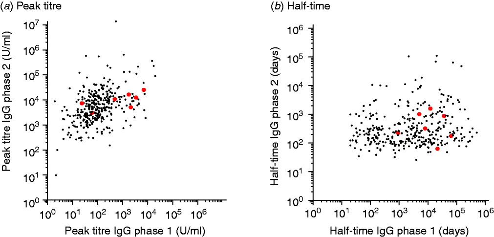
Fig. A1 [colour online]. Scatterplots of (a) peak titres and (b) half-times of IgG phase 1 and 2 antibodies for presumed chronic (grey) and non-chronic patients (black).

Fig. A2. Specificity and sensitivity of discrimination by peak titre by means of a binary mixture of normal distributions. Receiver operating characteristic (ROC) diagrams shown for the most likely (maximum likelihood) components, and 95% uncertainty interval (grey area). Also shown are levels for peak titres and half-times corresponding to the charted sensitivities and specificities (numbers along the graphs).

Fig. A3 [colour online]. IgG phase 1 and 2 titres by age (<40, 40–60, >60 years) at 0–3, 4–6, 7–9, 10–12, and >12 months following symptom onset.
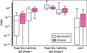
Fig. A4 [colour online]. Distribution of the odds for each patient of falling into the ‘positive’ category (cf. Fig. 4). Assessment of uncertainty in the classification by using a (Markov chain) Monte Carlo sample of fitted longitudinal responses, fitting a binary normal mixture to each individual (posterior) set of peak titres and half-times, and calculating odds over all patients in all fitted mixtures.


