


1. Introduction
Developing countries are highly vulnerable to current and future climate change (Parker, Reference Parker2006; Jongman et al., Reference Jongman, Winsemius, Aerts, de Perez, van Aalst, Kron and Ward2015). Apart from mitigating climate change, there is a need to increase adaptation efforts. Besides structural measures, such as seawalls or dikes, adaptation efforts can include ecosystem-based adaptation (EbA) measures. EbA uses biodiversity and ecosystem services (ES) as part of an adaptation strategy, and includes the sustainable management and restoration of ecosytems to help people adapt to the adverse effects of climate change (Secretariat of the Convention on Biological Diversity, 2009). Moreover, EbA could play a role in the achievement of several Sustainable Development Goals and in compliance to the Sendai Framework for Disaster Reduction, policies that are at the heart of current climate adaptation discussions. Next to its adaptation potential, EbA can prevent or revert ongoing environmental degradation that is threatening human health and life-support systems (Gupta et al., Reference Gupta, Hurley, Grobicki, Keating, Stoett, Baker, Guhl, Davies and Ekins2019; UN Environment, 2019). However, in spite of its potential benefits, current investment in EbA is limited; for instance, less than 1 per cent of total investments in water resources management is spent on ecosystem-based solutions (WWAP/UN-Water, 2018).
To guide investments and to make well-informed decisions on the implementation and design of EbA, there is a need for accurate estimation of the welfare effects of these measures. Stated preference valuation studies can fill this gap by providing information to decision makers on the economic value of the ES that are affected by the EbA measures. The results of these studies, however, are subject to criticism concerning challenges that are specific to developing countries, such as language barriers, differences in cultural context, and comparatively limited use of money as a form of income or medium of exchange (Whittington, Reference Whittington2002; Alam, Reference Alam2006; Christie et al., Reference Christie, Fazey, Cooper, Hyde and Kenter2012; Gibson et al., Reference Gibson, Rigby, Polya and Russell2016).
In stated preference valuation studies, it is common practice to incorporate a monetary payment, such as a monthly contribution to a fund or increases in tax payments. This payment vehicle is required for the calculation of willingness to pay (WTP). In a developing country context, however, a lack of market integration and dependence on subsistence livelihoods implies that many households may have low monetary incomes, and hence using a monetary payment vehicle can lead to a number of interrelated problems regarding WTP (Alam, Reference Alam2006; Kenter et al., Reference Kenter, Hyde, Christie and Fazey2011; Gibson et al., Reference Gibson, Rigby, Polya and Russell2016). First, the resulting WTP values might be an underestimation because respondents do not have the financial resources required to express their preferences for the ES. Second, limited incomes and lack of familiarity with money payments for goods and services in general, and ES in particular, may result in methodological issues such as non-attendance or protesting behaviour (Gibson et al., Reference Gibson, Rigby, Polya and Russell2016). Third, due to the previous two problems, the results of a valuation study using a monetary payment vehicle might fail to accurately represent certain groups in society, such as subsistence or poorer households, due to their (missing) relation with money (Alam, Reference Alam2006; Gibson et al., Reference Gibson, Rigby, Polya and Russell2016).
This problem stems from households in developing countries facing relatively tight monetary constraints, although they are not necessarily poor in terms of time and natural resources. Moreover, WTP is a function of a person's wealth rather than monetary income and, especially in developing countries, non-monetary goods may be a significant component of someone's wealth. Alternative payment vehicles that have therefore been trialed in developing country contexts include bags of rice (Shyamsundar and Kramer, Reference Shyamsundar and Kramer1996) and meals (Diafas et al., Reference Diafas, Barkmann and Mburu2017). The most popular alternative to a monetary payment vehicle, however, is payment in terms of time (e.g., Hardner, Reference Hardner1996; Kamuanga et al., Reference Kamuanga, Swallow, Sigué and Bauer2001; Hung et al., Reference Hung, Loomis and Thinh2007; O'Garra, Reference O'Garra2009; Abramson et al., Reference Abramson, Becker, Garb and Lazarovitch2011; Casiwan-Launio et al., Reference Casiwan-Launio, Shinbo and Morooka2011; Rai and Scarborough, Reference Rai and Scarborough2013; Vondolia et al., Reference Vondolia, Eggert, Navrud and Stage2014; Gibson et al., Reference Gibson, Rigby, Polya and Russell2016; Pondorfer and Rehdanz, Reference Pondorfer and Rehdanz2018; Vondolia and Navrud, Reference Vondolia and Navrud2019). In general, the studies that use time payment vehicles find that this payment vehicle is highly accepted by respondents, and is often preferred over money payments (Kamuanga et al., Reference Kamuanga, Swallow, Sigué and Bauer2001; Alam, Reference Alam2006; Hung et al., Reference Hung, Loomis and Thinh2007; O'Garra, Reference O'Garra2009; Abramson et al., Reference Abramson, Becker, Garb and Lazarovitch2011; Casiwan-Launio et al., Reference Casiwan-Launio, Shinbo and Morooka2011; Rai and Scarborough, Reference Rai and Scarborough2013; Vondolia et al., Reference Vondolia, Eggert, Navrud and Stage2014).
However, there are also several problematic issues with using time as a payment vehicle. One that especially stands out is the conversion of time to money values. This step is required for the estimation of monetary WTP estimates that can be used in cost benefit analyses. So far, stated preference studies in developing countries that convert time into money have mostly applied a generic market wage rate as the conversion rate (Alam, Reference Alam2006; O'Garra, Reference O'Garra2009; Vondolia et al., Reference Vondolia, Eggert, Navrud and Stage2014; Gibson et al., Reference Gibson, Rigby, Polya and Russell2016). This approach is often criticized due to heterogeneity in wages and values of time (Czajkowski et al., Reference Czajkowski, Giergiczny, Kronenberg and Englin2019; Lloyd-Smith et al., Reference Lloyd-Smith, Abbott, Adamowicz and Willard2019) as well as because respondents might intend to invest leisure time rather than working time. Rai and Scarborough (Reference Rai and Scarborough2013) and Abramson et al. (Reference Abramson, Becker, Garb and Lazarovitch2011) both estimate values of time that are lower than the market wage rate by calculating the opportunity cost of labor from discrete choice experiments that included both types of payment. Consequently, some studies used a so-called leisure rate based on the study by Cesario (Reference Cesario1976), which finds that the value of leisure time is between 25–50 per cent of the wage rate, and is being applied in the literature as 1/3 of the wage rate (O'Garra, Reference O'Garra2009; Casiwan-Launio et al., Reference Casiwan-Launio, Shinbo and Morooka2011). However, there are more recent studies that show that the value of leisure time can be much higher than 1/3 of the wage rate and differs per, for instance, income group and employment situation (Feather and Shaw, Reference Feather and Shaw1999; Alvarez-Farizo et al., Reference Alvarez-Farizo, Hanley and Barberán2001; Larson and Shaikh, Reference Larson and Shaikh2004; Larson et al., Reference Larson, Shaikh and Layton2004; Lee and Kim, Reference Lee and Kim2005; Jara-Díaz et al., Reference Jara-Díaz, Munizaga, Greeven, Guerra and Axhausen2008).
Only a few of those studies that convert the obtained time values into money thereafter compare the WTP estimates that result from both time and money payment vehicles (Alam, Reference Alam2006; O'Garra, Reference O'Garra2009; Casiwan-Launio et al., Reference Casiwan-Launio, Shinbo and Morooka2011; Vondolia et al., Reference Vondolia, Eggert, Navrud and Stage2014; Gibson et al., Reference Gibson, Rigby, Polya and Russell2016). These studies have drawn varying conclusions regarding the differences in WTP estimates resulting from time and money payment vehicles. Of the studies that used a generic market wage rate to convert time into money, two find higher WTP estimates for the time payment vehicle (Alam, Reference Alam2006; O'Garra, Reference O'Garra2009), one finds comparable WTP estimates (Gibson et al., Reference Gibson, Rigby, Polya and Russell2016) and one finds lower estimates for the time payment vehicle (Vondolia et al., Reference Vondolia, Eggert, Navrud and Stage2014). One study applied an individual-specific daily income and found comparable WTP distributions for both payment vehicles (Tilahun et al., Reference Tilahun, Vranken, Muys, Deckers, Gebregziabher, Gebrehiwot, Bauer and Mathijs2015). Then, for the comparisons that were made using a generic leisure rate based on Cesario (Reference Cesario1976), Casiwan-Launio et al. (Reference Casiwan-Launio, Shinbo and Morooka2011) found higher WTP estimates for the time payment vehicle while O'Garra (Reference O'Garra2009) found comparable WTP estimates. In conclusion, the literature is inconclusive about the differences in WTP across time and money payment vehicles and the conclusion can also differ depending on the time-to-money conversion rate that is applied.
This study is the first to conduct a stated preference valuation study in the context of the implementation of EbA measures in a developing country context and compare the WTP estimates of time and money payment vehicles using six conversion rates. These conversion rates include the commonly applied generic market wage rate and five individual-specific time-to-money conversion rates. These five conversion rates include individual-specific wage rates, two different leisure rates and two weighted values of time. The results add to the limited literature about how WTP estimates differ across time and money payment vehicles and on the use of time-to-money conversion rates, information that is crucial for the estimation of accurate welfare effects of EbA measures. The results can be used by stated preference practitioners to improve the quality of information provided to decision-makers and to guide investments in EbA.
The remainder of the paper is structured as follows. Section 2 outlines the study sites included in this research and the methods that are applied. Section 3 describes the results, and section 4 provides a discussion of the results and draws conclusions.
2. Study sites and methods
2.1 Study sites
Vietnam is an Asian developing country that is currently experiencing rapid exploitation of natural resources, climate change impacts and population growth. Vietnam is furthermore considered as one of the most vulnerable countries with respect to climate-related hazards (e.g., Dasgupta et al., Reference Dasgupta, Laplante, Meisner, Wheeler and Yan2009). This study focusses on the province of Thùa Thiên-Hu$\acute{\hat{{\rm e}}}$ , a coastal province in Central Vietnam, where frequent flood events – a total of 40 between 1975 and 2005 (Bubeck et al., Reference Bubeck, Botzen, Suu and Aerts2012) – have resulted in high damage costs and loss of life, and are expected to increase in frequency. In November 2007, typhoon Damrey caused a flood that resulted in the loss of nine lives and US$36 million in damages (KTTV, 2017; Vietnam News, 2017).
Therefore, with the broader purpose of examining the benefits of investing in EbA measures, two study sites within Thùa Thiên-Hu$\acute{\hat{{\rm e}}}$ province (see figure 1) were selected for implementation of community-led EbA measures as part of the Global Resilience Partnership Water Window. The first is an urban study site, the old town of Hu$\acute{\hat{{\rm e}}}$
 City, and the second is a coastal study site, Quảng Lợi commune in the coastal district of Quảng Đi$\grave{\hat{\rm e}}$
 n. In both sites, the community was involved in the design of the adaptation measures and community events were organized to communicate the benefits and management aspects of the implemented measures.Footnote 1
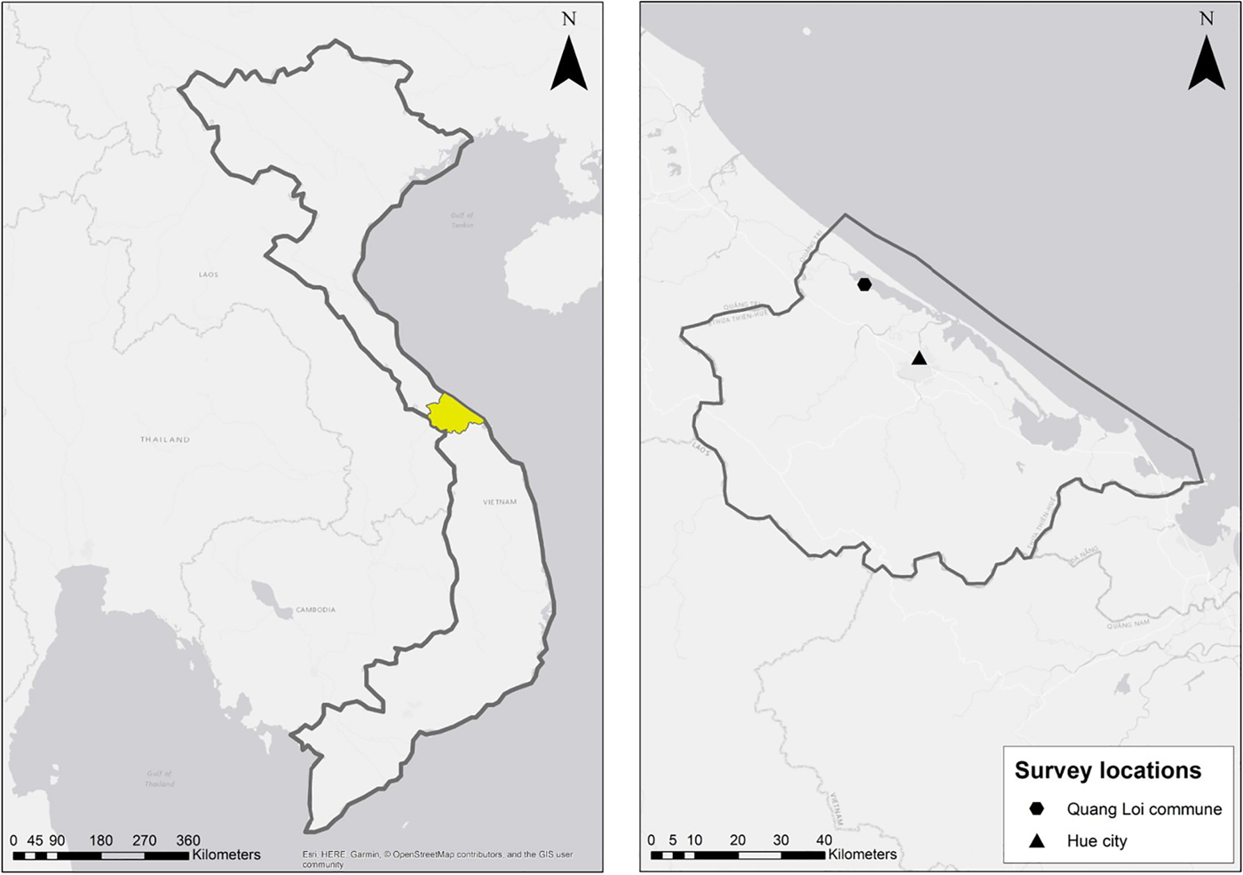
Figure 1. Location of Thùa Thiên-Hu$\acute{\hat{{\rm e}}}$ province and the case study sites Hu$\acute{\hat{{\rm e}}}$
 City (16°28′41.8′′N 107°34′49.2′′E) and Quảng Lợi commune (16°37′24.8′′N 107°27′24.1′′E).
Adjacent to Quảng Lợi commune, in the Tam Giang lagoon, a mangrove forest is being restored by replanting mangroves so as to create a buffer against storm and flood events. Simultaneously, the mangroves are also expected to increase the abundance of seafood, improve the overall water quality, provide erosion control, attract tourists, and positively influence rice and aquaculture production. Many of Thùa Thiên-Hu$\acute{\hat{{\rm e}}}$ 's coastal communities suffer from poverty resulting from unstable livelihoods and insufficient resources to recover from disasters. Mangrove restoration can potentially provide additional means to improve income security.
In the old town of Hu$\acute{\hat{{\rm e}}}$ City, a network of existing urban ponds are being restored to increase drainage capacity, similarly aimed at reducing flood and storm damages. Currently the connections between the ponds are blocked, which means the water flow is limited or stopped completely. Ancillary benefits are a cooling effect, improved aesthetics, suitability for recreation activities, tourist attraction, and increases in aquaculture and lotus production. Hu$\acute{\hat{{\rm e}}}$
 City is located on the Perfume River and has around 350,000 inhabitants. The city is a popular tourist destination due to its historic monuments, such as the Imperial City, and earned the status of UNESCO World Heritage Site in 1993.
2.2 Methods
2.2.1 Survey approach
In order to estimate the benefits of EbA, a discrete choice experiment (DCE), embedded in a household survey, was applied. To develop the DCE and household survey, an exploratory pre-test survey was implemented first, followed by a pilot test, after which the main study was conducted. In preparation for the field work, a team of 14 local enumerators, consisting of staff from Centre for Social Research and Development (CSRD) and students from Hu$\acute{\hat{{\rm e}}}$ University, received a four-day training.
Data collection took place between June and September 2017. For each test, 80 respondents were surveyed. For the main study, 505 respondents were interviewed in the coastal as well as the urban study site. In each site, the sampling frame consisted of an estimate of the number of households. Although an official list of households was not available, community leaders were able to provide a reliable estimate for the sampling procedure. The target was to interview household heads or their partners. Respondents were asked to respond on their own behalf, although some questions focused on the entire household, including questions related to food consumption, income and income sources, and resource extraction. In both study sites, areas were selected that evidently benefited from the restoration activites. In Hu$\acute{\hat{{\rm e}}}$ City this includes households living in the old town near the ponds. In Quảng Lợi commune this includes households from eight villages living on the lagoon side of the road adjacent to the mangroves. In the latter, households were sampled according to each village's relative size in terms of households. Respondents were interviewed in their homes and, to ensure a representative sample, the households were randomly selected. If a household had already participated in the pilot survey, they were excluded from the DCE sample. The respondents were evenly divided between the experiment with a time payment vehicle and the experiment with a money payment vehicle. This was done by presenting the first respondent with a time experiment, the second with a money experiment, the third with a time experiment, and so on. Kobo Toolbox software was used to record the answers of each interview.Footnote 2 More details on the sampling approach can be found in Hudson et al. (Reference Hudson, Pham and Bubeck2019), who note that the sample is representative of the province as a whole.
2.2.2 Discrete choice experiment
The DCE is a stated preference valuation method that is used to elicit values of respondents for specified changes in a good or service. It involves asking survey respondents to make repeated choices between multi-attribute descriptions of a good or service. By observing the trade-offs that are made between attributes, it is possible to estimate their relative values. The main theoretical underpinnings of the DCE method are derived from the characteristics theory of value (Lancaster, Reference Lancaster1966) and random utility theory (McFadden, Reference McFadden and Zarembka1974; Hanley et al., Reference Hanley, Wright and Adamowicz1998). The choice experiment method attempts to measure the preferences that people have for characteristics of the goods and services they consume, which in this study are the quality and quantity of ES.Footnote 3
Pre-test survey. The pre-test survey was aimed at measuring the suitability of various payment vehicles as well as at making a selection of the most important ES that are affected by the EbA measures. To select the payment vehicles, respondents were asked to score a list of payment vehicles based on coverage, trust, acceptability and practicality (Morrison et al., Reference Morrison, Blamey and Bennett2000). In both coastal and urban study sites, the two payment vehicles that scored highest and are therefore perceived as most credible and consequential were a monthly monetary contribution to a community fund for the EbA measures and time spent on the EbA measures. The information on the most important ES was used to select the other attributes for the DCE. For the coastal area, the selected ES included protection from storms and floods, abundance of seafood in the lagoon, and tourism to the mangroves. In the urban area, protection from storms and floods, suitability for recreation, and tourism in Hu$\acute{\hat{{\rm e}}}$ City were selected as the most relevant ES. Other questions in the survey concerned the measurement of current levels of the ES enjoyed by the respondents as well as the respondents' maximum WTP via each payment vehicle, so as to obtain an initial range of maximum WTP. The answers to these questions provided input for the selection of attribute levels in the DCE.
Pilot test. To ensure consequentiality, plausible levels for the payment vehicles and ES as well as sufficient information on the handling of payments and delivery of the ES are essential (Carson and Groves, Reference Carson and Groves2007; Johnston et al., Reference Johnston, Boyle, Adamowicz, Bennett, Brouwer, Cameron, Hanemann, Hanley, Ryan, Scarpa, Tourangeau and Vossler2017). Therefore, the pilot test was implemented aimed at examining the credibility of the presented situations, clarity of the choice questions, descriptions of the attributes, and pictures used to describe the attribute levels. Moreover, the pilot test was used to estimate an initial value of time in order to relate the attribute levels of both payment vehicles in the DCE for the purpose of comparability. The pilot test choice cards included both payment vehicles as well as the three ES attributes, each of which contained four attribute levels. By including both payment vehicles in one experiment, we aimed to obtain the opportunity cost of time following Rai and Scarborough (Reference Rai and Scarborough2013). Each choice card included three options: Management A, Management B and an opt-out called ‘No Management’, for which all the attributes are at their least favorable level (i.e., low) and the payment vehicles at their most favorable level (i.e., 0). The opt-out described the current situation in the communities as based on the pre-test survey results, and was found to be credible by the respondents. The pilot also tested the remaining questions in the survey. To further ensure plausible payment levels and to estimate an initial value of time, additional questions were included asking for the respondents' maximum WTP for the restoration activities via the community fund and via the time spent on restoration activities.
Main DCE. The attribute types and attribute levels for both the coastal and urban choice experiment can be found in tables 1 and 2. Two different experiments were designed for each area, one for each payment vehicle. Due to choice formulation issues during the pilot test, which resulted in insufficient quality priors, we used an orthogonal instead of a D-efficient statistical design for the DCE, in which dominant choices were identified and adjusted. To have similar levels of payment for the time and the monetary experiments, we relate the attribute levels using a value of time obtained from the pilot survey. For this we use the pilot survey questions on maximum WTP for the restoration activities via both time and money. This value of time is calculated by dividing each respondents' WTP for the restoration activities via the community fund by the willingness to spend time on the restoration activities, and by taking the median of the resulting variable (see equation (1)). For the urban study site, this resulted in a value of time of 5,000 Vietnamese dong (VND) per hour; for the coastal study site, this was a little over VND3,000 per hour.Footnote 4 The results to these pilot survey questions were also used to decide on the payment levels in all experiments.

Table 1. Attributes and attribute levels for the coastal discrete choice experiment
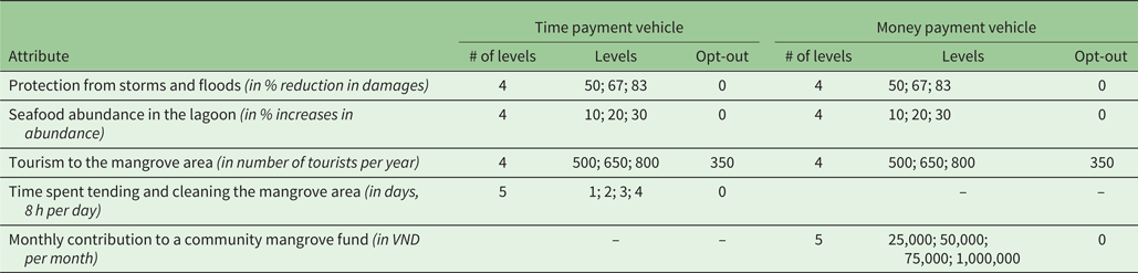
Table 2. Attributes and attribute levels for the urban discrete choice experiment
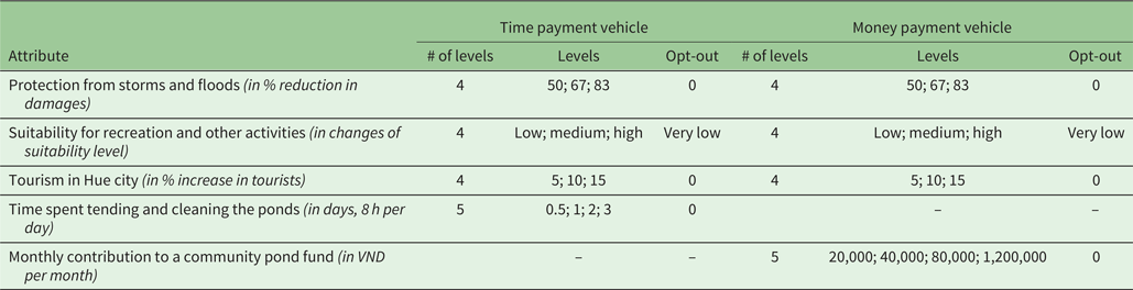
As shown in tables 1 and 2, the attributes have four levels and the payment vehicles have five. The same design was used for both the time and money payment vehicles in both coastal and urban experiments. For each experiment, 60 choice cards were generated that were divided over six versions. Three management options are presented on each choice card. The attribute levels that are included in the opt-out (No Management) were only used to describe this option and did not occur in either Management A or B.
The payment vehicles were presented to the respondents as coercive, meaning that everyone in the community would be asked to contribute time or money to the project. The payment vehicles were similar in terms of description so that the work that would be undertaken is the same whether paid for with collected money or volunteered time. This includes guarding and cleaning the restored ecosystems, building fences or look-outs, enforcing regulations and planting of trees. Vossler et al. (Reference Vossler, Doyon and Rondeau2012) note that truthful preference revelation is possible when respondents believe they have at least a weak chance of influencing the decision. To ensure consequentiality of the valuation scenario, the introductory text to the survey and framing used in the DCE laid out the project partners, funding agencies and use of the survey results. For instance, it was explained that the answers to the survey and DCE could potentially serve as input for the design of future community management plans. The pictures included on the choice cards were improved after the pilot test to ensure their effectiveness by enhancing understanding by the respondents. Vietnamese translations of the choice cards were used (see figure 2 for English examples).
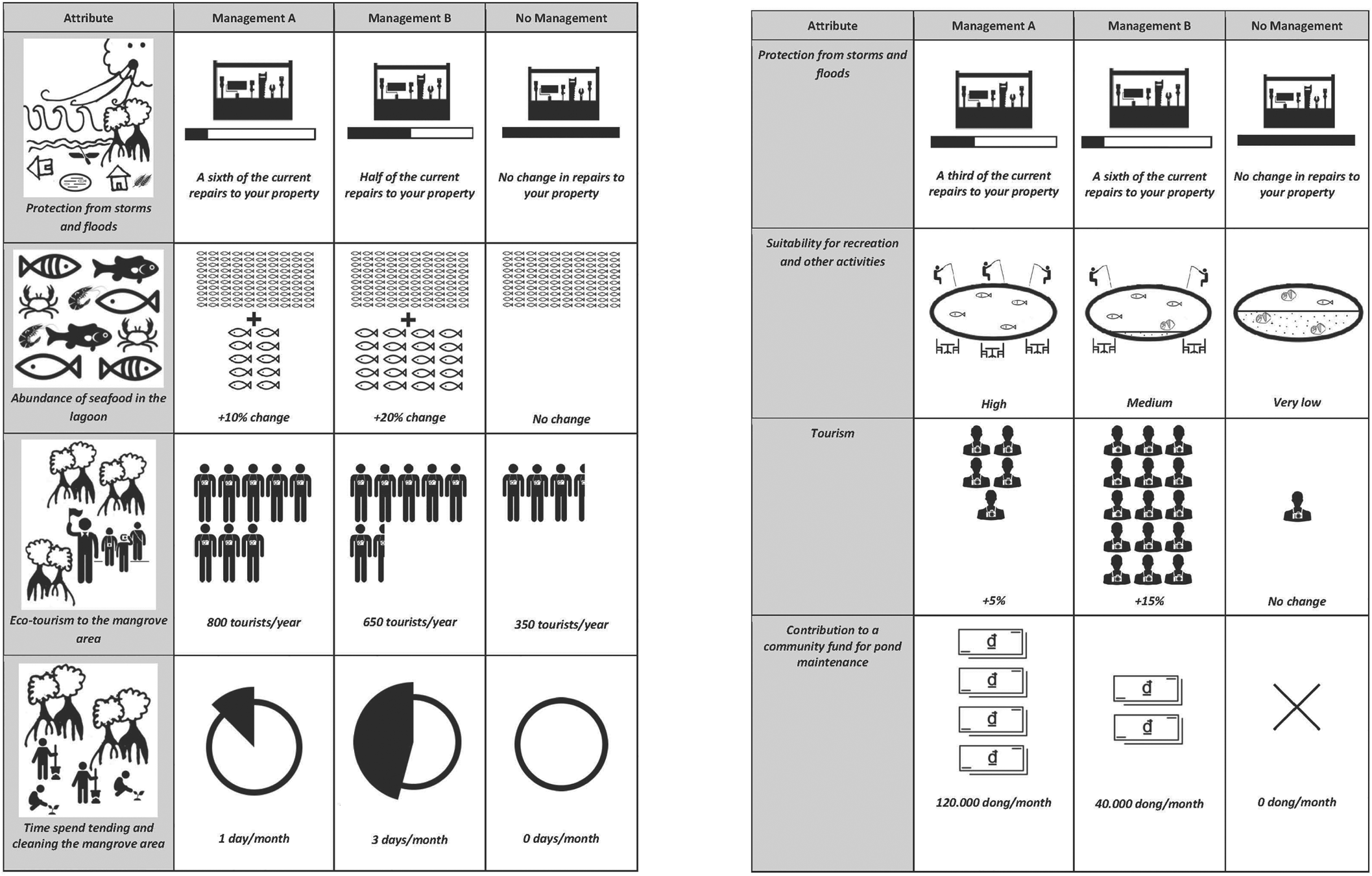
Figure 2. Example of choice cards for the coastal experiment with time payment vehicle (on the left) and the urban experiment with money payment vehicle (on the right). Note that in the urban and coastal surveys, both time and money payment vehicles were used.
Analysis of the DCE. Prior to the analysis, so-called protesters were excluded from the sample. A respondent was identified as a protester if he or she selected the ‘No Management’ option in all of the presented choices and indicated (in a follow-up question) that the motivation to do so was either a lack of trust, lack of responsibility, or unwillingness to weigh the different attributes against each other (e.g., Meyerhoff and Liebe, Reference Meyerhoff and Liebe2010; Meyerhoff et al., Reference Meyerhoff, Mørkbak and Olsen2014). In the coastal sample, nine protesters were identified of which five were part of the time payment vehicle sample and four of the money payment vehicle sample. In the urban sample, there were ten protesters in total, five in both of the samples.
The data of the DCE was analyzed using a random parameters logit (RPL) model in order to obtain individual-specific coefficients for each attribute (e.g., Brouwer et al., Reference Brouwer, Dekker, Rolfe and Windle2010; Koetse and Brouwer, Reference Koetse and Brouwer2016), implying that we can assess WTP distributions for the time experiment (WTPtime) and the money experiment (WTPmoney). All ES attributes are included in the model as continuous variables, and for each attribute 3,200 Halton draws are taken from the triangular distribution (based on Czajkowski and Budziński, Reference Czajkowski and Budziński2019). Those are restricted to positive values for the protection, seafood and recreation attributes due to theoretically expected positive preferences. For tourism the draws are taken from the triangular distribution without restriction since positive as well as negative preferences can be expected here. Triangular distributions are applied in order to be able to clearly visualize the WTP distributions for both payment vehicles and the different conversion rates, while there is a minimal reduction in model fit compared to the normal distribution. The payment vehicle values are redefined to be the negative of the variable and thereafter included in the model with a lognormal distribution and the standard deviation restricted to 0, following the new baseline model to estimate WTP as suggested by Carson and Czajkowski (Reference Carson and Czajkowski2019).
For the purpose of analyzing heterogeneity across the site-specific samples, additional models were estimated. These models include interaction terms between the payment vehicle and socio-demographic variables. The draws for the payment vehicles in these models are taken from negatively-restricted triangular distributions. Conventionally, when applying a lognormal distribution it is necessary to take the exponential of the coefficient for the payment vehicles in order to calculate WTP. This step is avoided through the application of triangular distributions and therefore makes it easier to interpret the coefficients of the interactions and the effects on WTP in these models. Moreover, for the purpose of investigating the interaction effects, this adjustment does not affect the results.
Values for the time attribute were converted to monetary values in the data set (i.e., before model estimation) by applying six alternative time-to-money conversion rates as described in the upcoming section. Using the output from the RPL models, the Krinsky and Robb (Reference Krinsky and Robb1986) procedure was applied to obtain 95 per cent confidence intervals of mean WTP estimates. Subsequently, respondent-specific parameter estimates were used to estimate a WTP for each respondent for each attribute, allowing for a clear visualization of differences in WTP distributions for the different payment vehicle experiments and for the six conversion rates. Mann-Whitney U tests were applied to assess whether WTP distributions are significantly different between the two payment vehicle experiments and across the six conversion rates.
2.2.3 Household survey
The questionnaires used in the household surveys were to a large extent identical for both study sites (i.e., coastal and urban), consisting of eight main sections including 71 questions on: (1) Dependence on ES; (2) Environmental perceptions; (3) Happiness; (4) Risk perceptions; (5) DCE and DCE debriefing; (6) Community life; (7) Flood experiences; (8) Household life and demographics. The only differences can be found in the first section, since the ES that are delivered by the mangroves differ from those delivered by the urban ponds and those questions concern the use of specific services. The questionnaire was developed in close consultation with CSRD in Hu$\acute{\hat{{\rm e}}}$ City in Vietnam, Potsdam University and Vrije University (VU) Amsterdam, and was translated into Vietnamese. During the pre-test survey and pilot, the questions were tested to check the clarity and consistency, and adjustments were made accordingly. The results of the household survey are used for the calculation of the conversion rates.
Time-to-money conversion rates. Six different types of conversion rates were used to take the required step of converting the willingness to spend time into monetary values. The first conversion rate involves the commonly applied generic market wage rate which the majority of valuation studies use. The following three are a wage and two different leisure rates, using individual-specific instead of generic wage values. The last two conversion rates are individual-specific weighted values of time that are based on additional information besides wages only.
Generic wage rate (VoT (wages, generic)): At the time of this research, the daily market wage rate for activities such as guarding, cleaning, building, planting trees and enforcement of regulations was VND130,000 in Quảng Lợi and VND150,000 in Hu$\acute{\hat{{\rm e}}}$ City. This rate is applied to each respondent in the respective study site.
Individual-specific wage rate (VoT (wages, individual)): The survey included questions on daily wages for each respondent as well as the number of hours of paid work per day. This information was used to value an eight-hour work day per respondent. This approach is comparable to the one taken by Tilahun et al. (Reference Tilahun, Vranken, Muys, Deckers, Gebregziabher, Gebrehiwot, Bauer and Mathijs2015).
Individual-specific leisure rate (VoT (leisure low) and VoT (leisure high)): Adopting the individual-specific information on daily wages as specified above, the wage rate was transformed into two leisure rates by multiplying the wage rate with leisure rate l, either 1/3 or 1.2, together presenting the lower and upper bounds of leisure values that can be found in the literature (Cesario, Reference Cesario1976; Feather and Shaw, Reference Feather and Shaw1999; Alvarez-Farizo et al., Reference Alvarez-Farizo, Hanley and Barberán2001; Larson et al., Reference Larson, Shaikh and Layton2004; Lee and Kim, Reference Lee and Kim2005; Jara-Díaz et al., Reference Jara-Díaz, Munizaga, Greeven, Guerra and Axhausen2008).
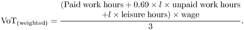
Individual-specific weighted value of time (VoT (weighted low) and VoT (weighted high)): In the calculation of this conversion rate, we assume that more than one activity could be sacrificed to contribute time and that this decision would depend on the composition of the current time spendings. Therefore, we assume that a person's value of time is not fully determined by either the value of work or by the value of leisure time, but that this value of time is instead determined by the range of work and leisure activities that a person participates in. We also assume that a person's value of time is a weighted value of the time spent on all these activities. For the calculation of this conversion rate, data on paid and unpaid hours of work (i.e., household work, subsistence activities) per day was used, as well as hours of leisure time for each respondent. For this we assume that respondents cannot exceed 18 h of work per day (including both paid and unpaid work) and that sleeping is included in leisure time. When the respondents' stated number of working hours exceeded this number, the number of hours was rescaled downwards so that the total equalled 18. A weighted value of time was calculated assuming that the value of unpaid work equals around 69 per cent of the value of leisure (based on Lee and Kim, Reference Lee and Kim2005, and Eom and Larson, Reference Eom and Larson2006). As such, the wage rate was applied for paid work time, one of the two leisure rates for the value of leisure time, and the appropriate rate depending on the selected leisure rate for unpaid work time. The value of time holds for a full day, so the 24 h were divided by three in order to obtain the value of an eight-hour day (see equation (2) for a summary of this calculation, where l refers to the applied leisure rate). For those respondents that did not have a paid job, and thus there was no information on daily wage or paid work hours, the average daily wage rate of the total sample (i.e., of all coastal or all urban respondents) was used to calculate the value of leisure time and unpaid work time for these respondents. It has been shown that unemployed and retired people also have positive values for time (Lloyd-Smith et al., Reference Lloyd-Smith, Abbott, Adamowicz and Willard2019), and therefore those respondents were included.
In order to be able to make the calculations for the six time-to-money conversion rates, 113 respondents were eliminated from the samples because of missing data, irregularities in the data, and outliers regarding the variables that were needed for the calculations. After eliminating those respondents, there were 178 and 202 respondents left in the coastal and urban time experiment samples, respectively. Regarding the analyses for the money payment vehicle, all respondents were included in these samples since there was no indication that the missing or irregular answers to the relevant survey questions reveal irregular choice behavior in the DCE.
3. Results
3.1 Data characteristics
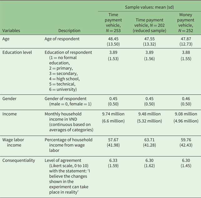
Tables 3 and 4 show the results for the key sample characteristics. In each site, Kruskal-Wallis and Chi-squared tests were applied to test for differences across the money and time samples as well as the money and reduced time samples, which are the samples that are compared in the next sections of this paper. In the coastal samples, income levels are found to be significantly higher in the time and reduced time samples, and income from wages is found to be significantly higher in the reduced time sample. No significant differences were identified across the urban samples. A follow-up question on the perceived realism of the presented changes was included in the questionnaire. The results for this question show that the respondents (on average) agree with the statement, which suggests that respondents perceived the presented scenario as consequential. The statistical tests reveal that the level of realism is significantly higher in the coastal time sample compared to the coastal money sample.
Table 3. Sample characteristics for both choice experiments in the coastal area
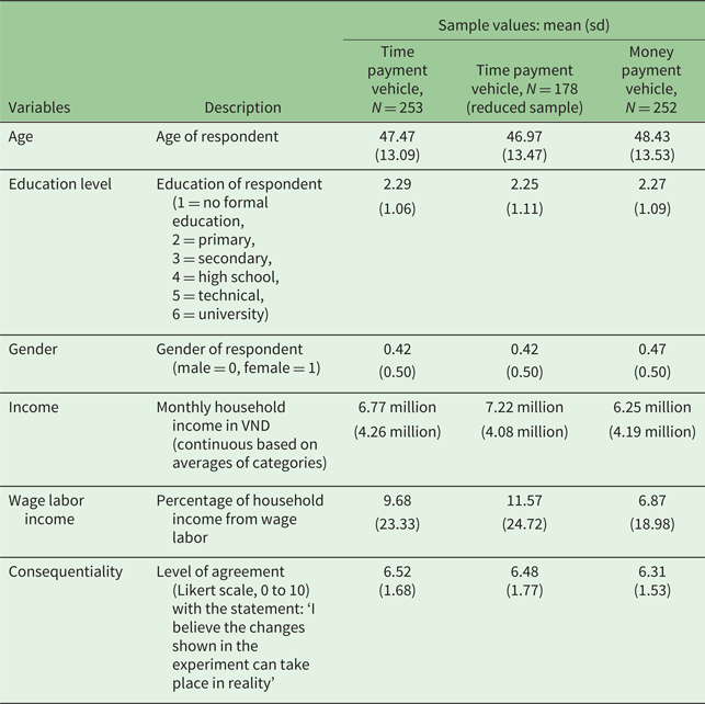
Table 4. Sample characteristics for both choice experiments in the urban area
The study sites differ in terms of socio-economic background. Table 4 shows that in the urban study site, income from wage labor on average accounts for more than 57 per cent of the household income. Many urban respondents participate in wage labor or small businesses, making wages the most important income source. Furthermore wage labor income serves as a proxy for market integration (e.g., Ensminger and Henrich, Reference Ensminger and Henrich2014; Vasco et al., Reference Vasco, Tamayo and Griess2017). The results in table 3 indicate that the level of market integration differs substantially between the urban and coastal study sites. In the coastal study site, most of the respondents (70 per cent) are fishermen and around 90 per cent of the fish catch is sold at market. The household income in this study site is therefore mostly made up of income from fisheries from the Tam Giang lagoon (54 per cent on average).
The values of time per day that were estimated through the five individual-specific conversion rates are lowest for the urban VoT (leisure low), averaging VND59,000 (~US$2.5), and highest for the coastal VoT (leisure high)), averaging VND280,000 (~US$12). The values are higher for men and higher in the coastal sample, and are positively correlated with household income. In the urban sample, the values of time are furthermore positively correlated with education and negatively correlated with age (except for VoT(weighted high)). In the coastal sample, age is negatively correlated with VoT(leisure high) and positively correlated with VoT(wages) and VoT(weighted high), while for education, negative correlations are identified with VoT(leisure high) and VoT(weighted low).
3.2 Model estimation results and mean WTP estimates
The results of the RPL models are presented in table 5 and appendix A in the online appendix. All the coefficients have the expected sign (i.e., positive for the ES and negative for the payment vehicles) and are significant at the 10 per cent level at least. As indicated by the larger coefficients, a percentage increase in seafood abundance (coastal) and a change in the level of recreation suitability (urban) are the attributes that the communities derive most utility from, followed by the specified changes in protection in the coastal area and changes in tourism in the urban area.
Table 5. Results of the RPL models for both coastal and urban experiments
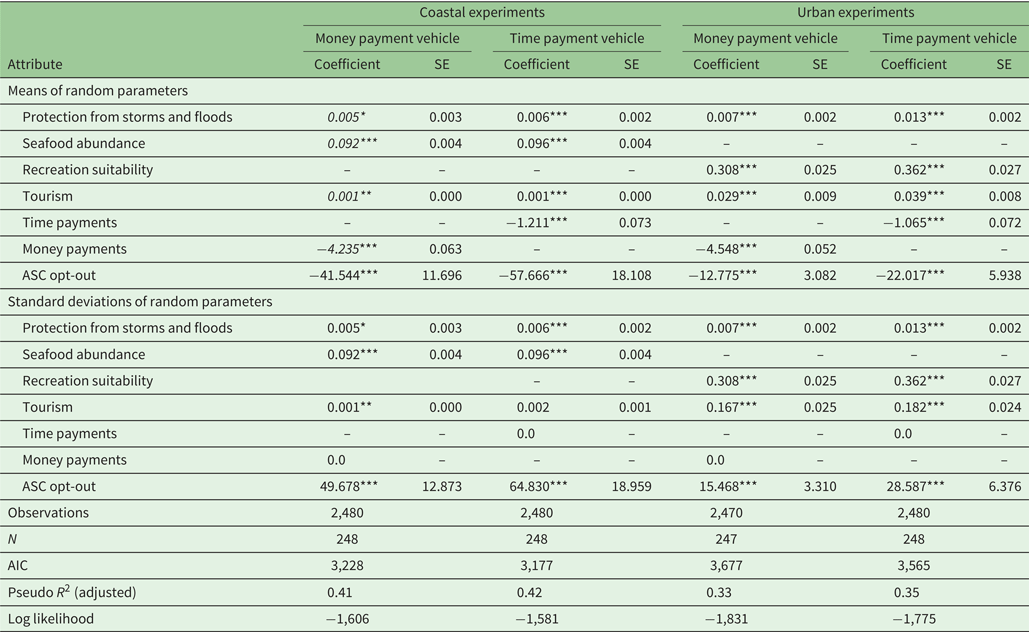
Statistical significance: *10%; **5%; ***1%.
The results of the Krinsky and Robb simulations are presented in tables 6 and 7. The numbers presented in these tables are marginal WTP for the changes in ES (i.e., the WTP per percentage increase in tourism or seafood abundance, or for an increase in the level of recreation suitability). The WTP estimates are highest when the time payments are converted with VoT(leisure high) and lowest for the money payments. The differences in WTP estimates resulting from both experiments are large, but the extent of the difference depends on the ES and conversion rate. For instance, the WTP for a given increase in seafood abundance is about 20 times larger when estimated via VoT(leisure high) compared to the WTP resulting from the money payment vehicle. The WTP for a given increase in tourism in the urban study site is about 3.5 times larger when using VoT(leisure low) compared to the money payment vehicle. There are also large differences in WTP estimates across the conversion rates. Most importantly, the differences in WTP from VoT(wages,generic) and VoT(wages,individual) differ substantially and show that not accounting for heterogeneity in wages results in an underestimation of WTP. Overall the differences in WTP estimates are substantial, depending on the payment vehicle that is used, but also the conversion rate has a strong effect on the WTP estimates that are obtained.
Table 6. Results of the Krinsky and Robb simulations for the coastal experiments in Vietnamese dong per household per month (US$1 ≈ VND23,000)
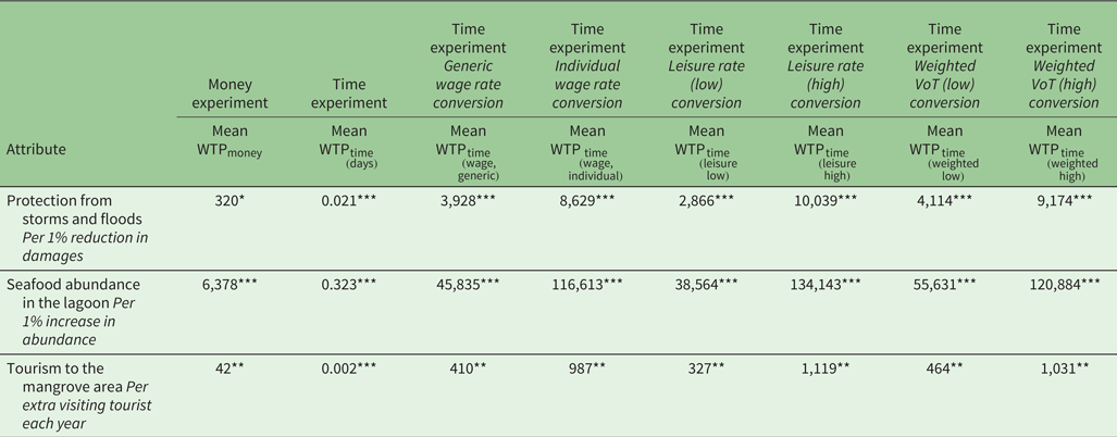
Statistical significance: *10%; **5%; ***1%.
Table 7. Results of the Krinsky and Robb simulations for the urban experiments in Vietnamese dong per household per month (US$1 ≈ VND23,000)
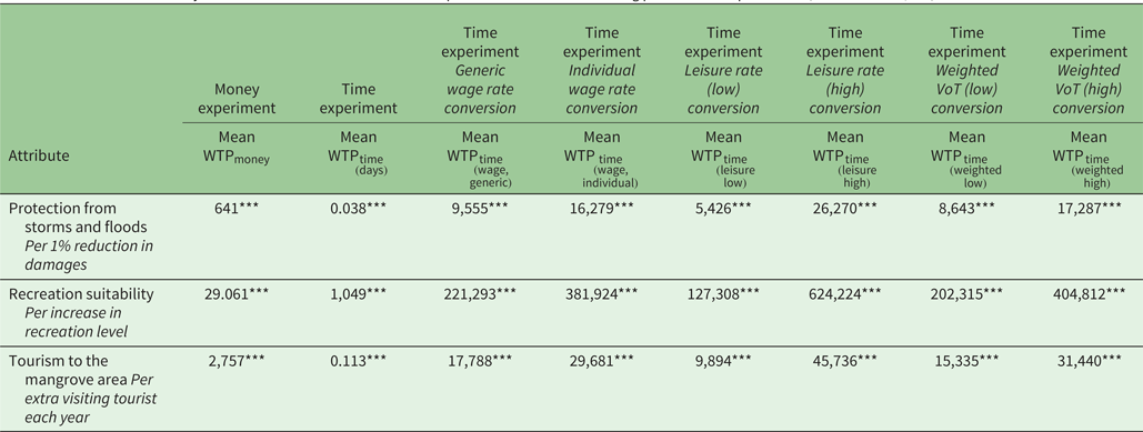
Statistical significance: ***1%.
In section 3.1, it was shown that income and income from wage labor differ significantly across the coastal money and reduced time samples. Namely, households with a higher income and more income from wage labor were overrepresented in the reduced time samples. No significant differences were identified across the urban samples. The results of the RPL models with the interactions are used to analyze the effect of the sample differences in the coastal study site. The results of these models are included in appendix B. For the income variable, a significant positive effect was found for the money payments while no significant effect was found for the time payments. Households with a higher income were under-represented in the coastal money sample, and therefore accounting for this sample difference would lead to an increase in the estimated mean WTPmoney. For the income from wage labor variable, no significant effect was found for the money payments while a significant negative effect was found for the time payments. Since households with more income from wage labor were over-represented in the time sample, accounting for this sample difference would lead to an increase in the estimated mean WTP values for all the time estimations. Both of the described results are consistent with theory. Households with a higher income are willing to pay more in terms of money and households with more income from wage labor (i.e., a higher degree of market integration) are willing to pay less in terms of time. Additionally, the models including interactions show that several other variables may explain both people's preferences and differences in WTP between time and money payment vehicles in rural and urban areas. Income, gender, age and education all have different effects (in terms of magnitude of the coefficient and/or in terms of sign) on time and money preferences in both the coastal and the urban areas.
Due to significant differences across the coastal samples, we calculate the effects on WTP when accounting for this heterogeneity as a robustness check. The difference in WTPmoney is calculated by applying the results of the interaction models in appendix B to the different sample compositions (i.e., gender, age, education level, household income and income from wage labor). Based on this calculation, we find that mean WTPmoney would increase by 1.35 per cent when the time sample composition instead of the money sample composition is applied. Similarly, WTPtime would increase by 0.63 per cent when the money sample composition instead of the time sample composition is applied. These differences in WTP are negligible compared to the minimum of 604 per cent difference in WTP that we find between both payment vehicles in the coastal area (see table 6). The identified sample differences therefore do not affect the presented conclusions on differences in WTP resulting from the time and money payment experiments.
3.3 Comparison of WTP distributions
Figure 3 presents an overview of the coastal WTP distributions that result from the calculation of respondent-specific WTP values using the RPL model outcomes. As with the results of the Krinsky and Robb simulations, higher WTP estimates are found for the time experiment for all conversion rates. Yet, these distributions appear to be more dispersed compared to the distribution of the WTP values for the money payments. As shown in figure 4, WTP distributions from experiments in the urban study site reveal comparable patterns to the coastal results in terms of the shape of WTP distributions. Compared to the coastal results, however, the distributions for all conversion rates overlap more for the tourism attribute.
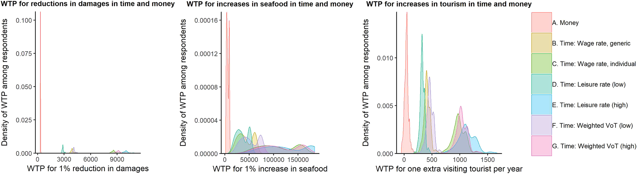
Figure 3. Willingness to pay (WTP) distributions for money and time (using six different conversion rates) for the coastal attributes ‘protection from storms and floods’ (left panel), ‘seafood abundance’ (middle panel) and ‘tourism’ (right panel).
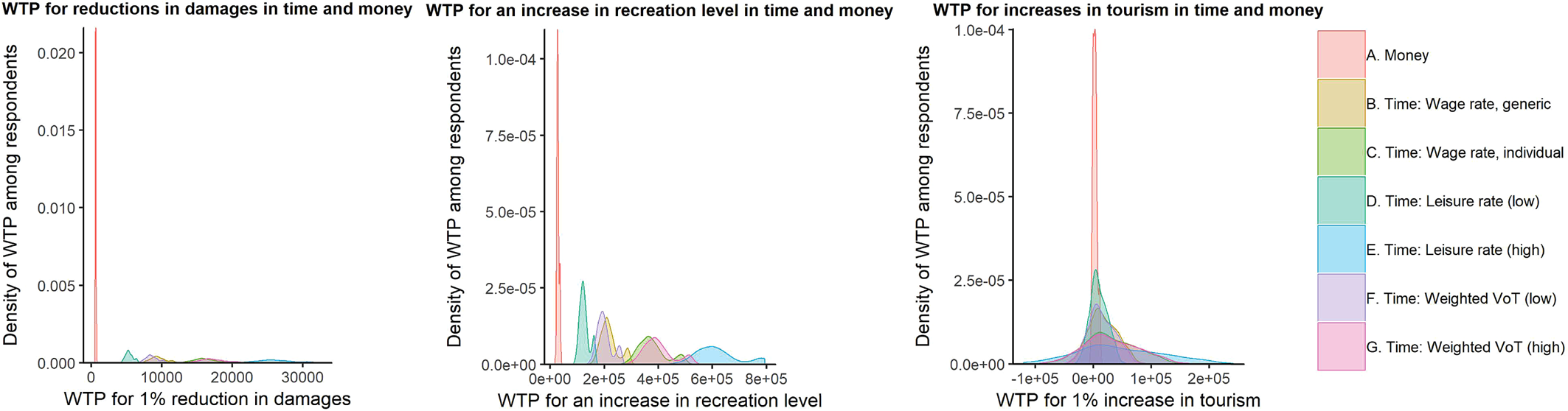
Figure 4. Willingness to pay (WTP) distributions for money and time (using six different conversion rates) for the urban attributes ‘protection from storms and floods’ (left panel), ‘recreation suitability’ (middle panel) and ‘tourism’ (right panel).
With respect to the more dispersed WTP distributions for the time experiments, no differences are found in the data related to how easy or difficult the respondents find it to make choices in the two experiments, levels of certainty about the choices or the number of protest votes. Since payment vehicles were presented as coercive, the dispersed distributions could also be explained by differences in trust, acceptability and expected cooperation between the two types of payment. Namely, issues such as free riding could play a role in the choice-making process given the public good characteristics of flood protection. A list of follow-up questions was included in the questionnaire to investigate perceived differences in these aspects across the types of payment. Three statements were included to measure expected cooperation, asking for the respondent's level of agreement (Likert scale, 0–10) regarding if all community members are able to contribute either time or money, if they expect their community members to also do so, and whether this would be easy to enforce. In both study sites, comparable means but higher variance (i.e., standard deviation) were identified in the reduced time samples for the second statement. Significantly higher means and lower variance were identified for the first and last statements (Kruskal-Wallis tests, urban: p = 0.015 and p = 0.091, coastal: p = 0.001 and p = 0.042, both respectively). In addition, a higher level and lower variance for trust in the time payments were identified in the urban study site (Kruskal-Wallis, p = 0.000) and the same result was found for acceptability concerning time contributions in the coastal study site (Kruskal-Wallis, p = 0.000). Overall the results presented in this paragraph suggest that these aspects do not explain the more dispersed WTP time distributions.
The higher dispersions are more likely to be a reflection of the fact that people have different perceptions of time, while this is less the case for money payments. There can be differences in how people perceive time used for leisure and time spent working. Moreover, working time can include farming, fishing or trading, which may all result in different values of time across respondents. This suggests that more understanding is needed on how people perceive and value time in choice experiments, potentially leading to more accurate WTP estimates and WTP distributions.
To investigate whether the WTP distributions are significantly different between the two experiments and between the different conversion rates, Mann-Whitney U tests are applied to all the different distributions per attribute. The results of these analyses show that the differences between distributions are statistically significant at the 10 per cent level at least, except for the comparison of VoT(wages,individual) and VoT(weighted high) as well as the comparison of VoT(wages,generic) and VoT(weighted low), both for the urban tourism attribute.Footnote 5 In conclusion, the graphical presentation of WTP distributions in figures 3 and 4, the Krinsky and Robb simulation results in tables 6 and 7, and results from the Mann-Whitney U tests all together reveal that the payment vehicle used, as well as the conversion rates, substantially affects WTP estimates and WTP distributions.
4. Conclusions and discussion
The main objective of this paper was to assess differences in the results of choice experiments that aim to value changes in ES as a result of EbA measures, using time and money as payment vehicles in a developing country context, and with a specific focus on the time-to-money conversion rate. There is a need to obtain more accurate WTP estimates of EbA measures in order to guide investments in EbA. The payment vehicle is an important element of a choice experiment, and stated preference studies in general, since it is required for calculating WTP. Due to subsistence livelihoods, lower incomes and limited market integration, the use of a standard money payment vehicle can be problematic in the context of developing countries and can lead to inaccurate WTP estimates (Alam, Reference Alam2006; Kenter et al., Reference Kenter, Hyde, Christie and Fazey2011; Gibson et al., Reference Gibson, Rigby, Polya and Russell2016). Time-based payment vehicles have frequently been used as an alternative to money, but only a limited number of studies have compared results from different payment vehicles, and their findings are ambiguous. In this paper, we therefore aimed to compare WTP estimates resulting from choice experiments that use time and money payment vehicles. Moreover, we address the crucial issue of how to convert time into money in more detail, especially because most previous studies only use a generic market wage rate and thus ignore heterogeneity in the value of time across respondents. In this study, we propose and apply an alternative approach which is more comprehensive and individual-specific. This approach includes applying a range of individual-specific rates alongside the commonly applied generic market wage rate. This range includes an individual-specific wage rate, two different leisures rates and two weighted values of time.
In the results of this study, the WTP estimates are higher with a time payment vehicle for all conversion rates. This finding could be interpreted to mean that a time payment vehicle performs better by allowing respondents to make choices that fully reflect their preferences. These findings correspond to those from a number of previous studies where higher WTP values were found in experiments using time payment vehicles (Alam, Reference Alam2006; Casiwan-Launio et al., Reference Casiwan-Launio, Shinbo and Morooka2011) but also contrasts with the opposite and inconclusive findings of others which include differing conclusions depending on the conversion rate (O'Garra, Reference O'Garra2009; Vondolia et al., Reference Vondolia, Eggert, Navrud and Stage2014; Gibson et al., Reference Gibson, Rigby, Polya and Russell2016). The more dispersed distributions that are found for the converted time values are in line with previous studies that identified increased confidence intervals and uncertainty in time experiments (Larson et al., Reference Larson, Shaikh and Layton2004; Vondolia and Navrud, Reference Vondolia and Navrud2019).
In contrast to previous studies, we are the first to apply five alternative conversion rates that are all individual-specific next to the commonly applied generic market wage rate. We find that applying a generic instead of individual-specific market rate results in an underestimation of WTP, aligning with the findings presented in Tilahun et al. (Reference Tilahun, Vranken, Muys, Deckers, Gebregziabher, Gebrehiwot, Bauer and Mathijs2015). We argue that the weighted value of time is a more suitable conversion rate than the rates widely applied in the literature. However, there are some uncertainties related to our conversion approaches. A concern related to the use of a daily wage is that people in developing countries might not work a set number of days per week or might participate in seasonal work. At the same time, many might work in informal settings such as trading. They therefore do not receive a formal wage and thus appear in the data as a respondent without earnings. Additional individual-specific information could therefore be used to refine the conversion rates and better capture the differences in perceptions of time, possibly leading to more accurate WTP estimates. A second concern relates to the applied wage fractions for the estimation of leisure and unpaid work time values. These fractions are based on the range found in previous studies, of which none was conducted in a developing country context, while differences in these factors across the developed and developing world could be expected.
Based on our findings we have four recommendations for stated preferences studies that aim to estimate the welfare effects of EbA in developing countries. First, we encourage practitioners of stated preference studies to consider using a time payment vehicle in developing country contexts. The payment vehicle is highly accepted, as indicated by the positive values and limited protest votes recorded in the data set, and results in higher WTP estimates, possibly because respondents can express their preferences more freely. Second, we encourage future studies that use a time payment vehicle to apply individual-specific time-to-money conversion rates to account for heterogeneity in time values across respondents. Third, we show that converted time values can differ substantially, based on the conversion rate; we therefore want to highlight the need for sensitivity analyses when converted time values are used in cost benefit analyses, for instance by providing a lower and upper range estimate based on different conversion rates. Fourth, due to the challenges faced when converting time to money, we also suggest presenting time values supplementary to the converted and thus monetary values in the final results of stated preference studies. For the purpose of solely selecting a suitable EbA measure, time values are just as informative and do not include the added uncertainties that come with converting time to monetary values.
There are several issues that deserve attention in further research. First, the development and application of a suitable conversion rate is an important aspect for stated preference studies that use time payments, since this conversion rate is crucial for the quality and reliability of the WTP estimates. In many studies, including this one, time values are transformed into monetary values with measures based on the wage rate. However, previous findings by Lloyd-Smith et al. (Reference Lloyd-Smith, Abbott, Adamowicz and Willard2019) and Czajkowski et al. (Reference Czajkowski, Giergiczny, Kronenberg and Englin2019) suggest that values of time depend to a large extent on other factors besides wages. Future stated preference studies that use time as the payment vehicle may focus on assessing these other factors, and by doing so derive more suitable values of time. For example, further improvement could come from detailed information on current time allocation, the monetary values that are attached to the different activities conducted by the respondent, and information on which current activity the respondent would be giving up in order to be able to contribute time. This could go hand in hand with the exploration of conversion rates that are not based on wages to start with. This type of conversion rate could be promising due to lower information needs and elimination of wage and leisure value related uncertainties.
Second, future studies may focus on investigating the drivers of the disparities in WTP estimates so that more information becomes available on when, and why, a time or money payment vehicle is more appropriate to use in certain socio-economic and cultural contexts. Gibson et al. (Reference Gibson, Rigby, Polya and Russell2016) and Casiwan-Launio et al. (Reference Casiwan-Launio, Shinbo and Morooka2011) both hint at the influence of market integration on WTP disparities, of which we also find evidence in this study. More extensive analyses and further study would be necessary to reveal and confirm the relevant factors that may underlie the conclusions presented in this paper. Preferences for time and money clearly vary across important dimensions, which could also include personal values and perceptions. Lastly, we want to invite researchers to conduct studies on the value of leisure time in developing countries, since to the best of our knowledge no such study is available yet.
Supplementary material
The supplementary material for this article can be found at https://doi.org/10.1017/S1355770X20000108.
Acknowledgements
We are grateful for funding for the ResilNam Urban and ResilNam Coastal projects from the Global Resilience Partnership through the Water Window and funding from NWO-WOTRO through the Urbanising Deltas of the World programme, project number W07.69.206. We also thank participants of the 25th Ulvön Conference and Workshop on Non-Market Valuation in Ulvön, 19–21 June 2018, for useful comments and suggestions. Thanks also to our project partners, Potsdam University and CSRD, and the students from Hu$\acute{\hat{{\rm e}}}$ University, for the fruitful collaboration and participation in the data collection activities. Finally, we thank two anonymous reviewers for suggestions and comments.


 Open access