


1 Introduction
X-ray tomography has applications in various industrial fields such as sawmill industry, where it can be used for detecting knots, rotten parts, and foreign objects in logs (Shustrov et al., Reference Shustrov, Eerola, Lensu, Kälviäinen and Haario2019; Zolotarev et al., Reference Zolotarev, Eerola, Lensu, Kälviäinen, Haario, Heikkinen and Kauppi2019). In oil and gas industry, X-ray tomography can be used to analyze drill-core rock samples for identifying pore structures (Mendoza et al., Reference Mendoza, Roininen, Girolami, Heikkinen and Haario2019) and other structural properties of rock. In chemical engineering, X-ray microtomography can be used to measure the internal structure of substances at the micrometer level (Ou et al., Reference Ou, Zhang, Lowe, Blanc, Rad, Wang, Batail, Pham, Shokri, Garforth, Withers and Fan2017). In manufacturing, it can be used in nondestructive testing (Garcea et al., Reference Garcea, Wang and Withers2018; Rotella et al., Reference Rotella, Nadot, Piellard, Augustin and Fleuriot2018), endurance testing (Piao et al., Reference Piao, Zhou, Xu and Wang2019), and dimensional metrology (Kruth et al., Reference Kruth, Bartscher, Carmignato, Schmitt, Chiffre and Weckenmann2011; Villarraga-Gómez et al., Reference Villarraga-Gómez, Herazo and Smith2019). In geotechnical engineering, X-ray microtomography can be used to measure soil properties in laboratories, while a closely related travel-time tomography can be used to measure the structure of soil and rocks from cross-borehole measurements (Ernst et al., Reference Ernst, Green, Maurer and Holliger2007). In medical engineering, applications include dental imaging (Kolehmainen et al., Reference Kolehmainen, Vanne, Siltanen, Järvenpää, Kaipio, Lassas and Kalke2006) and tumor tracking in radiotherapy (Shieh et al., Reference Shieh, Caillet, Dunbar, Keall, Booth, Hardcastle, Haddad, Eade and Feain2017).
The principle of X-ray tomography is that we transmit X-ray radiation to the object, which penetrates the object of interest over a collection of propagation paths, and the attenuated X-ray radiation is measured in a detector system (Toft, Reference Toft1996). This allows us to estimate internal properties of an unknown object given the noise-perturbed indirect measurements. However, typically, we can transmit and measure the X-rays only from a limited number of angles around the object which makes it harder to reconstruct the internal structure of the object from the measurements. The reconstruction problem is thus an inverse problem where the measurements give only a limited amount of information on the object of interest (Siltanen et al., Reference Siltanen, Kolehmainen, Järvenpää, Kaipio, Koistinen, Lassas, Pirttilä and Somersalo2003).
In order to successfully reconstruct the internals of the object from the limited number of measurements, we need to introduce additional information to the reconstruction process. In this article, we study so-called Bayesian methods (Kaipio and Somersalo, Reference Kaipio and Somersalo2005), where we introduce a statistical prior model for the possible internal structures in form of a probability distribution. This prior model encodes the information on what kind of structures are more likely and which are less likely than others. For example, a Gaussian random field prior puts higher probability for smoother structures, whereas total variation (TV), Besov, and Cauchy priors favor structures that can have sharper edges between the substructures (González, Reference González2017). The advantage of the Bayesian formulation is that it provides uncertainty quantification mechanism to the reconstruction problem, as it not only provides single reconstruction but also the error bars for the reconstruction in the form of a probability distribution (Bardsley, Reference Bardsley2012).
The Bayesian formulation of the X-ray tomography transforms the solution of the associated inverse problem to a Bayesian inference problem, and we need to use computational methods from Bayesian statistics to solve it. We use Markov chain Monte Carlo (MCMC) and optimization methods for computing conditional mean (CM) and maximum a posteriori (MAP) estimates, respectively. We consider a sawmill industry log tomography application for detecting knots, rotten parts, and foreign objects in sawmills (Shustrov et al., Reference Shustrov, Eerola, Lensu, Kälviäinen and Haario2019; Zolotarev et al., Reference Zolotarev, Eerola, Lensu, Kälviäinen, Haario, Heikkinen and Kauppi2019). As an oil and gas industry application, we have drill-core rock sample tomography for identifying pore structures (Mendoza et al., Reference Mendoza, Roininen, Girolami, Heikkinen and Haario2019).
1.1 X-ray tomography as a Bayesian statistical inverse problem
Reducing the number of measurements tends to add artefacts to the tomographic reconstruction. This means that we need to carefully evaluate the accuracy of the reconstruction for different levels of sparsity. For this kind of problems, a typical approach is to deploy Bayesian statistical inversion techniques in the sense of Kaipio and Somersalo (Reference Kaipio and Somersalo2005). Bayesian inversion is the theory and practical data analysis of noisy indirect measurements within the Bayesian estimation framework. Following Toft (Reference Toft1996), X-ray radiation measured at single detector pixel over a given propagation path is
 $$ {y}_{\theta, s}=\iint \mathcal{X}\left({x}_1,{x}_2\right)\delta \left(s-{x}_1\cos \theta -{x}_2\sin \theta \right){dx}_1{dx}_2+{e}_{\theta, s}=: {\mathcal{A}}_{\theta, s}\mathcal{X}+{e}_{\theta, s}, $$
where $ {y}_{\theta, s} $
is measured value at angle
$ {y}_{\theta, s} $
is measured value at angle $ \theta $
with translation
$ \theta $
with translation $ s $
and
$ s $
and $ \mathcal{X} $
is varying X-ray attenuation coefficient field inside the object of interest. For practical computations, we discretize the operation
$ \mathcal{X} $
is varying X-ray attenuation coefficient field inside the object of interest. For practical computations, we discretize the operation $ {\mathcal{A}}_{\theta, s}\mathcal{X} $
by approximating
$ {\mathcal{A}}_{\theta, s}\mathcal{X} $
by approximating $ \mathcal{X} $
with a piecewise defined function with constant values on square pixels and obtain a finite-dimensional presentation
$ \mathcal{X} $
with a piecewise defined function with constant values on square pixels and obtain a finite-dimensional presentation $ y= AX+e $
, where
$ y= AX+e $
, where $ y\in {\mathrm{\mathbb{R}}}^n $
,
$ y\in {\mathrm{\mathbb{R}}}^n $
, $ A\in {\mathrm{\mathbb{R}}}^{n\times m} $
,
$ A\in {\mathrm{\mathbb{R}}}^{n\times m} $
, $ e\in {\mathrm{\mathbb{R}}}^n $
, and
$ e\in {\mathrm{\mathbb{R}}}^n $
, and $ X\in {\mathrm{\mathbb{R}}}^m $
represent the approximated values of
$ X\in {\mathrm{\mathbb{R}}}^m $
represent the approximated values of $ \mathcal{X} $
on pixels.
$ \mathcal{X} $
on pixels.
In X-ray tomography, the noise process $ e $
is often modeled as a compound Poisson distributed noise (Whiting, Reference Whiting2002; Thanh et al., Reference Thanh, Prasath and Le Minh2019). We make a simplification and assume that
$ e $
is often modeled as a compound Poisson distributed noise (Whiting, Reference Whiting2002; Thanh et al., Reference Thanh, Prasath and Le Minh2019). We make a simplification and assume that $ e $
is zero-mean Gaussian white noise with covariance
$ e $
is zero-mean Gaussian white noise with covariance $ C={\sigma}^2I $
. As our main aim is in contrast-boosting priors, we assume that this simplification does not affect the generality of the results. The solution of the tomography problem is then an a posteriori probability density via the Bayes formula
$ C={\sigma}^2I $
. As our main aim is in contrast-boosting priors, we assume that this simplification does not affect the generality of the results. The solution of the tomography problem is then an a posteriori probability density via the Bayes formula
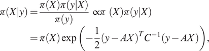 $$ \pi \left(X|y\right)=\frac{\pi (X)\pi \left(y|X\right)}{\pi (y)}\propto \pi (X)\pi \left(y|X\right)=\pi (X)\exp \left(-\frac{1}{2}{\left(y- AX\right)}^T{C}^{-1}\left(y- AX\right)\right), $$
where $ \pi (X) $
is the a priori density, that is, the probabilistic description of the unknown we know before any measurements are taken,
$ \pi (X) $
is the a priori density, that is, the probabilistic description of the unknown we know before any measurements are taken, $ \pi \left(y|X\right) $
is the likelihood density, and
$ \pi \left(y|X\right) $
is the likelihood density, and $ \pi (y) $
is a normalization constant which we can be omitted in computations.
$ \pi (y) $
is a normalization constant which we can be omitted in computations.
1.2 Literature review
Sparse-angle tomography is an ill-posed inverse problem (Natterer, Reference Natterer2001), and thus in order to have stable solutions, we need to set the prior $ \pi (X) $
. A standard choice is to use Gaussian random field priors (Bardsley, Reference Bardsley2013). They are easy to use through their analytic properties, and they are fully defined by their means and covariances. The drawback of Gaussian priors is that they are locally smoothing and thus cause contrast artefacts near sharp edges. As our objective is in reconstructing unknown objects with sharp edges, we need to choose a prior density that can model them. Such an edge-preserving, contrast-boosting prior needs to be non-Gaussian.
$ \pi (X) $
. A standard choice is to use Gaussian random field priors (Bardsley, Reference Bardsley2013). They are easy to use through their analytic properties, and they are fully defined by their means and covariances. The drawback of Gaussian priors is that they are locally smoothing and thus cause contrast artefacts near sharp edges. As our objective is in reconstructing unknown objects with sharp edges, we need to choose a prior density that can model them. Such an edge-preserving, contrast-boosting prior needs to be non-Gaussian.
When computing posterior estimates, the unavoidable non-Gaussianity of any contrast-boosting prior leads to computational complexity and high computational cost. In two-dimensional industrial tomography, with even small or moderate mesh sizes, a typical problem has around 100,000–1,000,000 unknown parameters. High dimensionality in industry poses problems, especially in time-critical applications, where speed is valued. Point estimates computed with optimization methods are natural starting points as they are computationally light. For example, the MAP estimate is fast to compute but does not unfortunately provide full uncertainty quantification.
To fully quantify uncertainty, we need to explore the whole posterior with MCMC techniques, such as Metropolis-within-Gibbs, (MwG), (see, e.g., Markkanen et al., Reference Markkanen, Roininen, Huttunen and Lasanen2019). Alternatively, we could use variational Bayes methods (Tzikas et al., Reference Tzikas, Likas and Galatsanos2008) which aim to approximate a probability distribution with a simpler one, and they are computationally cheaper than MCMC. However, variational Bayes methods have inherent approximation errors in their estimates, whereas MCMC methods theoretically do not. That is why MCMC is often preferred for uncertainty quantification. There is a growing number of MCMC algorithms for high-dimensional problems (Cotter et al., Reference Cotter, Roberts, Stuart and White2013; Law, Reference Law2014; Beskos et al., Reference Beskos, Girolami, Lan, Farrell and Stuart2017). Unfortunately, non-Gaussianity of the contrast-boosting priors breaks many of the assumptions of the function-space MCMC methods. MwG is a simple choice, but its convergence can be slow, requiring significantly long MCMC chains for accurate approximations. As an alternative, we use Hamiltonian Monte Carlo (HMC), (Neal, Reference Neal2011). It has been used for a wide range of applications, and it is well-suited for large-dimensional problems (Beskos et al., Reference Beskos, Pinski, Sanz-Serna and Stuart2011). In particular, we use the HMC variant with no-U-turn sampling (HMC-NUTS), (Hoffman and Gelman, Reference Hoffman and Gelman2014).
There are several priors which promote contrast-boosting or edge-preserving inversion. A standard choice for edge-preserving inversion is the TV prior, which is based on using $ {L}^1 $
-norms. In statistics, this method is called LASSO (least absolute shrinkage and selection operator). This method, however, has a drawback, which arises from the finiteness of the prior moments. When we make the discretization denser and denser, the TV priors converge to Gaussian priors in the discretization limit. This behavior was studied by Lassas and Siltanen (Reference Lassas and Siltanen2004), and they showed that the estimators are not consistent under mesh refinement for Bayesian statistical inverse problems. This, naturally, means that doing uncertainty quantification under TV-prior assumption is not consistent with respect to the change of the mesh.
$ {L}^1 $
-norms. In statistics, this method is called LASSO (least absolute shrinkage and selection operator). This method, however, has a drawback, which arises from the finiteness of the prior moments. When we make the discretization denser and denser, the TV priors converge to Gaussian priors in the discretization limit. This behavior was studied by Lassas and Siltanen (Reference Lassas and Siltanen2004), and they showed that the estimators are not consistent under mesh refinement for Bayesian statistical inverse problems. This, naturally, means that doing uncertainty quantification under TV-prior assumption is not consistent with respect to the change of the mesh.
Recently, several hierarchical models, which promote more versatile behaviors, have been developed. These include, for example, deep Gaussian processes (Dunlop et al., Reference Dunlop, Girolami, Stuart and Teckentrup2018; Emzir et al., Reference Emzir, Lasanen, Purisha, Roininen and Särkkä2020), level-set methods (Dunlop et al., Reference Dunlop, Iglesias and Stuart2017), mixtures of compound Poisson processes and Gaussians (Hosseini, Reference Hosseini2017), and stacked Matérn fields via stochastic partial differential equations (Roininen et al., Reference Roininen, Girolami, Lasanen and Markkanen2019). The problem with hierarchical priors is that in the posteriors, the parameters and hyperparameters may become strongly coupled, which means that vanilla MCMC methods become problematic and, for example, reparameterizations are needed for sampling the posterior efficiently (Chada et al., Reference Chada, Lasanen and Roininen2019; Monterrubio-Gómez et al., Reference Monterrubio-Gómez, Roininen, Wade, Damoulas and Girolami2020). In level-set methods, the number of levels is usually low because experiments have shown that the method deteriorates when the number of levels is increased.
Here, we utilize a different approach and make the prior non-Gaussian by construction without hierarchical modeling or compromising on uncertainty quantification. The first choice is to utilize priors based on Besov $ {\beta}_{p,q}^s $
norms (Lassas et al., Reference Lassas, Saksman and Siltanen2009). These priors are constructed on wavelet basis, typically Haar wavelets, and they have well-defined non-Gaussian discretization limit behavior. Besov priors have been utilized in a number of studies for Bayesian inversion (see, e.g., Niinimäki, Reference Niinimäki2013). The problem with Besov priors is the structure of wavelets and the truncation of the wavelet series. The coefficients of the wavelets are random but actually not interchangeable, since their decay is necessary for convergence of the series. That typically means that we make an unnecessary and strong prior assumption for edge locations based on wavelet properties, for example, consider a one-dimensional inverse problem on domain (0,1), we prefer an edge at 1/4 over an edge at 1/3 for Haar wavelets.
$ {\beta}_{p,q}^s $
norms (Lassas et al., Reference Lassas, Saksman and Siltanen2009). These priors are constructed on wavelet basis, typically Haar wavelets, and they have well-defined non-Gaussian discretization limit behavior. Besov priors have been utilized in a number of studies for Bayesian inversion (see, e.g., Niinimäki, Reference Niinimäki2013). The problem with Besov priors is the structure of wavelets and the truncation of the wavelet series. The coefficients of the wavelets are random but actually not interchangeable, since their decay is necessary for convergence of the series. That typically means that we make an unnecessary and strong prior assumption for edge locations based on wavelet properties, for example, consider a one-dimensional inverse problem on domain (0,1), we prefer an edge at 1/4 over an edge at 1/3 for Haar wavelets.
One possibility is to use $ \alpha $
-stable prior fields, see Samorodnitsky and Taqqu (Reference Samorodnitsky and Taqqu1994). Another type of
$ \alpha $
-stable prior fields, see Samorodnitsky and Taqqu (Reference Samorodnitsky and Taqqu1994). Another type of $ \alpha $
-stable priors can be constructed similarly to Besov priors. They use Karhunen-Loève (KL) type expansions instead of wavelet expansions but replace Gaussian coefficients in KL expansions with
$ \alpha $
-stable priors can be constructed similarly to Besov priors. They use Karhunen-Loève (KL) type expansions instead of wavelet expansions but replace Gaussian coefficients in KL expansions with $ \alpha $
-stable coefficients. For KL expansions, see Berlinet and Thomas-Agnan (Reference Berlinet and Thomas-Agnan2004), and for stable field expansions, see Sullivan (Reference Sullivan2017). Third option is to use pixel-based approaches (Bolin, Reference Bolin2014; Markkanen et al., Reference Markkanen, Roininen, Huttunen and Lasanen2019; Mendoza et al., Reference Mendoza, Roininen, Girolami, Heikkinen and Haario2019), which cover also some
$ \alpha $
-stable coefficients. For KL expansions, see Berlinet and Thomas-Agnan (Reference Berlinet and Thomas-Agnan2004), and for stable field expansions, see Sullivan (Reference Sullivan2017). Third option is to use pixel-based approaches (Bolin, Reference Bolin2014; Markkanen et al., Reference Markkanen, Roininen, Huttunen and Lasanen2019; Mendoza et al., Reference Mendoza, Roininen, Girolami, Heikkinen and Haario2019), which cover also some $ \alpha $
-stable random walks. The family of
$ \alpha $
-stable random walks. The family of $ \alpha $
-stable processes contains both KL expansions and pixel-based approaches, but one should note that the different approaches lead to different statistical objects. We stress that both approaches lead to well-posedness of the inverse problem. In this paper, we shall utilize certain pixel-based approaches and limit the discussion to the Cauchy difference priors, which is a special case
$ \alpha $
-stable processes contains both KL expansions and pixel-based approaches, but one should note that the different approaches lead to different statistical objects. We stress that both approaches lead to well-posedness of the inverse problem. In this paper, we shall utilize certain pixel-based approaches and limit the discussion to the Cauchy difference priors, which is a special case $ \alpha =1 $
.
$ \alpha =1 $
.
1.3 Contribution and organization of this work
The contributions of this paper are twofold, first of all, we make a large-scale numerical comparison for the X-ray tomography problem with different Gaussian and non-Gaussian (TV, Besov, Cauchy) prior assumptions. For the log and drill-core tomography applications, our paper shows the tomographic imaging limits, that is, when building the actual industrial tomography systems, we know the minimum number of measurements and noise levels with which we can attain reconstructions with predefined accuracy. This minimizes the number of components, and thus the cost, needed in the imaging system but, at the same time, ensures operational accuracy. Secondly, we apply a carefully designed HMC algorithm to the high-dimensional non-Gaussian inverse problem. In particular, we show its applicability for the sparse-angle tomography problem. Also, studying HMC chain mixing and sampling from over high-dimensional non-Gaussian posteriors is a new contribution.
The rest of this paper is organized as follows: In Section 2, we review Gaussian, TV, Besov, and Cauchy priors. In Section 3, we introduce the necessary MwG and HMC tools. In Section 4, we have two synthetic case studies: Three dimensional-imaging of logs in sawmills and drill-core tomography problem. Finally, in Section 5, we conclude the study and make some notes on future developments.
2 Random field priors
For Gaussian, TV, and Besov priors, we write the priors as $ \pi (X)\propto \exp \left(-G(X)\right) $
, where
$ \pi (X)\propto \exp \left(-G(X)\right) $
, where $ G(X) $
is
$ G(X) $
is $ {L}^2 $
-norm of differences of
$ {L}^2 $
-norm of differences of $ X $
for the Gaussian case,
$ X $
for the Gaussian case, $ {L}^1 $
-norm of differences for TV, and Besov
$ {L}^1 $
-norm of differences for TV, and Besov $ {\mathrm{\mathcal{B}}}_{p,q}^s $
-norm for a wavelet expansion with random coefficients
$ {\mathrm{\mathcal{B}}}_{p,q}^s $
-norm for a wavelet expansion with random coefficients $ {X}_1,\dots, {X}_m $
for Besov case. We will describe these distributions below and their respective
$ {X}_1,\dots, {X}_m $
for Besov case. We will describe these distributions below and their respective $ G(X) $
. In the following, we will describe separately the Cauchy prior, as it is based on another type of construction.
$ G(X) $
. In the following, we will describe separately the Cauchy prior, as it is based on another type of construction.
2.1 Gaussian prior
Let us assume a zero-mean Gaussian prior, which is fully defined with one of the following choices,
 $$ G(X)=\frac{1}{2}{X}^T{\Sigma}^{-1}X=\frac{1}{2}{X}^T QX=\frac{1}{2}{X}^T{L}^T LX=\frac{1}{2}{(LX)}^T LX, $$
where $ \Sigma $
is the covariance matrix,
$ \Sigma $
is the covariance matrix, $ Q $
is the precision matrix, and
$ Q $
is the precision matrix, and $ L $
is a square-root (e.g., Cholesky factor) of the precision matrix. Common choices are exponential and squared exponential covariances, Matérn covariances, and Brownian motion covariance. Different choices lead to different kinds of presentations, for example, squared exponential leads to full matrices for all
$ L $
is a square-root (e.g., Cholesky factor) of the precision matrix. Common choices are exponential and squared exponential covariances, Matérn covariances, and Brownian motion covariance. Different choices lead to different kinds of presentations, for example, squared exponential leads to full matrices for all $ \Sigma, Q,L $
, but with certain choices, the Matérn covariances have sparse
$ \Sigma, Q,L $
, but with certain choices, the Matérn covariances have sparse $ Q,L $
matrices due to the Markov property (Roininen et al., Reference Roininen, Girolami, Lasanen and Markkanen2019).
$ Q,L $
matrices due to the Markov property (Roininen et al., Reference Roininen, Girolami, Lasanen and Markkanen2019).
Two-dimensional difference priors can be obtained by choosing $ L $
to be a discretization of the following operator equation
$ L $
to be a discretization of the following operator equation $ \nabla \mathcal{X}=\mathcal{W} $
, where
$ \nabla \mathcal{X}=\mathcal{W} $
, where $ \mathcal{W}={\left({\mathcal{W}}_1,{\mathcal{W}}_2\right)}^T $
with two statistically independent white noise random fields
$ \mathcal{W}={\left({\mathcal{W}}_1,{\mathcal{W}}_2\right)}^T $
with two statistically independent white noise random fields $ {\mathcal{W}}_1 $
and
$ {\mathcal{W}}_1 $
and $ {\mathcal{W}}_2 $
. Thus, we have
$ {\mathcal{W}}_2 $
. Thus, we have $ LX=W $
for the discrete presentation, which we will solve in the least-squares sense. We note that the precision matrix
$ LX=W $
for the discrete presentation, which we will solve in the least-squares sense. We note that the precision matrix $ Q={L}^TL $
is not invertible, thus this is an improper prior, but if we impose zero-boundary conditions, we have a proper prior. For X-ray tomography, zero-boundary conditions are natural choices, as typically the domain of interest is larger than the object of interest, and thus putting zero-boundary is justified. Now, let us denote by
$ Q={L}^TL $
is not invertible, thus this is an improper prior, but if we impose zero-boundary conditions, we have a proper prior. For X-ray tomography, zero-boundary conditions are natural choices, as typically the domain of interest is larger than the object of interest, and thus putting zero-boundary is justified. Now, let us denote by $ {X}_{i,j} $
, the unknown at pixel
$ {X}_{i,j} $
, the unknown at pixel $ \left(i,j\right) $
. As a summation formula with zero-boundary conditions, we can write the prior then as
$ \left(i,j\right) $
. As a summation formula with zero-boundary conditions, we can write the prior then as
 $$ {G}_{\mathrm{Gauss}}(X)={G}_{\mathrm{pr}}(X)+{G}_{\mathrm{boundary}}(X)=\sum \limits_{i=1}^I\sum \limits_{j=1}^J\left(\frac{{\left({X}_{i,j}-{X}_{i-1,j}\right)}^2}{\sigma_{\mathrm{pr}}^2}+\frac{{\left({X}_{i,j}-{X}_{i,j-1}\right)}^2}{\sigma_{\mathrm{pr}}^2}\right)+\sum \limits_{i,j\in \mathrm{\partial \Omega }}\frac{X_{i,j}^2}{\sigma_{\mathrm{boundary}}^2}, $$
where by $ \mathrm{\partial \Omega } $
, we mean the boundary indices of the discretized domain
$ \mathrm{\partial \Omega } $
, we mean the boundary indices of the discretized domain $ \Omega $
,
$ \Omega $
, $ {\sigma}_{\mathrm{pr}}^2 $
is regularization parameter, and
$ {\sigma}_{\mathrm{pr}}^2 $
is regularization parameter, and $ {\sigma}_{\mathrm{boundary}}^2 $
zero-boundary parameter.
$ {\sigma}_{\mathrm{boundary}}^2 $
zero-boundary parameter.
2.2 Total variation prior
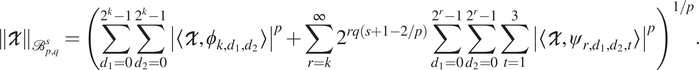
Similarly to the Gaussian prior, we can write a two-dimensional TV prior with
 $$ {G}_{\mathrm{TV}}(X)={G}_{\mathrm{pr}}(X)+{G}_{\mathrm{boundary}}(X)=\sum \limits_{i=1}^I\sum \limits_{j=1}^J\alpha \left(\left|{X}_{i,j}-{X}_{i-1,j}\right|+\left|{X}_{i,j}-{X}_{i,j-1}\right|\right)+\sum \limits_{i,j\in \mathrm{\partial \Omega }}{\alpha}_{\mathrm{boundary}}\left|{X}_{i,j}\right|, $$
where $ \alpha, {\alpha}_{\mathrm{boundary}} $
are regularization parameters. We note that in statistics, these distribution are often called Laplace distributions. This form of TV prior is anisotropic. According to González et al. (Reference González, Kolehmainen and Seppänen2017), it can be shown that an isotropic form is obtained when we choose
$ \alpha, {\alpha}_{\mathrm{boundary}} $
are regularization parameters. We note that in statistics, these distribution are often called Laplace distributions. This form of TV prior is anisotropic. According to González et al. (Reference González, Kolehmainen and Seppänen2017), it can be shown that an isotropic form is obtained when we choose
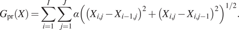 $$ {G}_{\mathrm{pr}}(X)=\sum \limits_{i=1}^I\sum \limits_{j=1}^J\alpha {\left({\left({X}_{i,j}-{X}_{i-1,j}\right)}^2+{\left({X}_{i,j}-{X}_{i,j-1}\right)}^2\right)}^{1/2}. $$
Using higher-order TV priors would be possible (Liu et al., Reference Liu, Huang, Selesnick, Lv and Chen2015), but often the basic first-order TV prior is selected because it preserves sharp edges within the reconstruction much better. The major drawback of TV prior is that due to its finite moments, the prior is not discretization-invariant, and it resembles Gaussian difference prior on dense enough meshes. It is notable that MAP estimate and the CM estimate differ drastically of each other in the limit (Lassas and Siltanen, Reference Lassas and Siltanen2004). While the inconsistency is not desirable, the prior is still used in many practical applications. In the numerical experiments, we use anisotropic TV prior. We apply Charbonnier approximation to make the gradient of the posterior differentiable everywhere (Charbonnier et al., Reference Charbonnier, Blanc-Feraud, Aubert and Barlaud1997).
2.3 Besov prior
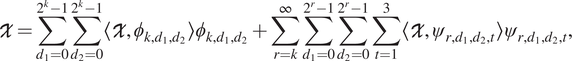
Gaussian and TV priors are based on Gaussian and Laplace distributions. Besov priors are based on the wavelet coefficients of the reconstruction. The coefficients are calculated by discrete wavelet transform (DWT) (Lassas et al., Reference Lassas, Saksman and Siltanen2009). The discrete wavelet transform decomposes the reconstruction into approximation and detail coefficients. For detailed treatise on Besov priors, see (Niinimäki, Reference Niinimäki2013). Besov prior for $ X $
derives from wavelet expansion for function
$ X $
derives from wavelet expansion for function $ \mathcal{X} $
 $$ \mathcal{X}=\sum \limits_{d_1=0}^{2^k-1}\sum \limits_{d_2=0}^{2^k-1}\left\langle \mathcal{X},{\phi}_{k,{d}_1,{d}_2}\right\rangle {\phi}_{k,{d}_1,{d}_2}+\sum \limits_{r=k}^{\infty}\sum \limits_{d_1=0}^{2^r-1}\sum \limits_{d_2=0}^{2^r-1}\sum \limits_{t=1}^3\left\langle \mathcal{X},{\psi}_{r,{d}_1,{d}_2,t}\right\rangle {\psi}_{r,{d}_1,{d}_2,t}, $$
and its Besov norm is
 $$ {\left\Vert \mathcal{X}\right\Vert}_{{\mathrm{\mathcal{B}}}_{p,q}^s}={\left(\sum \limits_{d_1=0}^{2^k-1}\sum \limits_{d_2=0}^{2^k-1}{\left|\left\langle \mathcal{X},{\phi}_{k,{d}_1,{d}_2}\right\rangle \right|}^p+\sum \limits_{r=k}^{\infty }{2}^{rq\left(s+1-2/p\right)}\sum \limits_{d_1=0}^{2^r-1}\sum \limits_{d_2=0}^{2^r-1}\sum \limits_{t=1}^3{\left|\left\langle \mathcal{X},{\psi}_{r,{d}_1,{d}_2,t}\right\rangle \right|}^p\right)}^{1/p}. $$
In Equation (3), $ \phi $
is the father wavelet and
$ \phi $
is the father wavelet and $ \psi $
is the mother wavelet. The subindices refer to different scales and translations of the functions (Meyer, Reference Meyer1992). We utilize the prior for Besov space
$ \psi $
is the mother wavelet. The subindices refer to different scales and translations of the functions (Meyer, Reference Meyer1992). We utilize the prior for Besov space $ {\mathrm{\mathcal{B}}}_{1,1}^1 $
, which reduces the norm into absolute sum of wavelet coefficients. Other Besov spaces than
$ {\mathrm{\mathcal{B}}}_{1,1}^1 $
, which reduces the norm into absolute sum of wavelet coefficients. Other Besov spaces than $ {\mathrm{\mathcal{B}}}_{1,1}^1 $
would be doable as well, but in those cases, the wavelet coefficients would have different weights or they would be raised to other powers than one. We use Haar wavelets as our father and mother wavelets. Similarly to the TV prior, we use Charbonnier approximation for the gradient.
$ {\mathrm{\mathcal{B}}}_{1,1}^1 $
would be doable as well, but in those cases, the wavelet coefficients would have different weights or they would be raised to other powers than one. We use Haar wavelets as our father and mother wavelets. Similarly to the TV prior, we use Charbonnier approximation for the gradient.
In practise, we compute the two-dimensional DWT of $ X $
, which is now represented as a reconstruction of size of
$ X $
, which is now represented as a reconstruction of size of $ {2}^n\times {2}^n, n\in \mathrm{\mathbb{N}} $
square pixels. The Besov prior is defined by
$ {2}^n\times {2}^n, n\in \mathrm{\mathbb{N}} $
square pixels. The Besov prior is defined by
 $$ {G}_{\mathrm{Besov}}(X)=\sum \limits_{d_1=0}^{2^k-1}\sum \limits_{d_2=0}^{2^k-1}\left|{a}_{k,{d}_1,{d}_2}\right|+\sum \limits_{r=k}^{k_{\mathrm{max}}}\sum \limits_{d_1=0}^{2^r-1}\sum \limits_{d_2=0}^{2^r-1}\sum \limits_{t=1}^3\left|{b}_{r,{d}_1,{d}_2,t}\right|. $$
Terms $ {a}_{k,{d}_1,{d}_2} $
refer to the approximation coefficients of the DWT of
$ {a}_{k,{d}_1,{d}_2} $
refer to the approximation coefficients of the DWT of $ X $
and terms
$ X $
and terms $ {b}_{r,{d}_1,{d}_2,t} $
to the corresponding detail coefficients. As DWT algorithm, we choose a matrix operator method described by Wang and Vieira (Reference Wang and Vieira2010). A more common and faster way to calculate the DWT would be to use fast wavelet transform, but we want to keep track of how changing the value of an individual pixel alters the wavelet coefficients and therefore the prior, too. This property is needed in the MwG algorithm because we propose new samples for each component of
$ {b}_{r,{d}_1,{d}_2,t} $
to the corresponding detail coefficients. As DWT algorithm, we choose a matrix operator method described by Wang and Vieira (Reference Wang and Vieira2010). A more common and faster way to calculate the DWT would be to use fast wavelet transform, but we want to keep track of how changing the value of an individual pixel alters the wavelet coefficients and therefore the prior, too. This property is needed in the MwG algorithm because we propose new samples for each component of $ X $
in a sequential manner and calculating the whole DWT every time for all the components would be too time consuming.
$ X $
in a sequential manner and calculating the whole DWT every time for all the components would be too time consuming.
Besov priors are discretization-invariant and therefore should remain consistent if the resolution is increased (Lassas et al., Reference Lassas, Saksman and Siltanen2009). Their drawback is the tendency to produce block artefacts into the point estimates: the wavelet coefficients at certain low scale are different, even though they are adjacent to each other. This makes Besov priors location-dependent, that is, they are not translation-invariant.
2.4 Cauchy prior
While the previous three priors were constructed based on different types of norms, Cauchy priors are constructed based on Cauchy walk or more profoundly general $ \alpha $
-stable random walk. These one-dimensional objects have well-defined limits, and the generalization in (Markkanen et al., Reference Markkanen, Roininen, Huttunen and Lasanen2019) to two-dimensional setting is given as a prior density
$ \alpha $
-stable random walk. These one-dimensional objects have well-defined limits, and the generalization in (Markkanen et al., Reference Markkanen, Roininen, Huttunen and Lasanen2019) to two-dimensional setting is given as a prior density
 $$ \pi (X)\propto \prod \limits_{i=1}^I\prod \limits_{j=1}^J\frac{h\lambda}{{\left( h\lambda \right)}^2+{\left({X}_{i,j}-{X}_{i-1,j}\right)}^2}\frac{h\lambda}{{\left( h\lambda \right)}^2+{\left({X}_{i,j}-{X}_{i,j-1}\right)}^2}, $$
where $ h $
is discretization step in both coordinate directions, and
$ h $
is discretization step in both coordinate directions, and $ \lambda $
is the regularization parameter. These priors have been used for X-ray tomography in oil and gas industry (Mendoza et al., Reference Mendoza, Roininen, Girolami, Heikkinen and Haario2019) and subsurface imaging (Muhumuza et al., Reference Muhumuza, Roininen, Huttunen and Lähivaara2020).
$ \lambda $
is the regularization parameter. These priors have been used for X-ray tomography in oil and gas industry (Mendoza et al., Reference Mendoza, Roininen, Girolami, Heikkinen and Haario2019) and subsurface imaging (Muhumuza et al., Reference Muhumuza, Roininen, Huttunen and Lähivaara2020).
A second formulation of the Cauchy difference prior was derived in (Chada et al., Reference Chada, Lasanen and Roininen2019). In that, the starting point was $ \alpha $
-stable sheets, which lead to difference approximations of the form
$ \alpha $
-stable sheets, which lead to difference approximations of the form
 $$ \pi (X)\propto \prod \limits_{i=1}^I\prod \limits_{j=1}^J\frac{h^2\lambda }{{\left({h}^2\lambda \right)}^2+{\left({X}_{i,j}-{X}_{i-1,j}-{X}_{i,j-1}+{X}_{i-1,j-1}\right)}^2}. $$
We note that Cauchy difference prior is theoretically justified in the discretization limit, which is not the case with TV prior. Unlike Gaussian difference prior, Cauchy difference prior favors small increments and steep transitions relatively much more. This means that Cauchy difference prior preserves edges within the lattice and does not smooth them out. A disadvantage of Cauchy difference prior is its anisotropic nature.
3 Posterior estimates
The two most common estimators drawn from the posterior density (Equation 2) are the MAP and CM estimates. For MAP estimation, we will use limited-memory BFGS (L-BFGS) optimization algorithm, which belongs to the family of quasi-Newtonian methods. For CM estimation, we use MCMC methods, as they also enable uncertainty quantification of the estimators by generating samples from the target distribution Kaipio and Somersalo (Reference Kaipio and Somersalo2005). For a detailed MCMC review, see Luengo et al. (Reference Luengo, Martino, Bugallo, Elvira and Särkkä2020).
3.1 Adaptive Metropolis-within-Gibbs
We use single-component adaptive Metropolis-Hastings (SCAM) (Haario et al., Reference Haario, Saksman and Tamminen2005), an adaptive variant of the MwG, (Brooks et al., Reference Brooks, Gelman, Jones and Meng2011) algorithm, to generate samples from the posterior distribution. At each iteration, each component of the target distribution is treated as a univariate probability distribution, while all the other component values of the distribution are kept constant. After a new value for the component is proposed, for example, using a Gaussian distributed transition from the previous value of the component, the new value is either accepted or rejected according to the Metropolis-Hastings rule. A new sample is added to the chain after all the components have been looped over. The process then continues until a fixed number of samples have been generated.
Adaptive MwG uses a Gaussian proposal distribution and adapts its proposal covariance by using previous samples. In high-dimensional distributions, it is more efficient than a Metropolis-Hastings algorithm which proposes the new values for all components at once (Raftery et al., Reference Raftery, Tanner and Wells2001).
3.2 Hamiltonian Monte Carlo
In Hamiltonian, or Hybrid, Monte Carlo (HMC), the negative logarithm of the probability density function of the target distribution is interpreted as a potential energy function of a physical system (Neal, Reference Neal2011; Betancourt, Reference Betancourt2017; Barp et al., Reference Barp, Briol, Kennedy and Girolami2018) with the target variable being the position variable of the system. Samples are generated by simulating trajectories from the physical system defined by the potential energy function and an additional momentum variable. The energy of the physical system is the sum of the potential energy and kinetic energy which is proportional to the square of the momentum. One initializes a random momentum vector, sets the position to be the last sample in the chain, and simulates a trajectory of the system using so-called symplectic integrator (Barp et al., Reference Barp, Briol, Kennedy and Girolami2018). The final position of the trajectory is then accepted or rejected into the chain using a Metropolis-Hastings rule.
An advantage of HMC is that if trajectory simulation parameters are suitable, it can sample from the posterior distribution efficiently. It also takes the correlations of the distribution components into account. Its computational complexity also scales better with the dimensionality than that of a simple Metropolis-Hastings (Neal, Reference Neal2011; Beskos et al., Reference Beskos, Pillai, Roberts, Sanz-Serna and Stuart2013) algorithm.
The trajectory simulation of HMC requires manually specifying a set of parameters, which greatly affect the efficiency of the sample generation. To cope with this problem, there is an automatic HMC algorithm called no-U-turn (NUTS) HMC (Hoffman and Gelman, Reference Hoffman and Gelman2014), which eliminates the need for manual tuning. For these reasons, we use NUTS as an alternative to MwG in our numerical experiments. However, even with automatic tuning, HMC may still struggle at sampling from multimodal (Mangoubi et al., Reference Mangoubi, Pillai and Smith2018) or heavy-tailed distributions (Livingstone et al., Reference Livingstone, Faulkner and Roberts2017). To cope with these problems, it would be possible to use methods such as Riemannian manifold HMC (Girolami and Calderhead, Reference Girolami and Calderhead2011) or continuously tempered HMC (Graham and Storkey, Reference Graham and Storkey2017) instead of the plain NUTS HMC.
4 Numerical experiments
We have two numerical experiments, the log tomography and the drill-core tomography. In log tomography, we have a foreign object inside, thus it is a high-contrast target. The second experiment is a lower-contrast target with lots of distinct regions with different attenuation coefficient. The measurement setting is the same for both test cases: We shall use X-ray tomography with parallel beam geometry. The computational grid is $ 512\times 512 $
, so we have 262,144-dimensional posterior distributions. We have additive white noise models, according to Equation (1), we fix the standard deviation of the noise to 1.5% of the maximum value of the line integrals. The parameters of each prior distribution at each measurement scenario are set using a grid search. For each prior, we select the parameter value, which gives approximately a minimum
$ 512\times 512 $
, so we have 262,144-dimensional posterior distributions. We have additive white noise models, according to Equation (1), we fix the standard deviation of the noise to 1.5% of the maximum value of the line integrals. The parameters of each prior distribution at each measurement scenario are set using a grid search. For each prior, we select the parameter value, which gives approximately a minimum $ {L}^2 $
-error between the MAP estimate and the ground truth. In the log tomography case, we use a different log slice without a high attenuation object to select the parameters. In real-life applications, we should select the parameters other means, such as setting a hyperprior distribution for the prior parameter—this will naturally introduce computational burden especially due to coupling of the unknown (Chada et al., Reference Chada, Lasanen and Roininen2019; Monterrubio-Gómez et al., Reference Monterrubio-Gómez, Roininen, Wade, Damoulas and Girolami2020). For Besov prior, we use eight levels in the DWT.
$ {L}^2 $
-error between the MAP estimate and the ground truth. In the log tomography case, we use a different log slice without a high attenuation object to select the parameters. In real-life applications, we should select the parameters other means, such as setting a hyperprior distribution for the prior parameter—this will naturally introduce computational burden especially due to coupling of the unknown (Chada et al., Reference Chada, Lasanen and Roininen2019; Monterrubio-Gómez et al., Reference Monterrubio-Gómez, Roininen, Wade, Damoulas and Girolami2020). For Besov prior, we use eight levels in the DWT.
In simulations, we shall use the four priors, and utilise L-BFGS, adaptive MwG, and HMC-NUTS. The initial points of MCMC chains are set to be the MAP estimate obtained with L-BFGS. As MCMC chain lengths, we use 500,000 samples in MwG to adapt proposal variances for each component and use those variances to generate 400,000 samples. To save memory, we thin the MwG chains by storing every 300th sample. For HMC-NUTS, we run 100 times for the dual averaging algorithm to tune the Störmer–Verlet symplectic integrator, and then we generate 4,000 samples for uncertainty quantification. For MCMC convergence analysis, we use Geweke z-score test for measuring stationarity of the chain and autocorrelation function and time $ \tau $
for checking chain mixing (Geweke, Reference Geweke1992; Roy, Reference Roy2020). We also convert the
$ \tau $
for checking chain mixing (Geweke, Reference Geweke1992; Roy, Reference Roy2020). We also convert the $ z $
-score into a two-sided
$ z $
-score into a two-sided $ p $
-value, for certain significance level comparisons. For good MCMC convergence,
$ p $
-value, for certain significance level comparisons. For good MCMC convergence, $ \tau $
should be small and
$ \tau $
should be small and $ p $
-value close to 1.
$ p $
-value close to 1.
Depending on the prior, and because in log tomography, we have a high-contrast target, the marginal and conditional posteriors turn out to be wide or even multimodal. The low-contrast drill-core tomography is in this sense an easier target, hence we quantify uncertainty only the log tomography as it is a more demanding test scenario. Thus for the drill-core tomography phantom, we only compute MAP estimators as the log tomography already showcases the capabilities of the uncertainty quantification.
4.1 Log tomography
Our test case is visualized in Figure 1, with metallic piece in black and knots in light color, and a small rotten part in near white with more smooth behavior. Besides the ground truth, we have also plotted the three-dimensional estimates, obtained by stacking two-dimensional MAP estimate slices computed with L-BFGS. We have all the four different priors, and the number of equispaced measurement angles is 10, 30, or 90. We have tabulated the peak signal-to-noise ratio (PSNR) of the reconstructions in Table 1. While all the methods seem to capture the main features in densest-data case, reducing the number of measurement causes severe artefacts with Gaussian and TV priors, and the Besov prior promotes blocky estimate. Cauchy prior captures the metallic piece even in the most difficult case, but it struggles with knots. The parameters used in the reconstructions are: For Gaussian prior, $ \sigma =10 $
for all test cases; for TV,
$ \sigma =10 $
for all test cases; for TV, $ \alpha =0.72 $
for the 10 angle case, 1.40 in 30 angle case, and 2.68 in 90 angle case; for Besov,
$ \alpha =0.72 $
for the 10 angle case, 1.40 in 30 angle case, and 2.68 in 90 angle case; for Besov, $ \alpha =1.40 $
in the 10 and 30 angle cases and 3.16 in the 90 angle case; for Cauchy,
$ \alpha =1.40 $
in the 10 and 30 angle cases and 3.16 in the 90 angle case; for Cauchy, $ {\left(\lambda h\right)}^2=0.0014 $
in the 10 angle case, 0.0040 in the 30 angle case, and 0.0317 in the 90 angle case.
$ {\left(\lambda h\right)}^2=0.0014 $
in the 10 angle case, 0.0040 in the 30 angle case, and 0.0317 in the 90 angle case.
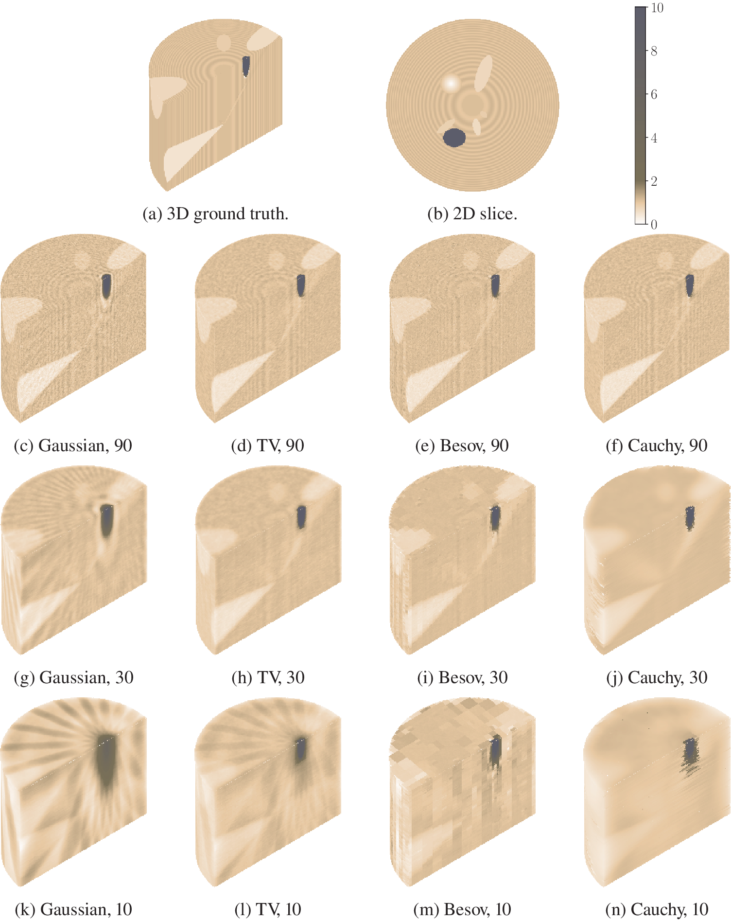
Figure 1. Log tomography: Three-dimensional and two-dimensional ground truths with knots (light material) and metallic piece (black). Three-dimensional reconstructions obtained by stacking two-dimensional maximum a posteriori (MAP) estimates with different angles and priors.
Table 1. PSNR values in decibels for the MAP and CM estimates with different priors in log tomography.
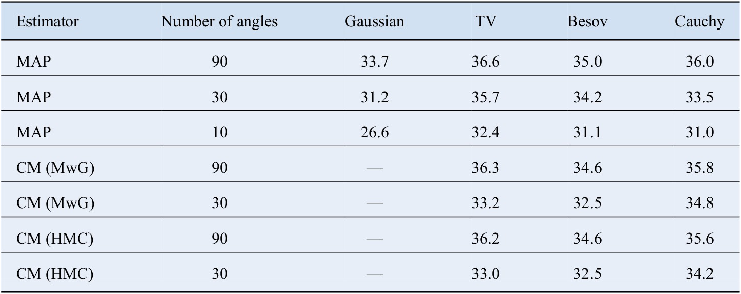
Abbreviations: CM, conditional mean; HMC, Hamiltonian Monte Carlo; MAP, maximum a posteriori; MwG, Metropolis-within-Gibbs; PSNR, peak signal-to-noise ratio; TV, total variation.
It is easier to see the effects of different priors in the two-dimensional slices in Figure 2. The densest scenario, with 90 angles, TV, and Cauchy priors produce very good MAP estimates recovering the edges. MAP estimate with Besov prior looks blocky. In the MAP estimate with Gaussian prior, the edges of the metallic object are smoothed. Reducing the number of measurement angles causes visible artefacts into MAP estimates with TV and Gaussian priors, but TV prior preserves the edges much better. Meanwhile, the rotation-dependency of Cauchy difference prior becomes apparent with coordinate-axis-aligned sharp artefacts. The Besov prior MAP estimate remains more or less consistent even if the number of angles is decreased. However, in practice, the block artefacts will spoil the MAP estimates and that is not useful in practical applications. We could decrease the number of wavelet transform levels in order to reduce blockiness or use another wavelet family.
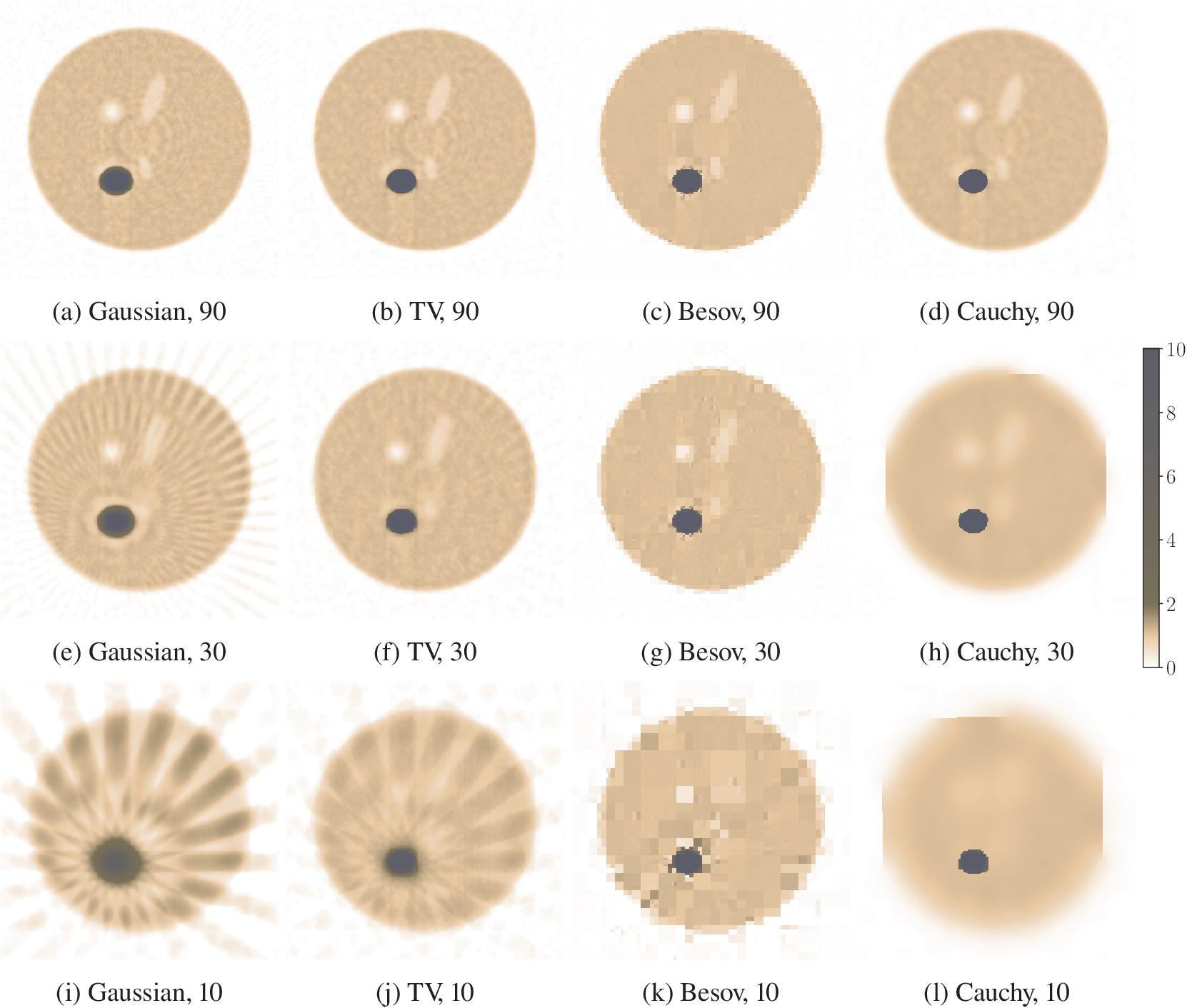
Figure 2. Log tomography: Two-dimensional maximum a posteriori (MAP) estimates with different measurement angles and prior assumptions.
In Figure 3, we have plotted the CM estimates computed with MwG and HMC. Here we skip Gaussian priors, as the CM and MAP estimates with Gaussian priors are the same. The PSNR values are tabulated in Table 1. It is notable that the CM estimate with TV prior differs noticeably from its MAP estimate (Figures 1 and 2). For high-dimensional inverse problems, it has been demonstrated by Lassas and Siltanen (Reference Lassas and Siltanen2004, figure 4) that CM estimates might be wildly oscillatory, even though the same prior produces reasonable MAP estimates. Also, the great number of scanning artefacts is notable. On the other hand, CM estimates with Cauchy difference prior have less coordinate-axis-related artefacts, and CM estimates of Besov prior are less blocky than their corresponding MAP estimates.
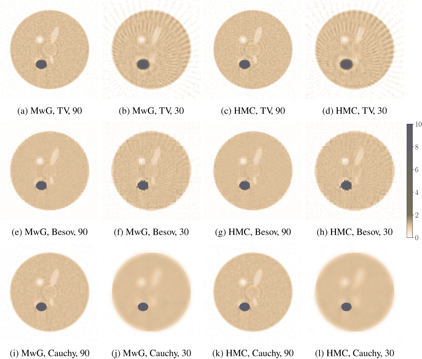
Figure 3. Log tomography: Two-dimensional conditional mean (CM) estimates with different measurement angles, prior assumptions, and samplers.
In Figure 4, we have logarithmic pixel-wise variances estimated from MwG and HMC-NUTS MCMC chains. In Table 2, we have tabulated MCMC chain convergence statistics for two different pixel locations, and the autocorrelation functions are plotted in Figure 5. For pixel $ \left(\mathrm{256,256}\right) $
, MwG has good convergence in all cases. HMC performs otherwise well, with the exception of a poor autocorrelation for the 30-angle case with Cauchy prior. The Geweke test
$ \left(\mathrm{256,256}\right) $
, MwG has good convergence in all cases. HMC performs otherwise well, with the exception of a poor autocorrelation for the 30-angle case with Cauchy prior. The Geweke test $ p $
-values are good in all cases. Pixel
$ p $
-values are good in all cases. Pixel $ \left(\mathrm{343,237}\right) $
is located at the edge of the high-attenuation object and the wood. For the 90-angle case with Cauchy prior, the marginal distribution of the posterior of that pixel is bimodal, and HMC cannot jump between the modes efficiently. This causes bad autocorrelation and
$ \left(\mathrm{343,237}\right) $
is located at the edge of the high-attenuation object and the wood. For the 90-angle case with Cauchy prior, the marginal distribution of the posterior of that pixel is bimodal, and HMC cannot jump between the modes efficiently. This causes bad autocorrelation and $ p $
-values, that is, we have serious convergence issues. 30-angle case is better in the sense of convergence of the chain, as HMC does not explore the other mode at all. In general, MwG chains with Cauchy prior mix better and have better autocorrelation values than HMC chains. However, MwG may not find all the posterior modes. This is because some of the pixels at the boundary of the high-attenuation object have much higher variance than the other boundary pixels, as seen from the variance estimates.
$ p $
-values, that is, we have serious convergence issues. 30-angle case is better in the sense of convergence of the chain, as HMC does not explore the other mode at all. In general, MwG chains with Cauchy prior mix better and have better autocorrelation values than HMC chains. However, MwG may not find all the posterior modes. This is because some of the pixels at the boundary of the high-attenuation object have much higher variance than the other boundary pixels, as seen from the variance estimates.
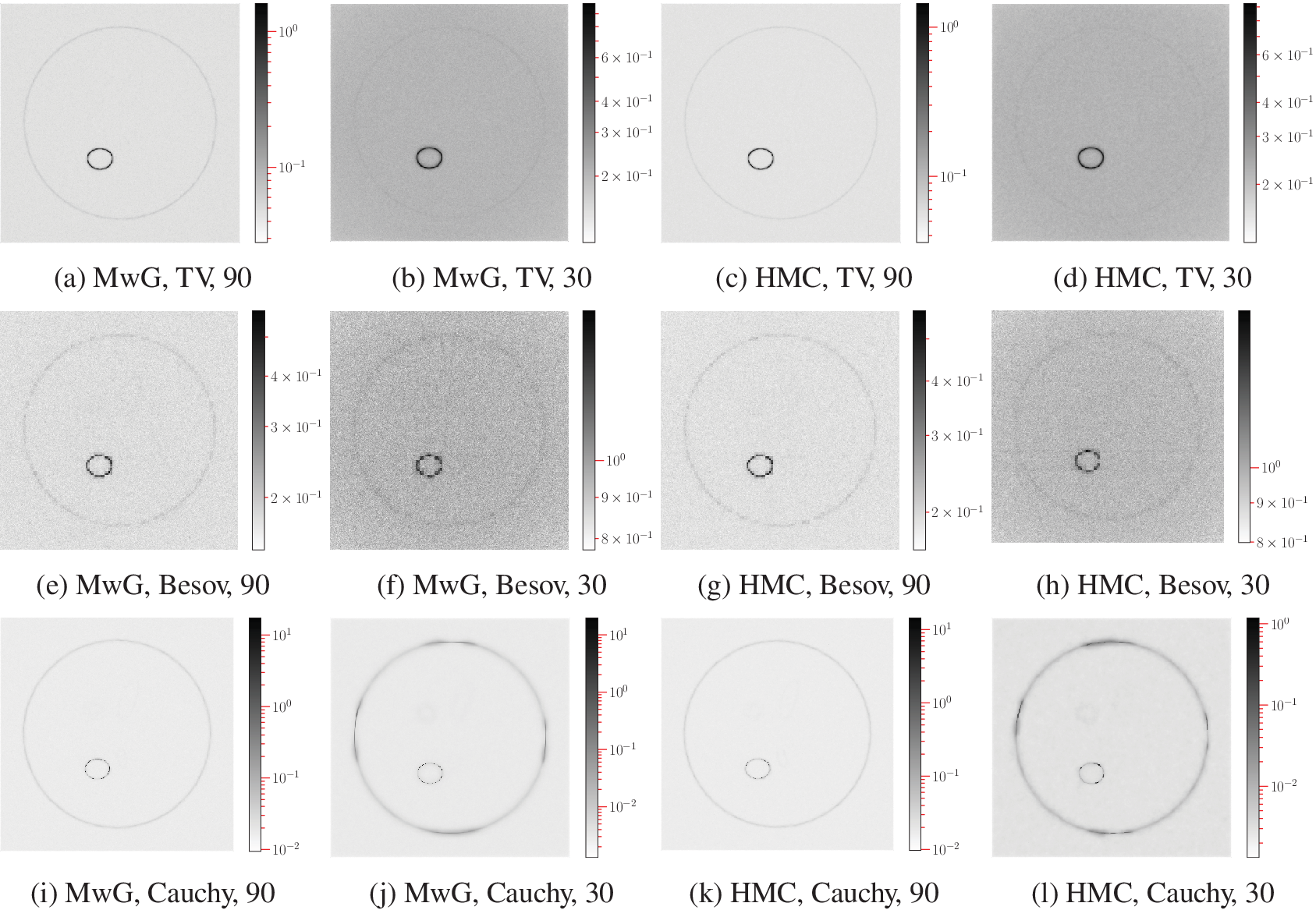
Figure 4. Log tomography pixel-wise variance estimates.
Table 2. Log tomography chain convergence estimators for two pixels with different priors and varying number of angles.

Abbreviations: HMC, Hamiltonian Monte Carlo; MwG, Metropolis-within-Gibbs; TV, total variation.
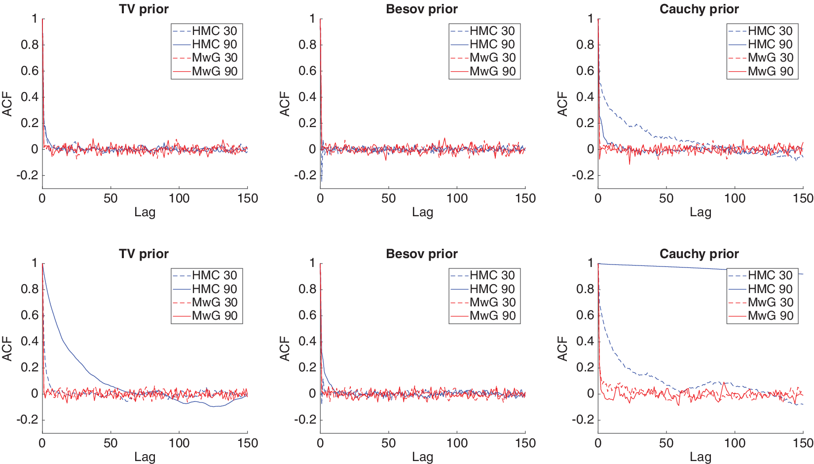
Figure 5. Log tomography Markov chain Monte Carlo (MCMC) chain autocorrelation functions for pixels $ \left(\mathrm{256,256}\right) $
(top row) and
$ \left(\mathrm{256,256}\right) $
(top row) and $ \left(\mathrm{343,237}\right) $
(bottom row).
$ \left(\mathrm{343,237}\right) $
(bottom row).
The posteriors with Cauchy prior lead to multimodal and heavy-tailed distributions, and this induces mixing issues for both methods, but particularly for HMC as it is known to underperform at sampling from such distributions (Livingstone et al., Reference Livingstone, Faulkner and Roberts2017; Mangoubi et al., Reference Mangoubi, Pillai and Smith2018). HMC-NUTS is an almost plug-and-play alternative for MwG for all other cases, except Cauchy, for which special HMC methods should be considered. HMC chain mixing can be improved by adapting a global mass matrix for the momentum by running a preliminary run for posterior variance estimation. For our high-dimensional case, local mass matrix is computationally infeasible. Tempered HMC may also enhance the algorithm (Graham and Storkey, Reference Graham and Storkey2017). For MwG tuning, we have limited chances for improvement, but, that is, robust adaptive Metropolis-Hastings could provide some further enhancements (Vihola, Reference Vihola2011).
4.2 Drill-core tomography
Here we take a simpler setting for a lower-contrast target, and we detect pores and mineralized soil within a core sample. Unlike in the log tomography experiment, the objects do not have drastically different absorption coefficient levels. However, the drill-core sample has lots of pores and soil cobs and their sizes also vary.
We demonstrate only MAP estimation, and the results are in Figure 6. At the first glance, there are no significant differences within the MAP estimates if we compare TV, Cauchy, and Gaussian difference priors to each other at 90 measurement angle scenario. Nevertheless, we consider the Cauchy and TV priors as the best ones, since they have the best PSNR values and least amount of noise, and they preserve the edges of the pores with low-and high-attenuation regions of the core sample well. If we wanted to achieve the same level of noise with Gaussian difference prior, we would end up having clearly oversmoothed MAP estimates. The PSNR values are in Table 3. Again, we use grid search to set the parameters: For Gaussian prior $ \sigma =0.37 $
and Besov prior
$ \sigma =0.37 $
and Besov prior $ \alpha =0.61 $
in all cases; for 10-angle case with TV prior
$ \alpha =0.61 $
in all cases; for 10-angle case with TV prior $ \alpha =0.1 $
and 0.37 in 30-angle case and 0.72 in 90-angle case; for 10-angle case with Cauchy prior
$ \alpha =0.1 $
and 0.37 in 30-angle case and 0.72 in 90-angle case; for 10-angle case with Cauchy prior $ {\left(\lambda h\right)}^2=1.66 $
and 0.18 in the 30-angle case and 0.55 in the 90-angle case.
$ {\left(\lambda h\right)}^2=1.66 $
and 0.18 in the 30-angle case and 0.55 in the 90-angle case.
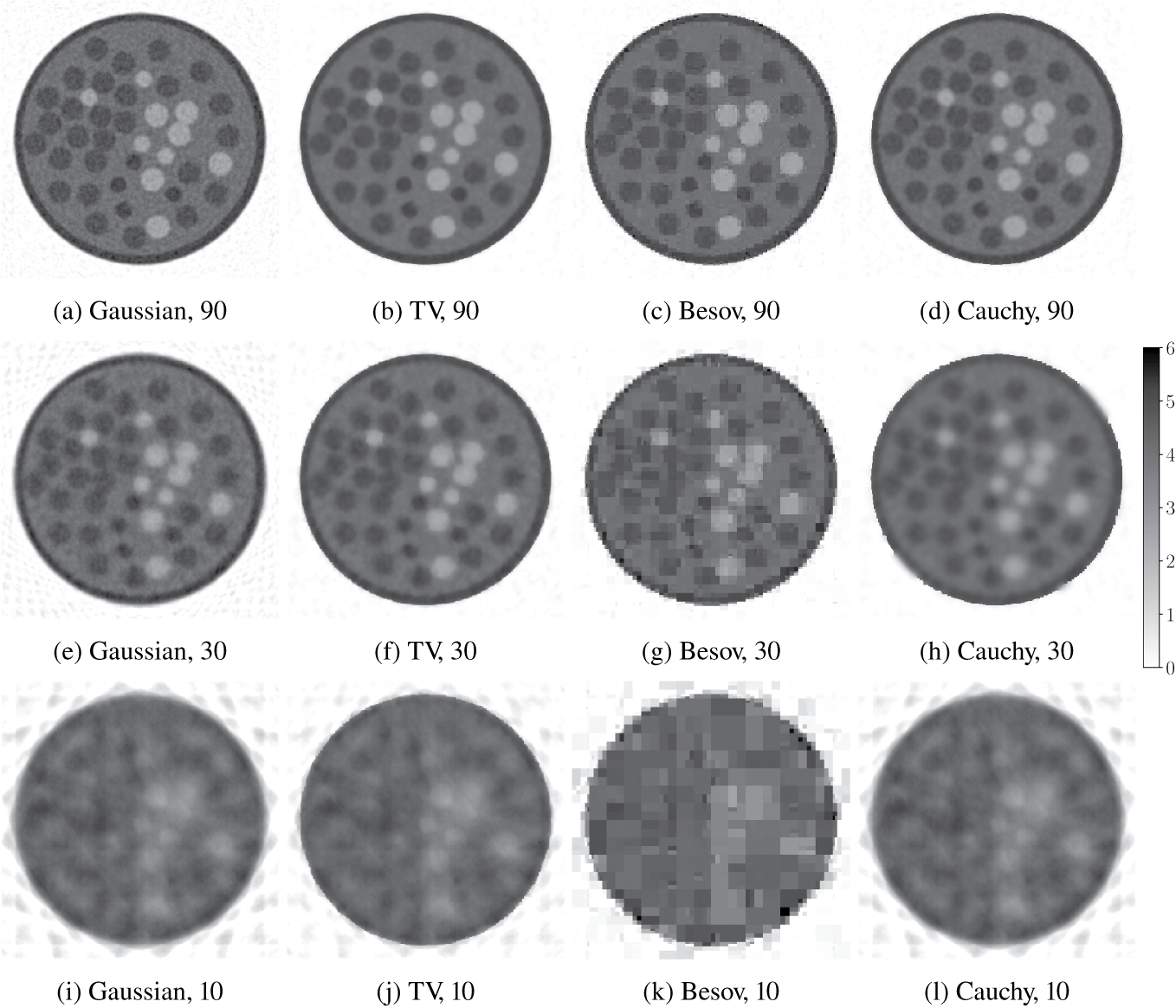
Figure 6. Drill-core maximum a posteriori (MAP) estimates for the with different measurement angles and prior assumptions.
Table 3. Drill-core tomography PSNR values in decibels for the MAP estimates with different priors.
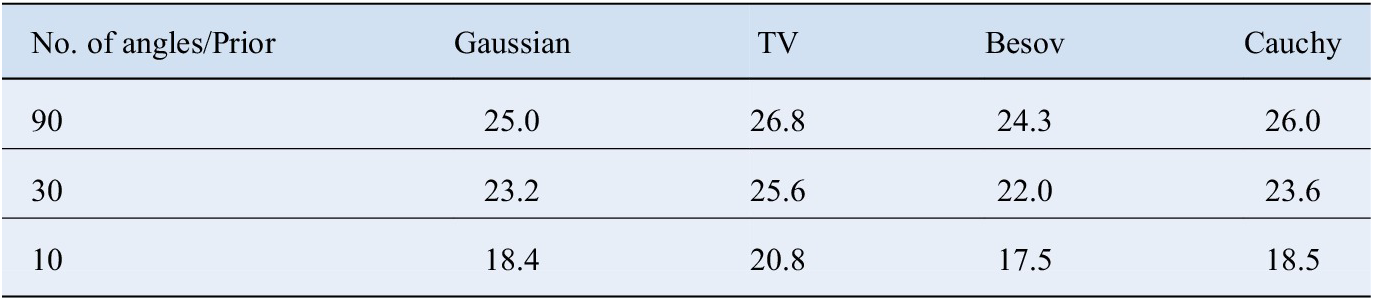
Abbreviations: MAP, maximum a posteriori; PSNR, peak signal-to-noise ratio; TV, total variation.
In the 10-angle and 30-angle scenarios, MAP estimates with Besov prior are severely ruined with block artefacts—the phantom consists of many spherical objects which are close to each other, but the wavelet coefficients of Haar family do not approximate well such details. Unlike in the log tomography, there are not so many artefacts present in the MAP estimates with Gaussian prior. In the 10-angle case, MAP estimates calculated with Gaussian, TV, and Cauchy priors are very close to each other, and neither of them can be considered superior over the others. We could try to fix the coordinate-axis dependency of Cauchy prior by introducing isotropic Cauchy prior so that we set a bivariate Cauchy distribution for differences of each pixel to their neighbors.
5 Conclusion
We have made a Bayesian inversion industrial tomography comparison study with four different priors. The targets have different contrasts, that is, sharp edges were to be reconstructed. This is a classical problem, where one needs either hierarchical or non-Gaussian models, and hence inherently computational complexity becomes a problem. The chosen methods, to use optimization or MCMC, is a balance between fast computations and uncertainty quantification. It should be noted that for many industrial applications, the computational cost is still too high, like for many dynamical systems. However, for static objects and case studies where computational time is not critical, the correctly chosen methods can significantly enhance the reconstruction results for difficult measurement geometries and targets. Systematic choice of different parameters, including mesh refinement parameters, dictate the reconstruction accuracy. In order to show the maximum possible reconstruction capabilities, we have used simple grid searches. In reality, parameter choice requires implementing some kind of a hierarchical model. This would naturally further increase computational complexity.
In all the scenarios considered, MAP estimates with Cauchy and TV priors were the best—their artefacts were mild in general and edge-preserving performance excellent. The estimates using Besov prior with Haar wavelets underperformed compared to the other priors in most cases due to the major block artefacts it tends to produce. We could decrease the block artefacts by reducing the number of DWT levels or using another wavelet family but even that cannot fix the location dependency of the prior. Likewise, we could try replacing the Cauchy prior with a bivariate Cauchy distribution to make it isotropic. For further development, applying acceptance-ratio-based adaptation in MwG and using tempered HMC would improve sampling. Other prior distributions, like general $ \alpha $
-stable priors and using hierarchical priors with possibly many layers might potentially improve the edge-preserving properties. A future avenue is also in reducing the instability by combining non-Gaussian priors to the machine-learning-based priors Adler and Öktem (Reference Adler and Öktem2018), hence possibly providing more robust methods against noise and difficult measurement geometries.
$ \alpha $
-stable priors and using hierarchical priors with possibly many layers might potentially improve the edge-preserving properties. A future avenue is also in reducing the instability by combining non-Gaussian priors to the machine-learning-based priors Adler and Öktem (Reference Adler and Öktem2018), hence possibly providing more robust methods against noise and difficult measurement geometries.
Funding Statement
This work has been funded by Academy of Finland (project numbers 326240, 326341, 314474, 321900, 313708) and by European Regional Development Fund (ARKS project A74305).
Competing Interests
The authors declare no competing interests exist.
Data Availability Statement
Codes and the synthetic data used are available openly in GitHub https://github.com/suurj/tomo/.
Authorship Contributions
Conseptualization, S.L., S.S., and L.R.; Funding acquisition, S.S. and L.R.; Methodology, J.S., M.E., S.L., S.S., and L.R.; Data visualization, J.S.; Software, J.S. and M.E.; Original draft, J.S., M.E., S.L., and L.R. All authors approved the final submitted draft.
Ethical Standards
We have followed the ethical code of conduct for research and publication of the Academy of Finland.
Acknowledgments
Authors thank Prof. Heikki Haario and Prof. Marko Laine for useful discussions.


 Open access
Comments
No Comments have been published for this article.