


Impact Statement
In this work, we analyze approaches that combine traditional knowledge-based methods to model high-dimensional chaotic systems while reducing their dimension, based on a technique called proper orthogonal decomposition (POD), with novel machine learning techniques based on echo state network (ESN). We show that a specific hybrid approach that corrects the prediction from the knowledge-based model in full state space can more accurately predict the evolution of the chaotic systems than when using either approach separately. In addition, a rigorous analysis is performed on the gain in prediction accuracy obtained depending on the base accuracy of the POD part of the hybrid approach. An interpretation on how this approach blends the POD part and the ESN part to deduce the evolution of the chaotic systems is also provided. This work provides insights that enable the wider use of a combination of traditional modeling and prediction approaches with novel machine learning techniques to obtain an improved time-accurate prediction of chaotic systems.
1. Introduction
The vast majority of physical systems, from climate and atmospheric circulation to biological systems, is often characterized by a chaotic dynamics that involves multiple spatio-temporal scales. This chaotic nature originates from complex nonlinear interactions that make the understanding and forecasting of such systems extremely challenging. Compounding this issue, many chaotic systems are high dimensional, further hindering our ability to forecast their evolutions.
To enable the quick time-accurate prediction of the evolution of such high-dimensional chaotic systems, forecasting approaches have often relied on the development of reduced-order models (ROMs) capturing the essential dynamics of the chaotic system or simplified models introducing errors stemming from modeling assumptions (Rowley and Dawson, Reference Rowley and Dawson2017; Taira et al., Reference Taira, Brunton, Dawson, Rowley, Colonius, McKeon, Schmidt, Gordeyev, Theofilis and Ukeiley2017). Among such techniques, proper orthogonal decomposition (POD) and its related extensions, spectral POD (SPOD), and dynamic mode decomposition (DMD) have been widely successful in identifying coherent structures and the relevant or most information containing modes in chaotic systems, and turbulent flows in particular (Lumley, Reference Lumley, Yaglom and Tartarsky1967; Schmid, Reference Schmid2010; Sieber et al., Reference Sieber, Paschereit and Oberleithner2016). This then allows for the retention of these most energy-conserving modes to represent the system and the truncation of the least important ones, therefore achieving a dimensional reduction of the original high-dimensional chaotic systems. Subsequently, combined with the Galerkin projection method, the dynamics of this reduced-order model can then be modeled to forecast the evolution of the chaotic systems (Berkooz et al., Reference Berkooz, Holmes and Lumley1993; Rowley et al., Reference Rowley, Colonius and Murray2004). However, such ROMs based on POD/Galerkin projection may not always provide a sufficient accuracy, especially for complex chaotic systems that can exhibit extreme events and can suffer from instability (San and Maulik, Reference San and Maulik2018; Maulik et al., Reference Maulik, Lusch and Balaprakash2021). In addition, the Galerkin projection method relies on the knowledge of the governing equations of the chaotic systems which may not always be available.
In contrast to this latter approach that requires some physical knowledge or considerations, data-driven methods from machine learning have recently shown a strong potential in learning and predicting the evolution of chaotic systems (Hochreiter, Reference Hochreiter1997; Jaeger and Haas, Reference Jaeger and Haas2004; Lukoševičius and Jaeger, Reference Lukoševičius and Jaeger2009; Brunton et al., Reference Brunton, Proctor and Kutz2016). In particular, recurrent neural networks have been used to learn the time-evolution of chaotic time series, with, for example, the use of the long short-term memory (LSTM) units (Hochreiter, Reference Hochreiter1997). This LSTM has been used to learn the dynamics of a reduced representation of a shear flow and could accurately reproduce the statistics of this nine-dimensional system (Srinivasan et al., Reference Srinivasan, Guastoni, Azizpour, Schlatter and Vinuesa2019). This system was also analyzed in Eivazi et al. (Reference Eivazi, Guastoni, Schlatter, Azizpour and Vinuesa2021) where the same LSTM was used and was compared to a Koopman-based framework which was shown to have a higher accuracy. A recent different approach, named sparse identification of dynamical system (SinDy), has also been introduced and shown able to learn and reproduce the dynamics of chaotic systems (Brunton et al., Reference Brunton, Proctor and Kutz2016) and reduced order models of flows (Loiseau and Brunton, Reference Loiseau and Brunton2018; Lui and Wolf, Reference Lui and Wolf2019). Compared to the LSTM, this approach relies on the creation of a library of candidate dynamics which is then fit on the available training data with sparse regression techniques. Among purely data-driven methods, an alternative approach based on reservoir computing (RC) and, more specifically, echo state network (ESN), was also applied to learn the evolution of a model of thermo-diffusive instabilities purely from data and without the use of any physical principles (Pathak et al., Reference Pathak, Lu, Hunt, Girvan and Ott2017). It was shown that an ESN of large enough dimension could perform accurate short-term prediction and reproduce the chaotic attractors of those chaotic systems.
In contrast to the either purely data-driven machine learning techniques or purely physics-based modeling discussed above, hybrid approaches have recently been introduced that combine these modern machine learning methods with more traditional reduced-order modeling techniques, with the aim of forecasting higher dimensional chaotic systems (Vlachas et al., Reference Vlachas, Byeon, Wan, Sapsis and Koumoutsakos2018; Wan et al., Reference Wan, Vlachas, Koumoutsakos and Sapsis2018; Pathak et al., Reference Pathak, Wikner, Fussell, Chandra, Hunt, Girvan and Ott2018b; Pawar et al., Reference Pawar, Rahman, Vaddireddy, San, Rasheed and Vedula2019). In particular, feedforward neural networks have been used to learn the dynamics of a subset of the modal coefficients of low dimensional chaotic systems or a two-dimensional Boussinesq flow (Pawar et al., Reference Pawar, Rahman, Vaddireddy, San, Rasheed and Vedula2019). Subsequently, LSTM units were also used to learn the correction on the dynamics of the retained POD modes obtained from a POD/Galerkin projection method to account for the effect of the truncated modes (Pawar et al., Reference Pawar, Ahmed, San and Rasheed2020). A similar approach, that combines LSTM units with a reduced-order model from POD/Galerkin projection, was also used to predict the occurrence of extreme events and this approach was shown more accurate than using the LSTM by itself (Wan et al., Reference Wan, Vlachas, Koumoutsakos and Sapsis2018). Vlachas et al. (Reference Vlachas, Byeon, Wan, Sapsis and Koumoutsakos2018) used a similar approach by using the LSTM combined with a mean stochastic model to learn the dynamics of the modal coefficients of a reduced order model of high dimensional systems.
In other works that relied on hybrid approaches, but with a machine learning framework based on RC and ESN, Pandey and Schumacher (Reference Pandey and Schumacher2020) attempted a similar task at predicting the evolution of a two-dimensional flow, in this case, the Rayleigh-Bénard convection flow using a combined ESN with POD/Galerkin-based reduced order model and showed that this ESN/POD based ROM could reproduce the low-order statistics of the flow. Pathak et al. (Reference Pathak, Wikner, Fussell, Chandra, Hunt, Girvan and Ott2018b) also extended the ESN architecture by including a physics-based model, which was derived from the exact governing equations of the chaotic system but where a parameter was misidentified. This latter hybrid architecture showed increased accuracy compared to the purely data-driven approach.
Given the variety of possible ways to combine traditional ROM techniques and novel machine learning methods, described above, it is unclear how to most efficiently fuse both approaches to obtain the most accurate forecasting. Therefore, in this work, we will analyze the performance of a combined knowledge-based ROM with a machine learning approach, based on an echo state network. In particular, we will test two different hybrid approaches: (i) the one proposed by Pawar et al. (Reference Pawar, Ahmed, San and Rasheed2020) but where an ESN is used as a machine learning framework to learn the dynamics of the modal coefficients as ESNs have been shown accurate at learning chaotic dynamics (Lukoševičius and Jaeger, Reference Lukoševičius and Jaeger2009) and (ii) the method proposed by Pathak et al. (Reference Pathak, Wikner, Fussell, Chandra, Hunt, Girvan and Ott2018b) where the ESN learns the chaotic dynamics of the system in full space and not modal space. We rigorously analyze the influence of the accuracy of the ROM on the overall prediction capability of the hybrid architectures and will discuss the relative role of the ROM and ESN in the overall prediction. Compared to previous studies (Pathak et al., Reference Pathak, Wikner, Fussell, Chandra, Hunt, Girvan and Ott2018b; Pandey and Schumacher, Reference Pandey and Schumacher2020), the knowledge-based model is here developed using POD with Galerkin projection to allow for a fine analysis of the influence of the accuracy of the knowledge-based model (the dimension of the ROM) on the accuracy of the overall hybrid approach.
The paper is organized as follows. In Section 2, we introduce the reduced-order modeling techniques, based on POD and Galerkin projection, as well as the reservoir computing method, based on ESN, and describe how we combine both approaches. In Section 3, the prediction capability of these hybrid approaches is tested on two systems: the Charney–DeVore (CDV) system and the Kuramoto–Sivashinsky (KS) equation. The final section summarizes the findings of this paper and outlines directions for future work.
2. Methodology
In this work, we analyze hybrid architectures that combine a reduced order model obtained from POD/Galerkin projection with a reservoir computing approach called ESN to learn and time-accurately predict the evolution of chaotic systems. This combination will allow to assess how a physics-based model (from POD/Galerkin projection) can be improved using a data-driven approach and conversely how a data-driven approach can be improved with an approximate physics-based model. The following sections detail the working of both approaches considered.
2.1. POD and Galerkin projection
The POD method was originally proposed by Lumley (Reference Lumley, Yaglom and Tartarsky1967) and Berkooz et al. (Reference Berkooz, Holmes and Lumley1993). It is based on a linear modal decomposition concept designed to identify coherent structures in turbulent flows. Let us consider the full order field described by the state vector  $ \boldsymbol{q}\left(\boldsymbol{x},t\right)\in {\unicode{x211D}}^{N_q} $. The aim is to decompose it into a linear combination of time-varying modal coefficients $ {a}_i(t) $ and spatial orthonormal modes $ {\boldsymbol{\phi}}_i\left(\boldsymbol{x}\right) $ as:
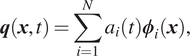 $$ \boldsymbol{q}\left(\boldsymbol{x},t\right)=\sum \limits_{i=1}^N{a}_i(t){\boldsymbol{\phi}}_i\left(\boldsymbol{x}\right), $$
where  $ N $ is the number of modes to be used. At most, $ N $ is equal to the dimension of the state vector, $ {N}_q $. To reduce the order of the model, only a subset of these modes can be kept, discarding the least energy/information carrying modes. Here, we use the method of snapshots to construct the POD modes from a database of the observations from which we will keep the $ M $ most energy-containing modes to construct a physics-based reduced order model of the system under study (Berkooz et al., Reference Berkooz, Holmes and Lumley1993). The method to obtain the POD is described hereunder.
Let  $ \boldsymbol{Q}\in {\unicode{x211D}}^{N_q\times {N}_t} $ be a matrix concatenating all the observations (snapshots), where $ {N}_t $ is the number of snapshots. From $ \boldsymbol{Q} $, the covariance matrix $ \boldsymbol{C} $ can be computed:
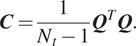 $$ \boldsymbol{C}=\frac{1}{N_t-1}{\boldsymbol{Q}}^T\boldsymbol{Q}. $$
In fluid mechanics,  $ \boldsymbol{q} $ usually is the velocity field and, therefore, half of the trace of $ \boldsymbol{C} $ is the turbulent kinetic energy and the eigenvalues of $ \boldsymbol{C} $ are a measure of the turbulent kinetic energy. The POD modes $ {\boldsymbol{\phi}}_i $ are then obtained by solving the eigenvalue problem:
 $$ \boldsymbol{C}{\boldsymbol{\phi}}_i={\lambda}_i{\boldsymbol{\phi}}_i. $$
The relative energy contribution of each POD mode can then be computed as  $ {\lambda}_i/{\sum}_i^N{\lambda}_i $ and the $ M $ most energy contributing modes can be considered in the reduced order model while the least energy containing ones are discarded.
Once the POD modes have been obtained, for example using singular value decomposition (SVD), their time-evolution can be deduced by projecting the original governing equations of the system under study onto a reduced base formed by a subset of the POD modes, following the Galerkin projection method (Matthies and Meyer, Reference Matthies and Meyer2003; Rowley et al., Reference Rowley, Colonius and Murray2004; Maulik et al., Reference Maulik, Lusch and Balaprakash2021). Let us consider a system governed by a generic PDE:
 $$ \dot{\boldsymbol{q}}\left(\boldsymbol{x},t\right)=\mathcal{N}\left[\boldsymbol{q}\left(\boldsymbol{x},t\right)\right]+\mathrm{\mathcal{L}}\left[\boldsymbol{q}\left(\boldsymbol{x},t\right)\right], $$
where  $ (\dot{\hskip0.333em }) $ is the time-derivative, $ \boldsymbol{x}\in \Omega $ is the spatial domain, $ t\in \left[0,T\right] $ is the time coordinate and where $ \mathcal{N} $ and $ \mathrm{\mathcal{L}} $ are nonlinear and linear operators, respectively. Using an appropriate spatial discretization, Equation (4) can be recast as a set of coupled ordinary differential equations (ODEs):
 $$ {\dot{\boldsymbol{q}}}_{\boldsymbol{h}}\left(\boldsymbol{x},t\right)={\mathcal{N}}_h\left[{\boldsymbol{q}}_{\boldsymbol{h}}\left(\boldsymbol{x},t\right)\right]+{\mathrm{\mathcal{L}}}_h\left[{\boldsymbol{q}}_{\boldsymbol{h}}\left(\boldsymbol{x},t\right)\right], $$
where  $ {\boldsymbol{q}}_{\boldsymbol{h}} $ is the full state vector expressed on the grid used to discretize the spatial dimension, and $ {\mathcal{N}}_h $ and $ {\mathrm{\mathcal{L}}}_h $ are the discretized version of the nonlinear and linear operators $ \mathcal{N} $ and $ \mathrm{\mathcal{L}} $, respectively, discretized on the considered grid. Using the POD-based basis (Equation (1)) which can be re-expressed as $ {\boldsymbol{q}}_h=\boldsymbol{\Phi} \boldsymbol{a} $, with $ \boldsymbol{\Phi} $ being the concatenation of all the POD modes, $ {\boldsymbol{\phi}}_i $, one can rewrite this as:
 $$ \boldsymbol{\Phi} \dot{\boldsymbol{a}}(t)={\mathcal{N}}_h\left[\boldsymbol{\Phi} \boldsymbol{a}(t)\right]+{\mathrm{\mathcal{L}}}_h\left[\boldsymbol{\Phi} \boldsymbol{a}(t)\right]. $$
Using the orthogonal nature of the POD decomposition (i.e., applying the inner product of Equation (6) with the POD mode  $ {\boldsymbol{\phi}}_k $ which are orthonormal to each other), the evolution equations for the modal amplitudes, $ \boldsymbol{a} $, can then be obtained:
 $$ \dot{\boldsymbol{a}}(t)={\boldsymbol{\Phi}}^T{\mathcal{N}}_h[\boldsymbol{\Phi} \boldsymbol{a}(t)]+{\mathcal{L}}_r[\boldsymbol{a}(t)]. $$
For each individual modal coefficient,  $ {a}_k $, the equation above with quadratic nonlinearities reads (Pawar et al., Reference Pawar, Ahmed, San and Rasheed2020; Maulik et al., Reference Maulik, Lusch and Balaprakash2021):
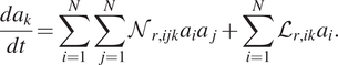 $$ \frac{d{a}_k}{dt}=\sum \limits_{i=1}^N\sum \limits_{j=1}^N{\mathcal{N}}_{r,ijk}{a}_i{a}_j+\sum \limits_{i=1}^N{\mathcal{L}}_{r,ik}{a}_i. $$
where  $ {\mathcal{N}}_{r,ijk} $ and $ {\mathcal{L}}_{r,ik} $ are the coefficients of the reduced discretized nonlinear and reduced linear operators, $ {\mathcal{N}}_r $ and $ {\mathcal{L}}_r $ respectively, in Equation (7). The set of ODEs in Equation (8) can then be simulated using traditional time-integration techniques such as a Runge–Kutta 4 technique for example.
Additional details on the POD/Galerkin projection approach can be found in Maulik et al. (Reference Maulik, Lusch and Balaprakash2021) and Pawar et al. (Reference Pawar, Ahmed, San and Rasheed2020) for the interested readers.
2.2. Echo state network
The ESN approach, shown in Figure 1a, presented by Lukoševičius (Reference Lukoševičius, Montavon, Orr and Muller2012) with the modification introduced by Pathak et al. (Reference Pathak, Wikner, Fussell, Chandra, Hunt, Girvan and Ott2018b) is used here. Given a training input signal  $ \boldsymbol{u}(n)\in {\unicode{x211D}}^{N_u} $ and a desired known target output signal $ \boldsymbol{y}(n)\in {\unicode{x211D}}^{N_y} $, the ESN learns a model with output $ \hat{\boldsymbol{y}}(n) $ matching $ \boldsymbol{y}(n) $. $ n=1,\dots, {N}_t $ is the number of time steps, and $ {N}_t $ is the number of data points in the training dataset covering a time window from $ 0 $ until $ T=\left({N}_t-1\right)\Delta t. $ Here, where the forecasting of a dynamical system is under investigation, the desired output signal is equal to the input signal at the next time step, that is, $ \boldsymbol{y}(n)=\boldsymbol{u}(n+1)\in {\mathbb{\mathrm{R}}}^{N_y={N}_u} $.
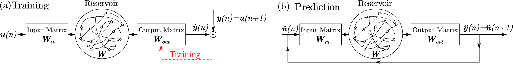
Figure 1. Schematic of the echo state network (ESN) during (a) training and (b) future prediction.
The ESN is composed of a randomized high-dimensional dynamical system, called a reservoir, whose states at time  $ n $ are represented by a vector, $ \boldsymbol{x}(n)\in {\unicode{x211D}}^{N_x} $ representing the reservoir neuron activations. The reservoir is coupled to the input signal, $ \boldsymbol{u} $, via an input-to-reservoir matrix, $ {\boldsymbol{W}}_{in}\in {\unicode{x211D}}^{N_x\times {N}_u} $. Following studies in Pathak et al. (Reference Pathak, Wikner, Fussell, Chandra, Hunt, Girvan and Ott2018b), before coupling the reservoir states to the output, a quadratic transformation is applied to the reservoir states:
 $$ {\tilde{x}}_i=\left\{\begin{array}{c}{x}_i,\hskip0.5em \mathrm{if}\hskip0.5em i\hskip0.5em \mathrm{odd},\\ {}{x}_i^2,\hskip0.5em \mathrm{if}\hskip0.5em i\hskip0.5em \mathrm{even}.\end{array}\right. $$
The output of the reservoir,  $ \hat{\boldsymbol{y}} $, is then deduced from these modified states via the reservoir-to-output matrix, $ {\boldsymbol{W}}_{out}\in {\unicode{x211D}}^{N_y\times {N}_x} $, as a linear combination of the modified reservoir states:
 $$ \hat{\boldsymbol{y}}={\boldsymbol{W}}_{out}\tilde{\boldsymbol{x}}. $$
In this work, a leaky reservoir is used, in which the state of the reservoir evolves according to:
 $$ {\boldsymbol{x}}^{+}\left(n+1\right)=\tanh \left({\boldsymbol{W}}_{in}\boldsymbol{u}\left(n+1\right)+\boldsymbol{Wx}(n)\right), $$
 $$ \boldsymbol{x}\left(n+1\right)=\left(1-\alpha \right)\boldsymbol{x}(n)+\alpha {\boldsymbol{x}}^{+}(n), $$
where  $ \boldsymbol{W}\in {\unicode{x211D}}^{N_x\times {N}_x} $ is the recurrent weight matrix and the (element-wise) $ \tanh $ function is used as an activation function for the reservoir neurons. $ \alpha \in \left(0,1\right] $ is the leaking rate. The $ \tanh $ activation function is used here as it is the most common activation used (Lukoševičius and Jaeger, Reference Lukoševičius and Jaeger2009; Lukoševičius, Reference Lukoševičius, Montavon, Orr and Muller2012) and because, when combined with the quadratic transformation (Equation (9)), can provide appropriate accuracy (Herteux and Räth, Reference Herteux and Räth2020).
In the conventional ESN approach (Figure 1a), the input and recurrent matrices,  $ {\boldsymbol{W}}_{in} $ and $ \boldsymbol{W}, $ are randomly initialized only once and are not trained. These are typically sparse matrices constructed so that the reservoir verifies the echo state property (Jaeger and Haas, Reference Jaeger and Haas2004). Only the output matrix, $ {\boldsymbol{W}}_{out} $, is trained to minimize the mean squared error, $ L $, between the ESN predictions and the data:
 $$ L=\frac{1}{N_y}\sum \limits_{i=1}^{N_y}\frac{1}{N_t}\sum \limits_{n=1}^{N_t}{\left({\hat{y}}_i(n)-{y}_i(n)\right)}^2. $$
Following Pathak et al. (Reference Pathak, Wikner, Fussell, Chandra, Hunt, Girvan and Ott2018b),  $ {\boldsymbol{W}}_{in} $ is generated for each row of the matrix to have only one randomly chosen nonzero element, which is independently taken from a uniform distribution in the interval $ \left[-{\sigma}_{\mathrm{in}},{\sigma}_{\mathrm{in}}\right] $. $ \boldsymbol{W} $ is constructed to have an average connectivity $ \left\langle d\right\rangle $ and the non-zero elements are taken from a uniform distribution over the interval $ \left[-1,1\right] $. All the coefficients of $ \boldsymbol{W} $ are then multiplied by a constant coefficient for the largest absolute eigenvalue of $ \boldsymbol{W} $ to be equal to a value $ \rho $. $ \rho $ is here chosen to be smaller than 1 as, in most situations, this ensures the echo state property (Lukoševičius and Jaeger, Reference Lukoševičius and Jaeger2009; Lukoševičius, Reference Lukoševičius, Montavon, Orr and Muller2012). It should be noted that it is possible to use values larger than 1 while not violating this echo state property and there exist cases where using a value smaller than 1 does not guarantee the echo state property (Yildiz et al., Reference Yildiz, Jaeger and Kiebel2012; Jiang and Lai, Reference Jiang and Lai2019).
The training of the ESN consists in the optimization of  $ {\boldsymbol{W}}_{out} $. As the outputs of the ESN, $ \hat{\boldsymbol{y}} $, are a linear combination of the modified states, $ \tilde{\boldsymbol{x}} $, $ {\boldsymbol{W}}_{out} $ can be obtained by using ridge regression:
 $$ {\boldsymbol{W}}_{out}={\boldsymbol{YX}}^T{\left({\boldsymbol{XX}}^T+\gamma \boldsymbol{I}\right)}^{-1}, $$
where  $ \boldsymbol{Y} $ and $ \boldsymbol{X} $ are respectively the column-concatenation of the various time instants of the output data, $ \boldsymbol{y} $, and associated modified ESN states $ \tilde{\boldsymbol{x}} $. $ \gamma $ is a Tikhonov regularization factor. The optimization in Equation (14) is:
 $$ {\boldsymbol{W}}_{out}=\underset{{\boldsymbol{W}}_{out}}{\mathrm{argmin}}\frac{1}{N_y}\sum \limits_{i=1}^{N_y}\left(\sum \limits_{n=1}^{N_t}{\left({\hat{y}}_i(n)-{y}_i(n)\right)}^2+\gamma {\left\Vert {\boldsymbol{w}}_{out,i}\right\Vert}^2\right), $$
where  $ {\boldsymbol{w}}_{out,i} $ denotes the $ i $th row of $ {\boldsymbol{W}}_{out} $ and $ \left\Vert \cdot \right\Vert $ is the $ L2 $-norm. This optimization problem penalizes large values of $ {\boldsymbol{W}}_{out} $, which generally improves the feedback stability and avoids overfitting (Lukoševičius, Reference Lukoševičius, Montavon, Orr and Muller2012).
After training, to obtain predictions for future times  $ t>T $, the output of the ESN is looped back as an input, which evolves autonomously (Figure 1b).
2.3. Hybrid approach in reduced-order space
The method presented here is inspired from Pawar et al. (Reference Pawar, Ahmed, San and Rasheed2020) and is shown in Figure 2. In a first step, the POD modes,  $ {\boldsymbol{\phi}}_k $, are obtained from the available training dataset with the method of snapshots by solving the eigenvalue problem (Eq. (3)). This eigenvalue problem is solved using SVD as in Pawar et al. (Reference Pawar, Ahmed, San and Rasheed2020), and the POD modes, $ {\boldsymbol{\phi}}_k $, are therefore obtained. Using a subset, $ M $, of these POD modes, the full system state, $ \boldsymbol{q} $, is then approximated as:
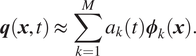 $$ \boldsymbol{q}\left(\boldsymbol{x},t\right)\approx \sum \limits_{k=1}^M{a}_k(t){\boldsymbol{\phi}}_k\left(\boldsymbol{x}\right). $$
Then, as described in Section 2.1, Galerkin projection is used to deduced the dynamics of the modal amplitude,  $ {a}_k $. Given that only a subset $ M $ of the POD modes are used, the governing equations for the modal amplitudes is slightly modified as:
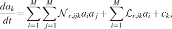 $$ \frac{d{a}_k}{dt}=\sum \limits_{i=1}^M\sum \limits_{j=1}^M{\mathcal{N}}_{r,ijk}{a}_i{a}_j+\sum \limits_{i=1}^M{\mathcal{L}}_{r,ik}{a}_i+{c}_k, $$
where  $ {c}_k $ is an error-term introduced that accounts for the effect of the truncated modes given that only $ M $ modes are used instead of all the POD modes. To simulate this set of ODEs, a combination of traditional time-integration and the ESN is then used: (a) the Equation (17) without the term $ {c}_k $ is time-advanced using traditional methods (such as the Runge–Kutta 4 scheme). This operation corresponds to the lower branch in Figure 2 where we obtain the approximation at the next time step, $ {\tilde{\boldsymbol{a}}}_{ROM}\left(n+1\right) $ from the modal amplitudes at the previous time-step, $ {\boldsymbol{a}}_{ROM}(n) $ and (b) the ESN is trained to learn the correction, $ \boldsymbol{c}\left(n+1\right) $, to add to the predicted modal coefficients estimated from time integration in (a) (the upper branch in Figure 2 where we estimate $ \boldsymbol{c}\left(n+1\right) $ from $ {\boldsymbol{a}}_{ROM}(n) $). Finally, from these corrected modal amplitudes, the prediction can then be reconstructed in physical space using the spatial modes, $ {\phi}_k $. Additional details on this architecture can be found in Pawar et al. (Reference Pawar, Ahmed, San and Rasheed2020).
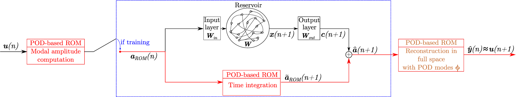
Figure 2. Architecture of the hybrid approach of Pawar et al. (Reference Pawar, Ahmed, San and Rasheed2020). The blue box indicates the actual hybrid architecture part.
It should be noted that because the reconstruction is always performed based on the modal coefficients in the reduced space, the achievable accuracy may be limited given that higher order modes are never used. In what follows, this approach will be called hybrid-ESN-A.
For future autonomous prediction, the predicted modal amplitude  $ \hat{\boldsymbol{a}}\left(n+1\right) $, is looped back as the input of the hybrid architecture and the system evolves autonomously (in modal space).
2.4. Hybrid approach in full space
Following an approach proposed in Pathak et al. (Reference Pathak, Wikner, Fussell, Chandra, Hunt, Girvan and Ott2018b), we investigate here the possibility of combining the ESN with a physics-based ROM obtained from POD-Galerkin projection to improve the overall accuracy. Compared to that earlier work, our approach may be more representative of what can actually be achieved in practical applications given that the physics-based model used by Pathak et al. (Reference Pathak, Wikner, Fussell, Chandra, Hunt, Girvan and Ott2018b) was just the original PDE governing the system with a small perturbation of one of the PDE parameters. Furthermore, using a POD-based ROM also allows to rigorously evaluate the impact of the accuracy of the physics-based model on the performance of the hybrid architecture by modifying the number of POD modes retained in the ROM. The architecture of this hybrid approach is shown in Figure 3.
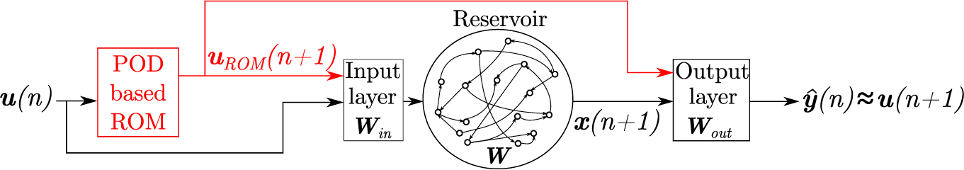
Figure 3. Architecture of the hybrid approach, inspired from Pathak et al. (Reference Pathak, Wikner, Fussell, Chandra, Hunt, Girvan and Ott2018b).
Here, the ROM is integrated to the conventional data-only ESN at two different streams (parts in red in Figure 3). On one the hand, the time-prediction of the ROM,  $ {\boldsymbol{u}}_{ROM}\left(n+1\right) $, is fed at the input of the ESN while at the same time, it is also provided at the output layer. This allows the reservoir to be influenced by the dynamics predicted by the ROM and for the ESN to make an appropriate blending at the output between the ROM prediction and its own reservoir states to provide an accurate prediction of $ \boldsymbol{u}\left(n+1\right) $. Therefore, the input to the ESN at time $ n $ is now:
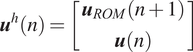 $$ {\boldsymbol{u}}^h(n)=\left[\begin{array}{c}{\boldsymbol{u}}_{ROM}\left(n+1\right)\\ {}\boldsymbol{u}(n)\end{array}\right] $$
and the output of the ESN is provided by the following equation:
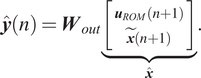 $$ \hat{\boldsymbol{y}}(n)={\boldsymbol{W}}_{out}\underset{\hat{\boldsymbol{x}}}{\underbrace{\left[\begin{array}{c}{\boldsymbol{u}}_{ROM}\left(n+1\right)\\ {}\tilde{\boldsymbol{x}}\left(n+1\right)\end{array}\right]}}. $$
This increase in the inputs to the ESN and at the output results in an increase in the size of the input and output matrices. Compared to the hybrid method described in the previous section, the ESN here is trained to learn the correction on the ROM prediction in the full space. In what follows, this approach will be noted hybrid-ESN-B.
To perform autonomous future prediction, the output of the architecture shown in Figure 3 is looped back at the input to make the hybrid-ESN-B able to evolve autonomously.
3. Results
The approaches described in Section 2 will be applied to learn the dynamics of two chaotic systems: the CDV system and the KS equation. For each of these systems, a reduced-order model will first be obtained by POD-Galerkin projection and a data-only ESN will be trained to learn their dynamics. Subsequently, the accuracy of these separate approaches will be compared to the hybrid approaches presented in Section 2.4.
3.1. CDV system
The CDV system is a chaotic low-order atmospheric model inspired by Crommelin et al. (Reference Crommelin, Opsteegh and Verhulst2004) that models the barotropic flow in a  $ \beta $-plane with orography. A truncated version of the CDV system is considered here and it is governed by the following set of ODEs (Crommelin et al., Reference Crommelin, Opsteegh and Verhulst2004; Crommelin and Majda, Reference Crommelin and Majda2004; Doan et al., Reference Doan, Polifke and Magri2020):
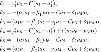 $$ {\displaystyle \begin{array}{l}{\dot{u}}_1={\gamma}_1^{\ast }{u}_3-C\left({u}_1-{u}_1^{\ast}\right),\\ {}{\dot{u}}_2=-\left({\alpha}_1{u}_1-{\beta}_1\right){u}_3-{Cu}_2-{\delta}_1{u}_4{u}_6,\\ {}{\dot{u}}_3=\left({\alpha}_1{u}_1-{\beta}_1\right){u}_2-{\gamma}_1{u}_1-{Cu}_3+{\delta}_1{u}_4{u}_5,\\ {}{\dot{u}}_4={\gamma}_2^{\ast }{u}_6-C\left({u}_4-{u}_4^{\ast}\right)+\varepsilon \left({u}_2{u}_6-{u}_3{u}_5\right),\\ {}{\dot{u}}_5=-\left({\alpha}_2{u}_1-{\beta}_2\right){u}_6-{Cu}_5-{\delta}_2{u}_4{u}_3.\\ {}{\dot{u}}_6=\left({\alpha}_2{u}_1-{\beta}_2\right){u}_5-{\gamma}_2{u}_4-{Cu}_6+{\delta}_2{u}_4{u}_2\end{array}} $$
This model was derived from the barotropic vorticity equation on a  $ \beta $-plane channel (Crommelin et al., Reference Crommelin, Opsteegh and Verhulst2004) using Galerkin projection to obtain the simplest model that combines the mechanisms of barotropic and topographic instabilities. This translates into a system that shows two distinct regimes: one characterized by a slow evolution (and a large decrease in $ {u}_1 $) and one with strong fluctuations of all modes. These correspond to “blocked” and “zonal” flow regimes, respectively, which originate from the combination of the barotropic and topographic instabilities (Crommelin et al., Reference Crommelin, Opsteegh and Verhulst2004): the transition from “zonal” to blocked is due to the barotropic instability while the topographic instability induces the transition from the “blocked” to “zonal” regimes. The definition and exact values of the parameters of the CDV system are provided in the Supplementary Materials and have been chosen so as to ensure a chaotic and intermittent behavior following Wan et al. (Reference Wan, Vlachas, Koumoutsakos and Sapsis2018). A detailed discussion of the effects of the model parameters on the dynamics of the CDV system is provided in Crommelin et al. (Reference Crommelin, Opsteegh and Verhulst2004).
The set of ODEs, Equation (20), is solved using a Runge–Kutta 4 method with a timestep of  $ \Delta t=0.1 $. A typical time evolution of the CDV system is shown in Figure 4 where the time is normalized using the largest Lyapunov exponent, $ {\lambda}_{\mathrm{max}} $. The largest Lyapunov exponent represent the exponential divergence rate of two system trajectories, which are initially infinitesimally close to each other (Strogatz, Reference Strogatz1994). Here, for the CDV system, $ {\lambda}_{\mathrm{max}}\approx 0.02 $.
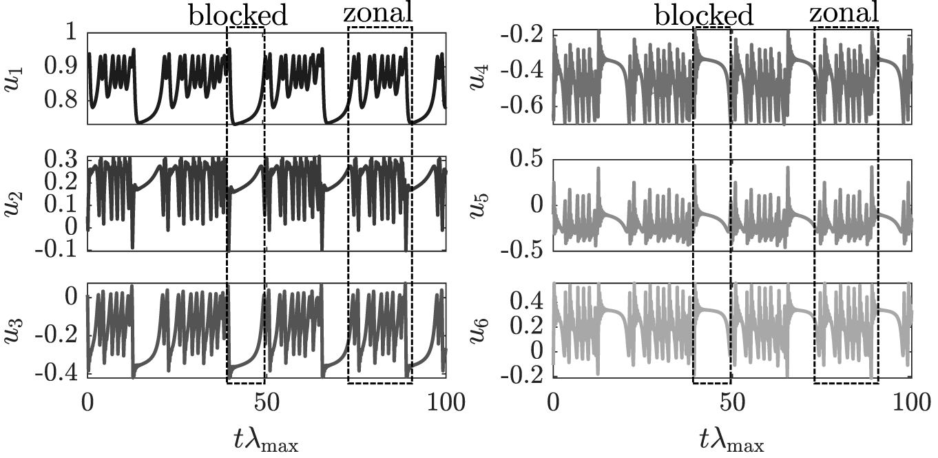
Figure 4. Time-evolution of the Charney–DeVore (CDV) system.
3.1.1. Reduced-order modeling of the CDV system
The POD method described in Section 2.1 is applied to the CDV system on a time-series that covers 100 Lyapunov time (with 62,500 snapshots). This corresponds to approximately four transitions from the blocked to zonal regime. This relatively short time-series is used to investigate the prediction capability of the proposed hybrid ROM/ESN approaches (to be discussed in Section 3.1.3) when a relatively small amount of data is available. The contributions of the eigenvalues obtained from the POD decomposition to the total energy of the CDV system is provided in Table 1. It can be seen that the vast majority of the energy is contained in the first three modes. However, discarding just one mode in the construction of the ROM for the CDV system already yields a very inaccurate model. Indeed, the time-prediction of the CDV model by a ROM composed of the first five POD modes is shown in Figure 5 where it is seen that it converges toward a fixed point after a small time during which it exhibits some dynamics. Therefore, for what follows, despite this inaccuracy, we will use this five POD-based ROM as the physics-based model in the hybrid approaches studied next as it is the most accurate nonperfect model achievable with POD and we will investigate whether adding an ESN can improve this accuracy.
Table 1. Relative energy contribution of each proper orthogonal decomposition (POD) modes to the total energy of the Charney–DeVore (CDV) system.
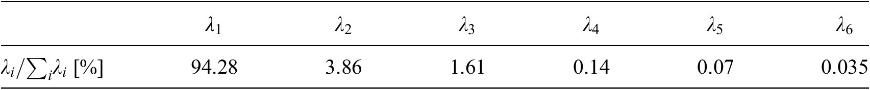
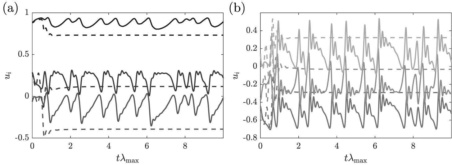
Figure 5. Time evolution of (a)  $ {u}_1 $– $ {u}_3 $ (dark to light gray) and (b) $ {u}_4 $– $ {u}_6 $ (dark to light gray) predicted by the proper orthogonal decomposition (POD)-based reduced order model (ROM; dashed lines) and of the full Charney–DeVore (CDV) system (full lines).
3.1.2. Data-only ESN
The standard data-only ESN (shown in Figure 1) is trained with the same dataset as the one used to develop the POD modes in Section 3.1.1. To estimate an adequate set of hyperparameters, following the guidelines by Lukoševičius (Reference Lukoševičius, Montavon, Orr and Muller2012), the reservoir size is first fixed to a size of 500 neurons. Thereafter, a series of line searches are performed for all hyperparameters to determine a locally optimal set of values for those hyperparameters. While more advanced hyperparameters search and accuracy assessment techniques exist (Lukoševičius and Uselis, Reference Lukoševičius and Uselis2019; Racca and Magri, Reference Racca and Magri2021), this approach is used here for its simplicity. Additional details on the procedure to determine the hyperparameters of the ESN, as well as the values used, are provided in the Supplementary Materials.
A time-prediction by a data-only ESN of 200 units is shown in Figure 6 where it can be seen that the ESN managed to learn the dynamics of the CDV system. Its accuracy is a marked improvement over the ROM shown in Figure 5 as the ESN prediction closely follows the actual CDV evolution for approximately 2.5 Lyapunov time (time multiplied by the largest Lyapunov exponent) and does not converge toward a fixed point. To quantify this prediction accuracy, similarly as in Pathak et al. (Reference Pathak, Wikner, Fussell, Chandra, Hunt, Girvan and Ott2018b), we define the prediction horizon,  $ {t}_{\mathrm{pred}} $, as the time it takes for the normalized error, $ \varepsilon $, to exceed 0.4, where $ \unicode{x03B5} $ is defined as:
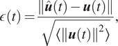 $$ \epsilon (t)=\frac{\left\Vert \hat{\boldsymbol{u}}(t)-\boldsymbol{u}(t)\right\Vert }{\sqrt{\left\langle {\left\Vert \boldsymbol{u}(t)\right\Vert}^2\right\rangle }}, $$
where  $ \left\Vert \cdot \right\Vert $ is the $ L2 $-norm and $ \left\langle \cdot \right\rangle $ indicates the time-average. $ \hat{\boldsymbol{u}} $ denotes the prediction from the ESN and $ \boldsymbol{u} $ the exact system evolution. This prediction horizon is indicated by the red line in Figure 6, with the time-evolution of $ \unicode{x03B5} $, shown in Figure 6c. This time-evolution of $ \unicode{x03B5} $ shows that the prediction from the ESN starts to deviate after 1 Lyapunov time but still remains close to the reference evolution for an additional 1.5 Lyapunov time.
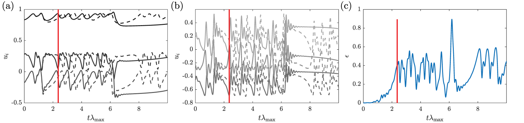
Figure 6. Time evolution of (a)  $ {u}_1 $– $ {u}_3 $ (dark to light gray), (b) $ {u}_4 $– $ {u}_6 $ (dark to light gray) predicted by the data-only echo state network (ESN) with 200 units (dashed lines) and of the full Charney–DeVore (CDV) system (full lines), and (c) associated time-evolution of the error between the predicted trajectory by the ESN and the reference trajectory. Red line indicates the prediction horizon.
To obtain a statistical estimate of the accuracy of the ESN, the trained ESN is tested in the following manner. First, the trained ESN is run for an ensemble of 100 different initial conditions. Second, for each run, the prediction horizon is calculated, as described above. Third, the mean and standard deviation of the prediction horizon are computed from the ensemble. This prediction horizon (expressed in normalized time) is shown in Figure 7 where it can be seen that, as the reservoir size increases, a better accuracy is achieved. However, the accuracy saturates at close to four Lyapunov times. This may be due to the limited dataset used for training which contains only a few transitiosn from blocked to zonal regimes. It is therefore possible that the ESN is not able to fully learn the dynamics of the CDV system.
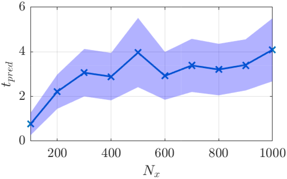
Figure 7. Prediction horizon of the data-only echo state network (ESN) for various reservoir sizes. Shaded area indicates one standard deviation around the mean of the prediction horizon.
3.1.3. Hybrid ESN prediction
The hybrid architectures, presented in Sections 2.3 and 2.4, that combine the POD/Galerkin-based ROM and an ESN are now studied. The hyperparameters of the ESN used in these hybrid architectures are obtained in a similar manner as for the data-only ESN and their values are reported in the Supplementary Materials. While the hyperparameter search method may have an impact on the comparative performance of the different considered architectures, given that the same search method is applied for all the considered architectures, the differences in performance should mainly originate from the difference in architecture.
The predictions by both hybrid architectures for the same initial condition as the one in Figure 6 are shown in Figure 8 where a reservoir of 200 neurons is also used. These predictions start to deviate from the reference evolution after a few Lyapunov times, as can be seen from the error evolution. However, the deviation remains moderate for a few additional Lyapunov times as the trajectory predicted by the hybrid approaches (especially hybrid-ESN-B), remains close to the reference one. However, after these additional Lyapunov times, the difference between the trajectories predicted by the hybrid approaches and the reference one increases further. This is to be expected given that these are chaotic systems and any small perturbation or inaccuracies will inevitably lead to two different trajectories (even if the dynamics of the chaotic system was perfectly learned by the hybrid approaches). Compared to the ROM-only and the data-only ESN, hybrid-ESN-A does not really show much improvement in accuracy while hybrid-ESN-B has a prediction horizon of approximately four Lyapunov times, compared to two for the data-only ESN. This latter improvement in accuracy shows that, despite having a fairly inaccurate ROM, the ROM can still contribute to an improvement in the accuracy of the ESN for hybrid-ESN-B. This is because the ESN only has to learn the correction on the ROM in full order space and not the complex dynamics of the full CDV system.
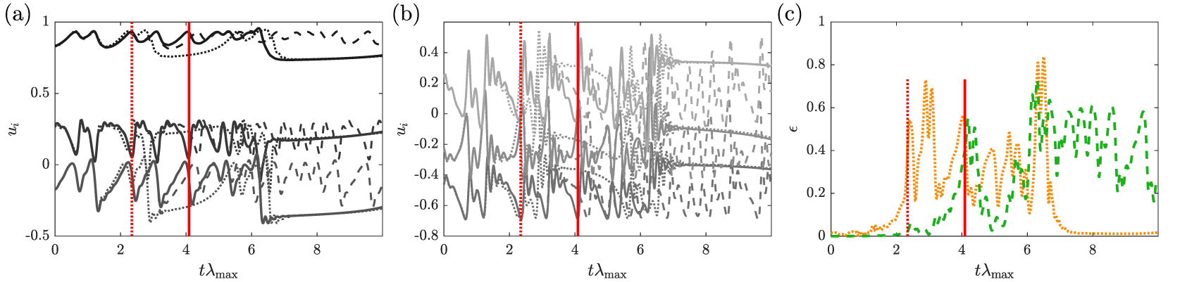
Figure 8. Time evolution of (a)  $ {u}_1 $– $ {u}_3 $ (dark to light gray), (b) $ {u}_4 $– $ {u}_6 $ (dark to light gray) predicted by the hybrid-echo state network (ESN)-A with 200 units (dotted lines), the hybrid-ESN-B with 200 units (dashed lines) and of the full Charney–DeVore (CDV) system (full lines), and (c) associated time-evolution of the error between the predicted trajectory by the hybrid-ESN-A (dotted line), by the hybrid-ESN-B (dashed line) and the reference trajectory. The red lines indicate the prediction horizon for the hybrid-ESN-A (dotted line) and hybrid-ESN-B (full line).
To further analyze the improvement obtained, the accuracy of the hybrid ESN approaches is assessed statistically, similarly to what was performed for the data-only ESN. This is shown in Figure 9 where the prediction horizons of the data-only ESN and of the POD-based ROM are also provided for comparison purposes. It can be seen that the prediction horizon of the hybrid-ESN-B is the largest for all reservoir sizes and it outperforms both the ROM-only and the data-only ESN with the largest improvement of two Lyapunov times obtained for a small reservoir size of 100 neurons. This highlights the beneficial effect on the accuracy of using a physics-based model in combination with the data-only approach, even with a model which has a flawed dynamics, here the convergence toward a fixed point. For larger reservoir sizes, the improvement over the data-only ESN is smaller but the hybrid ESN still outperforms the data-only ESN. It is also observed that the accuracy of the hybrid-ESN-B saturates for much smaller reservoir. This may originate from the fact that the dynamics that the ESN has to learn is more simple as, now, only the correction on the approximate ROM has to be learned.
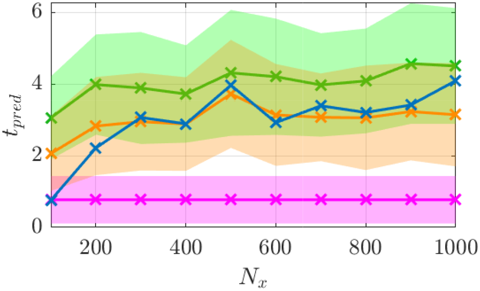
Figure 9. Prediction horizon for the Charney–DeVore (CDV) system of the reduced order model (ROM) only (magenta line and shaded area), the hybrid-echo state network (ESN)-A (orange dotted line and shaded area), the hybrid ESN-B (green line and shaded area), of the data-only ESN (blue line) for various reservoir sizes. Shaded area indicates the standard deviation of the prediction horizon. The standard deviation of the data-only ESN is shown in Figure 7.
On the other hand, the accuracy of the hybrid-ESN-A outperforms the data-only ESN for smaller reservoirs only (up to 200 neurons). After which, the accuracy of hybrid-ESN-A and the data-only ESN are similar. This could be explained by the fact that the reconstruction into the physical space is only performed using a reduced set of spatial modes which prevents a higher accuracy for hybrid-ESN-A.
Finally, as the prediction horizon may depend on the specific realization of the ESN used in the data-only or hybrid approaches (Haluszczynski and Räth, Reference Haluszczynski and Räth2019), the prediction horizons were also re-computed using 10 different realizations (i.e., when different random seeds are used to generate the matrices  $ {\boldsymbol{W}}_{\mathrm{in}} $ and $ \boldsymbol{W} $). These predictions horizons are shown in Section S3.1 of the Supplementary Materials and exhibits the same trends as those shown here. This highlights the robustness of these findings with respect to the ESN realization.
3.1.4. Poincaré and Lyapunov analysis of the ESN and hybrid approaches
An additional analysis is performed here to assess the ability of the ESN and hybrid-ESN approaches to reproduce the long-term dynamics of the CDV system and not just the short-term evolution. This is done by performing long-term prediction of the CDV system (for 100 Lyapunov time) for reservoirs of 200 units and these are plotted in a Poincaré map composed of the  $ \left({u}_1,{u}_4\right) $ components of the CDV system. In that phase space, the switch from a zonal to a blocked regime can be observed, the zonal mode corresponding to the bottom right region in Figure 10a (large values of $ {u}_1 $ combined with small values of $ {u}_4 $) while the blocked regime corresponds to the top-right corner (small values of $ {u}_1 $ with large values of $ {u}_4 $). Compared to the short-term predictions discussed in the previous section, it becomes clear that the hybrid-ESN-B approach is best able to reproduce the dynamics of the CDV system as its trajectory, shown in Figure 10d, is the closest to the exact one in Figure 10a. Indeed, by comparison, the data-only ESN converges toward a fixed point after some dynamics (as highlighted by the arrow in Figure 10b) while the hybrid-ESN-A develops into a periodic evolution given that its trajectory in the Poincaré map does not show a dense trajectory. This analysis was repeated by increasing the reservoir size of the ESN to 1,000 units (not shown here for brevity). When that larger reservoir was used, the data-only ESN managed to reproduce accurately the same phase trajectory as the exact system. However, the hybrid-ESN-A still is unable to reproduce the same phase trajectory and this may be because all predictions are made in the reduced space and therefore, it may not be possible for that architecture to reproduce fully the chaotic dynamics.

Figure 10. Trajectory in phase space of the  $ {u}_1 $ and $ {u}_4 $ modes of the Charney–DeVore (CDV) system from (a) exact data, and predicted by (b) the data-only echo state network (ESN), (c) hybrid-ESN-A, and (d) hybrid-ESN-B. The ESN has 200 units in all cases.
Finally, a further assessment of the capacity of the data-only ESN and hybrid approaches to learn the dynamics of the CDV system is to check whether they possess the same Lyapunov exponent as the original system (Pathak et al., Reference Pathak, Lu, Hunt, Girvan and Ott2017). Here, for simplicity’s sake, we focus only on the largest Lyapunov exponent which can be computed in the following manner for each approach: (a) a first autonomous “unperturbed” prediction,  $ {\boldsymbol{u}}^u(t) $, is computed with a given initial condition $ {\boldsymbol{u}}_0 $; (b) a second perturbed autonomous prediction, $ {\boldsymbol{u}}^p(t) $ is computed where the initial condition is slightly perturbed, that is using $ {\boldsymbol{u}}_0+\unicode{x03B5} $ with $ \unicode{x03B5} ={10}^{-6} $; (c) the difference between the two predictions, called the separation trajectory, is computed as $ \left\Vert \delta \boldsymbol{u}(t)\right\Vert \hskip0.5em =\hskip0.5em \left\Vert {\boldsymbol{u}}^u(t)-{\boldsymbol{u}}^p(t)\right\Vert $; and (d) the largest Lyapunov can be computed as the slope of the region where $ \log \left(\left\Vert \delta \boldsymbol{u}(t)\right\Vert \right) $ grows linearly. These separations trajectories are shown in Figure 11 where it can be seen that the linear part of all the separation trajectories show similar slopes (within 2% of each other) indicating that the largest Lyapunov exponent of all approaches is close to the reference one (black line). It should be noted that the particular shape of the separation trajectory of the hybrid-ESN-A approach (in red) is due to the periodic dynamics which is predicted by hybrid-ESN-A.
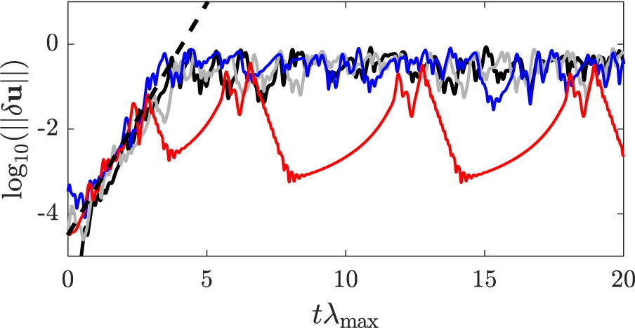
Figure 11. Separation trajectories of the reference system (black line), of the data-only echo state network (ESN; gray line), of the hybrid-ESN-A (red line) and of the hybrid-ESN-B (blue line). The ESN has 200 units in all cases. The dashed lines indicate the slope of the linear region of the separation trajectories.
3.2. KS equation
The KS system is a fourth-order nonlinear chaotic partial differential equation governed by Manneville (Reference Manneville, Frisch, Keller, Papanicolaou and Pironneau1985)
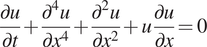 $$ \frac{\partial u}{\partial t}+\frac{\partial^4u}{\partial {x}^4}+\frac{\partial^2u}{\partial {x}^2}+u\frac{\partial u}{\partial x}=0 $$
defined over a domain  $ x\in \left[0,L\right] $ with periodic boundary conditions. The following initial condition is considered:
 $$ u\left(0,x\right)=\cos \left(2\pi \frac{x}{L}\right)\left[1+\sin \left(2\pi \frac{x}{L}\right)\right]. $$
The length  $ L $ plays a major role for the spatio-temporal chaos since the bifurcation parameter strongly depends on it: for small domain sizes, nonchaotic traveling waves emerge while, for larger domain sizes, intermittent bursts start to occur and disrupt the ordered structure resulting in a chaotic evolution (Manneville, Reference Manneville, Frisch, Keller, Papanicolaou and Pironneau1985).
In this work, we consider  $ L=35 $ to ensure this chaotic evolution and we solve Equation (22) using a spectral method with a Runge–Kutta 4 method for time advancement. The spatial domain is discretized using $ 64 $ grid points and a timestep
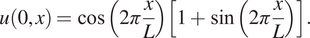
  $ \Delta t=0.25 $ is used. A typical spatio-temporal evolution of the KS system is shown in Figure 12 where the time is normalized using the largest Lyapunov exponent, $ {\lambda}_{max} $. For the KS equation, $ {\lambda}_{\mathrm{max}} $ is equal to 0.07. In what follows, similarly as for the CDV system, a dataset covering 100 Lyapunov time is used for the development of ROM and the training of the ESN is presented next.
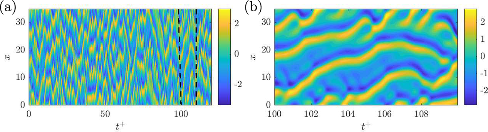
Figure 12. (a) Spatio-temporal evolution of the Kuramoto–Sivashinsky system and (b) zoom in the time between the black dashed lines in (a).  $ {t}^{+}={\lambda}_{\mathrm{max}}t $ is the normalized time.
3.2.1. Reduced-order modeling of the KS system
Similarly to what was done for the CDV system in Section 3.1.1, we apply the method of snapshots to obtain the POD modes of the KS system using a time series of 100 Lyapunov time which corresponds to 5,714 snapshots (the first 100 Lyapunov time shown in Figure 12a). The energy content of each mode is shown in Figure 13. It is observed that the first 19 modes contains most of the energy content of the KS system and these modes will be used for the ROM.
Figure 13. Relative energy content of each mode in the proper orthogonal decomposition (POD) decomposition of the Kuramoto–Sivashinsky (KS) system.
A typical time-evolution obtained from this ROM composed of 19 modes is shown in Figure 14a for the same time period as the one shown in Figure 12b. It can be seen that, compared to the actual evolution of the KS system (Figure 12b), this ROM does not manage to predict the dynamics of the KS system and seems to converge toward a fixed point after a small dynamics similar to what was observed for the ROM from the CDV system. The absolute error (shown in Figure 14c) shows that there is a rapid divergence between the ROM and the actual evolution with a large error already reached for less than one Lyapunov time. In comparison, Figure 14b,d shows the evolution and absolute error for a ROM constructed using 29 POD modes and it can be clearly seen that this larger ROM can accurately predict the evolution of the KS system for a longer time (approximately two Lyapunov time) but that the complex chaotic dynamics of the KS system is not fully capture either as the ROM seems to converge toward a quasi-periodic evolution.

Figure 14. Time-evolution of the proper orthogonal decomposition (POD)-based reduced order model (ROM) with (a) 19 modes and (b) 29 modes and (c and d) absolute error with respect to the full-order evolution.
3.2.2. Data-only ESN
Similarly to what was performed for the CDV system in Section 3.1.2, the ESN is trained using the same dataset as the one used to develop the POD modes. A similar optimization strategy as for the CDV system is used to obtain a set of adequate hyperparameters. The values of the hyperparameters for the data-only ESN are provided in the Supplementary Materials.
In a first stage, we assess here the ability of the ESN to learn the dynamics of the Kuramoto-Sivashinsky system. A singular prediction of the KS system is shown in Figure 15 for an ESN with a reservoir size of 500 units. In that figure, it can be seen that the ESN is able to qualitatively reproduce the dynamics of the KS system better than the ROMs of Section 3.2.1. Furthermore, the ESN is able to accurately predict the evolution of the KS system for approximately 1.5 Lyapunov time, indicated by the red line which represents the prediction horizon. After that, the trajectory predicted by the ESN diverges from the exact evolution.

Figure 15. (a) Prediction of the Kuramoto–Sivashinsky (KS) system by the data-only echo state network (ESN) with 500 units and (b) associated absolute error. The red line indicates the prediction horizon.
The statistical accuracy of the ESN for various reservoir sizes is shown in Figure 16 where it can be seen that, as the reservoir size increases, a longer prediction horizon is obtained before a saturation is observed. This latter saturation is likely due to the relative small dataset from which the ESN can learn the dynamics of the KS system.
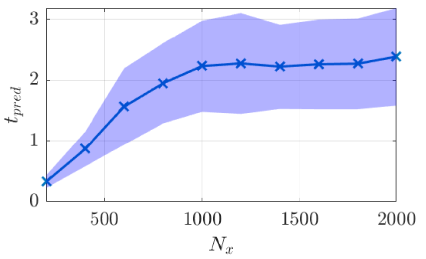
Figure 16. Prediction horizon of the data-only echo state network (ESN) for various reservoir sizes. Shaded area indicates the standard deviation of the prediction horizon.
3.2.3. Hybrid ESN prediction
We now analyze the predictions from the hybrid ESN approaches. The hyperparameters of the ESN for both hybrid architectures, obtained similarly as for the CDV case, are reported in the Supplementary Materials.
On one hand, we investigate what is the improvement provided by a given ESN for different levels of accuracy of the ROMs and, on the other hand, we explore whether for a given ROM, what is the level of improvement that can be obtained by including an ESN with reservoirs of different sizes to learn the dynamics of the KS system.
In Figure 17, predictions from hybrid-ESN-B are shown. For these, the hybrid-ESN-B has a fixed reservoir size of 500 neurons and two different ROMS are considered. In Figure 17a, a ROM of 19 modes is used and it can be seen that the accuracy is similar to the one of the ESN without ROM. This would indicate that the ROM with 19 modes is fairly inaccurate, as could be seen in Figure 14a, and that the hybrid-ESN-B is unable to use the ROM information in a meaningful manner to improve the accuracy of its prediction. When a ROM of 29 modes is used (Figure 17b), the accuracy of the hybrid ESN is much larger than with the ROM-only (Figure 14b) or the ESN without ROM (Figure 15b). The prediction horizon reaches approximately four Lyapunov times which is an improvement of two Lyapunov times compared to the ESN without ROM or the ROM only. It should be noted that, despite the prediction horizon being close to four Lyapunov times, the prediction from hybrid-ESN-B already shows some deviation from the reference trajectory starting from two Lyapunov times, as can be seen from the absolute error in Figure 15b. Nonetheless, similarly as for what was observed for the CDV system, this error remains bounded as the evolution predicted by hybrid-ESN-B remains close to the reference one (comparing Figure 17b with Figure 12b) for a longer period. After this, the error keeps increasing which is inevitable given that the KS system is a chaotic system.

Figure 17. Time-evolution of the hybrid-echo state network (ESN)-B with a reservoir of 500 neurons with a reduced order model (ROM) composed of (a) 19 modes, (b) 29 modes, and (c and d) absolute error with respect to the full-order evolution.
For hybrid-ESN-A, the predictions for a specific time instant are not shown for brevity and its accuracy is only assessed statistically in Figure 18 where it is analyzed for different reservoir sizes and ROM accuracy. In that figure, the accuracy of hybrid-ESN-B is also shown as well as the ones for the ROM and the standard ESN. For ROM of low accuracy with 19 modes (see Figure 18a), it can be seen that the accuracy of hybrid-ESN-A is smaller than the one from the data-only ESN, except for very small reservoir. This is due to the intrinsic limitation of the architecture that only uses the reduced number of spatial modes to reconstruct the full states. As a result, there are too few modes to enable an accurate reconstruction. In contrast, when a ROM with 29 modes is used (Figure 18b), the accuracy of hybrid-ESN-A is much larger. Additionally, for both ROMs, it is seen that the accuracy of hybrid-ESN-A does not increase much with the reservoir size indicating that the correction that the ESN can provide on the evolution of the retained modal coefficients is limited.
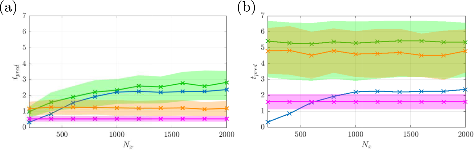
Figure 18. (a) With reduced order model (ROM) of 19 modes: prediction horizon of the ROM (magenta line and shaded area), of the hybrid-echo state network (ESN)-A (orange line and shaded area), of hybrid-ESN-B (green line and shaded area) for different reservoir sizes and of the data-only ESN (blue line). (b) With ROM of 29 modes: prediction horizon of the ROM (magenta line and shaded area), of the hybrid-ESN-A (orange line and shaded area), of hybrid-ESN-B (green line and shaded area) for different reservoir sizes and of the data-only ESN (blue line). Shaded areas indicate the standard deviation from the average prediction horizon. The standard deviation of the data-only ESN is shown in Figure 16.
For hybrid-ESN-B, when considering a ROM of 19 modes, it is seen that including this ROM with the ESN has a positive effect on the accuracy of the hybrid ESN (green curve compared to the blue one) which consistently outperforms the ESN without a ROM for all reservoir sizes. This improvement is marked the most clearly for small reservoir sizes. However, the improvement is more limited for larger reservoir sizes which is due to the fairly inaccurate ROM which has an average prediction horizon of only 0.5 Lyapunov time (magenta curve).
In contrast, when a ROM of 29 modes is used in the hybrid-ESN-B (green curve in Figure 18b), a significant increase in prediction horizon is obtained with a prediction horizon of more than five Lyapunov time. This constitutes an increase by more than three Lyapunov time compared to the ROM itself (magenta curve) and of between three and four Lyapunov time for the data-only ESN depending on the reservoir size. Additionally, it is observed that the prediction horizon of the hybrid-ESN does not change much with the reservoir size. This is due to the fact that the ESN only needs to learn the error between the ROM and the exact evolution. Given that the ROM with 29 modes is already relatively accurate, as seen in Figures 14b and 18b (magenta curve), a small reservoir is sufficient to capture that evolution accurately. Additionally, it is seen that hybrid-ESN-B always outperforms hybrid-ESN-A which is due to the fact that the ESN learns the correction in full space and not just in the reduced space. This allows the ESN in hybrid-ESN-B to better improve the accuracy which is particularly useful when the base model is fairly inaccurate as in Figure 18a.
Additionally, similarly to what was done for the CDV system, to assess the robustness of the computed prediction horizon with respect to the realization of the ESN, the prediction horizons were also re-computed using 10 different realizations. These predictions horizons are presented in Section S3.2 of the Supplementary Materials and similar results as the one shown here were observed.
To better assess the improvement that adding an ESN to a ROM can provide, the prediction horizon of the hybrid ESN for a reservoir of 500 neurons is assessed when the number of modes retained in the ROM is varied. Here, for simplicity, the hyperparameters are kept constant to the values used for the case with 29 modes retained. This is shown in Figure 19 where the average prediction horizon of both hybrid methods are compared to the one of the ROM. It is seen that adding the ESN of that size to the ROM always provide an improvement in prediction horizon even for this small reservoir. It is seen that for that specific reservoir size, the increase in accuracy is similar between hybrid-ESN-A and hybrid-ESN-B. However, as observed in Figure 18a, when larger reservoir sizes are used hybrid-ESN-B can provide an additional increase in accuracy whereas hybrid-ESN-A does not.

Figure 19. Prediction horizon with reduced order models (ROMs) of different accuracy for the hybrid-echo state network (ESN)-A with a reservoir of 500 units (orange), for the hybrid-ESN-B with a reservoir of 500 units (blue) and of the ROM only (magenta). Shaded area indicates the standard deviation.
An additional comment can be made by comparing the performance obtained here compared to the ones in previous works (Pathak et al., Reference Pathak, Hunt, Girvan, Lu and Ott2018a) that also studied the KS system. In Pathak et al. (Reference Pathak, Hunt, Girvan, Lu and Ott2018a), the high accuracy is obtained with a model-free approach which may be due to the use of a much longer training dataset than the one used here, combined with a more complex architecture where multiple ESNs are used in parallel with a large reservoir (of 5,000 units). In Pathak et al. (Reference Pathak, Wikner, Fussell, Chandra, Hunt, Girvan and Ott2018b), the high accuracy most likely mainly originates from the very accurate physics-based model used. This model actually consists of the exact governing equations of the KS system but where only one parameter is slightly perturbed. Therefore, the ESN in the hybrid architecture of Pathak et al. (Reference Pathak, Wikner, Fussell, Chandra, Hunt, Girvan and Ott2018b) only has to learn a much simpler dynamics (the small difference between the exact equation and the perturbed ones) and a high prediction horizon can therefore be achieved. In comparison, our approach relies on a more realistic physics-based model that capture the essential dynamics of the KS system (contained in a subset of the POD modes).
3.2.4. Poincaré analysis of the ESN and hybrid approaches
Similarly as for the CDV system, the ability of the ESN and of the hybrid approaches to reproduce the long-term dynamics of the KS system is assessed by performing a long-term prediction of the KS system for 100 Lyapunov times. The obtained predictions are then plotted in a phase space composed of the kinetic energy,  $ k $, and dissipation, $ D $, defined as:
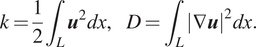 $$ k=\frac{1}{2}{\int}_L{\boldsymbol{u}}^2 dx,\hskip1em D={\int}_L{\left|\nabla \boldsymbol{u}\right|}^2 dx. $$
The trajectories in that phase space are shown in Figure 20 for reservoir sizes of 500 units, and 19 modes retained for the hybrid approaches. In that figure, it can be seen that the data-only ESN shows some inaccuracies in the prediction of the phase trajectories as it exhibits large excursion of  $ D $. On the other hand, both hybrid approaches are able to more accurately reproduce the trajectory of the KS system. However, when larger reservoir sizes are considered, the data-only ESN is able to more accurately reproduce the reference trajectory in phase space (not shown here for brevity). Similarly, for larger reservoirs or number of modes retained, the hybrid approaches are still able to reproduce the phase trajectory.
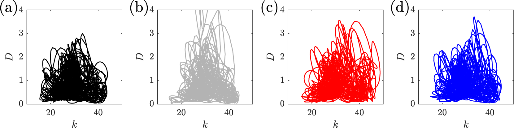
Figure 20. Trajectories in phase space of  $ k $ and $ D $ modes of the KS system from (a) exact data, and predicted by (b) the data-only echo state network (ESN), (c) the hybrid-ESN-A and (d) the hybrid-ESN-B. The ESN has 500 units in all cases and only 19 modes are retained for the hybrid approaches.
Finally, the largest Lyapunov exponent from the various approaches is also computed. The separation trajectories are shown in Figure 21, for reservoir sizes of 500 units and 19 modes retained, where it can be seen that all the approaches show a similar slope in their linear growth indicating that they all have similar largest Lyapunov exponent (within 5% of each other). This indicates that all the approaches can be used to approximate the largest Lyapunov exponent of this chaotic system. Similar results are obtained for larger reservoirs or more modes retained (not shown here for brevity).
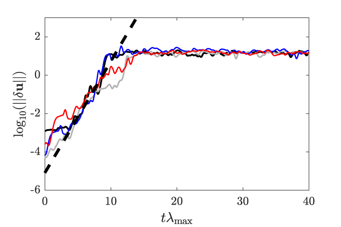
Figure 21. Separation trajectories of the reference system (black line), of the data-only echo state network (ESN; gray line), of the hybrid-ESN-A (red line) and of the hybrid-ESN-B (blue line). The ESN has 500 units in all cases and the hybrid approaches use 19 modes. The dashed lines indicate the slope of the linear region of the separation trajectories.
4. Discussion
For hybrid-ESN-B, it is seen from the architecture shown in Figure 3 that its prediction of the future system states comes from a combination of the predictions from the ROM and from the reservoir states. Therefore, an analysis of the weights in  $ {\boldsymbol{W}}_{out} $ can provide some insights into how the prediction is obtained from the reservoir states, $ \boldsymbol{x} $, and from the ROM prediction, $ {\boldsymbol{u}}_{ROM} $. To make such an analysis tractable, we compute the following term
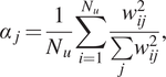 $$ {\alpha}_j=\frac{1}{N_u}\sum \limits_{i=1}^{N_u}\frac{w_{ij}^2}{\sum \limits_j{w}_{ij}^2}, $$
where  $ {w}_{ij} $ is the element at the $ i $th line, $ j $th column in $ {\boldsymbol{W}}_{out} $. The equation above provides the average normalized contribution of the $ j $th element in $ \hat{\boldsymbol{x}} $ to the $ i $th element of the prediction, $ {\hat{y}}_i $ (see Equation (19)). Therefore, if $ {\alpha}_i $ is large it means that that particular element from $ \hat{\boldsymbol{x}} $ has a significant contribution to the prediction $ \boldsymbol{y} $ (this can be a contribution to all elements of $ \boldsymbol{y} $ or a large contribution to a single element of $ \boldsymbol{y} $). Conversely, if $ {\alpha}_i $ is small, it indicates that that particular element in $ \hat{\boldsymbol{x}} $ does not contribute much to the prediction. In addition, let us recall that the first $ {N}_u $ elements in $ \hat{\boldsymbol{x}} $ come from the ROM prediction while the latter elements originate from the reservoir of the ESN. Therefore, this distinction between the two categories can provide an indication of the importance of the ROM-prediction and the respective reservoir states in the prediction of the future state. This calculation of $ {\alpha}_i $ is shown in Figure 22a for the cases with 19 and 29 modes retained in the ROM for a reservoir of 500 neurons. It is clearly seen that when an accurate ROM is used (with 29 retained modes, shown using the red curve), the most contributing elements of $ \hat{\boldsymbol{x}} $ are coming from the ROM as $ {\alpha}_i $ has large values for index 1–64 which corresponds to the ROM prediction while the $ {\alpha}_i $ for the subsequent elements are small. This was also observed for hybrid-ESN with larger reservoirs and this would explains why in Figure 18 little improvement is obtained in the prediction accuracy when a ROM of 29 modes for different reservoir sizes is used. The prediction mainly comes from the ROM and the reservoir of the ESN only needs to provide a small correction on that ROM prediction. Therefore a small reservoir is already sufficient to provide this correction.

Figure 22. (a) Relative contribution,  $ {\alpha}_i $, of the reduced order model (ROM) and reservoir states to the prediction for hybrid-echo state network (ESN) with ROM of 19 (green line) and 29 (red line) modes. (b) Overall contribution of the ROM, $ \Psi $, (blue line) and of the reservoir states, $ \Gamma $, (green line) to the overall hybrid-ESN with 500 units (full lines) and 2,000 units (dashed lines) for various ROM dimensions.
Conversely, when a more imprecise ROM with 19 retained modes is used (green curve), the opposite occurs. The contribution of the states coming from the ROM is much smaller than the one coming from the reservoir states and this means that, because the ROM is so imprecise, the ESN must mostly rely on its own reservoir states for the predictions. However, this does not mean that the ROM plays no role in the prediction as it will still influence the dynamics of the neurons in the reservoir and, as could be seen in Figure 18, an improvement in the prediction horizon can still be achieved.
This importance of the accuracy of the ROM can be further studied by analyzing the evolution of this weights repartition between ROM-prediction and reservoir prediction for different number of modes retained in the ROM and by splitting  $ {\alpha}_i $ into the 64 first terms (corresponding to the ROM) and the subsequent terms (corresponding to the reservoir state):
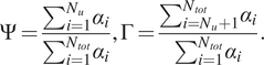 $$ \Psi =\frac{\sum_{i=1}^{N_u}{\alpha}_i}{\sum_{i=1}^{N_{tot}}{\alpha}_i},\Gamma =\frac{\sum_{i={N}_u+1}^{N_{tot}}{\alpha}_i}{\sum_{i=1}^{N_{tot}}{\alpha}_i}. $$ $ \Psi $ and $ \Gamma $ will give an indication of the overall weights of the ROM-based and reservoir states-based prediction, respectively. This is shown in Figure 22b where it has been computed for ROMs of various sizes and for two different reservoir sizes. Consistent with what was seen in Figure 22a, it can be seen that, for increasing modes retained in the ROM, the contributions from the reservoir states to the prediction decrease for both reservoir sizes considered. This is because the correction that the ESN has to provide decreases. It should be noted that, in that figure, to simplify the analysis and avoid having to perform a hyperparameter search for all ROM dimensions considered, the hyperparameters of the ESN are kept fixed for all ROM dimensions, using the value found for the case of hybrid-ESN-B with 19 modes. However, this analysis has also been repeated with the hyperparameters values used for the case of hybrid-ESN-B with 29 modes and the exact same trends as those shown in Figure 22 were also observed (not shown here for brevity).
5. Conclusion
In this work, we study two architectures that combine a reservoir computing approach, based on ESN, and a ROM obtained from POD/Galerkin projection. The first architecture, hybrid-ESN-A, is inspired by Pawar et al. (Reference Pawar, Ahmed, San and Rasheed2020) and is designed so that the ESN learns the correction of the modal amplitudes of the ROM and performs all predictions in the reduced-order space while the second architecture, hybrid-ESN-B, inspired by Pathak et al. (Reference Pathak, Wikner, Fussell, Chandra, Hunt, Girvan and Ott2018b), uses the prediction of the ROM in full space to excite the reservoir and makes a prediction based on the ROM prediction and the reservoir states. These architectures are used to learn and predict the chaotic dynamics of the CDV system and of the KS equation. The accuracy of these hybrid architectures is compared to the ROM only and to the standard ESN. It is seen that hybrid-ESN-B consistently predicts the exact evolution for a longer time than either the ROM or standard ESN while hybrid-ESN-A can only outperform the standard ESN for specific reservoir sizes. This latter could be due to the fact that hybrid-ESN-A performs all operation in the reduced space which inherently prevents a high accuracy. The effect of the accuracy of the ROM on the improvement in prediction is also rigorously assessed for the KS system by modifying the number of modes used in the ROM. It was seen that the accuracy of the ROM plays a crucial role in the improvement that can be obtained with an ESN. For a fairly inaccurate ROM, the improvement obtained with the hybrid-ESN-B, compared to the standard ESN, was fairly modest as the prediction from the ROM is too inaccurate for the hybrid-ESN-B architecture to use to predict accurately the evolution of the system. Conversely, when a more accurate ROM was used, a significant improvement was obtained and, in this case, a small reservoir was sufficient in the hybrid-ESN-B architecture for this improved accuracy. Additionally, it was observed that using a larger reservoir in combination with the accurate ROM did not yield increased accuracy. This is because the ESN part of the hybrid architecture only has to learn the correction to add on the ROM which may be much simpler to learn that the full system dynamics, especially if the ROM is already quite accurate. This effect of the accuracy of the ROM on the hybrid architecture is further studied by analyzing the weights in the output matrix in hybrid-ESN-B. On the one hand, it is found that when the ROM is inaccurate, its prediction is nearly not used by the hybrid-ESN-B architecture to predict the future evolution. Instead the prediction is constructed mostly from the reservoir states. On the other hand, when the ROM is accurate, the weights related to the ROM predictions are larger indicating that hybrid-ESN-B uses the ROM prediction to a large part in the prediction of the future state of the system.
In future work, these approaches will be applied to larger dimensional systems and on systems where the ROM is developed from physics-based consideration and not just from POD/Galerkin projection. The possibility of using the proposed approach with an LSTM will also be explored.
Supplementary Materials
To view supplementary material for this article, please visit http://dx.doi.org/10.1017/dce.2021.17.
Data Availability Statement
The data used for this research can be accessed upon reasonable request addressed to the authors.
Author Contributions
Conceptualization: N.A.K.D.; Data curation, Formal analysis, Investigation, Methodology, Validation, Visualization: M.L. and N.A.K.D.; Supervision: N.A.K.D.; Writing – original draft: M.L.; Writing – review & editing: N.A.K.D. and M.L. All authors approved the final submitted draft.
Funding Statement
Part of this research was supported by the Technical University of Munich - Institute for Advanced Study, funded by the German Excellence Initiative and the European Union Seventh Framework Program under grant agreement no. 291763.
Competing Interests
The authors declare no competing interests exist.


 Open access
Comments
No Comments have been published for this article.