


Policy Significance Statement
In this work, we develop a method to increase the amount of training data available to classify web-scraped price data. The need for large quantities of labeled data is a common theme across many machine learning (ML) methods and generating such data is time consuming and beyond the capabilities of many projects. Our method provides a way to expand a small number of labels to a large number with which a supervised ML method can be used. In future calculations of UK consumer price statistics, for which the method was developed, this will enable a much larger dataset to be leveraged which would not be possible if manual labeling alone was being considered.
1 Introduction
Research into alternative data sources for consumer price statistics is a key recommendation in the Johnson Review into UK consumer price statistics (Johnson, Reference Johnson2015), and the Independent Review of UK Economic Statistics (Bean, Reference Bean2016). Currently, the Office for National Statistics (ONS) produces the Consumer Prices Index including owner occupiers’ housing costs (CPIH) monthly from a basket of goods and services. Every month, the prices of products in the basket must be manually collected through a combination of sources, including price collectors visiting stores, collecting prices from websites and catalogues, and by phone.
Alternative data sources have the potential to improve the quality of these consumer price statistics through increased coverage, high frequency of collection, as well as potential cost savings. There is also potential to provide greater regional coverage of prices and expenditure such as, for example, regional inflation measures. There are two sources of alternative data that we are interested in: web-scraped data and point of sale transaction data. Both cover a much wider range of products and in much larger quantities than is possible with manual price collection. For example, we have recently started collecting web-scraped data for a number of items including clothing (ONS, 2018). In November 2018, the web-scraped data contained around 900,000 price quotes for clothing products. This compares to approximately 20,000 price quotes from the manual collection, a sample size increase of nearly 35 times.
However, while the manually collected data are much smaller in volume, each individual price quote is carefully checked and categorized into ONS’s item classifications (ONS, 2019a), an extension of COICOP5 (United Nations Statistics Division, 2018), by expert price collectors. The accuracy of the data is therefore very high and includes additional information which is not available to us in web-scraped data sources such as geographical location of the store from which the price is collected. Due to the sheer volume of web-scraped or scanner data that will be collected, it is impossible to manually classify every single product. Hence, we need to develop automated methods to classify the data to ONS item categories. These should be as accurate as possible to mitigate any reduction in classification accuracy while benefiting from the increased product coverage of the far larger data sets we expect from alternative data sources.
The sophistication of the methods required for automated classification varies greatly. For some items, this is relatively simple as there are well-defined rules that can be easily applied. For example, the current manual collection definition for laptops states that this category should not include refurbished products. A simple filter can remove these products by filtering on the word refurbished in the product name. However, some items, such as clothing, have complex collection definitions that rely on human judgment, that is what constitutes a fashion top? To replicate these judgments a more complex machine learning (ML) approach using features created from the text descriptions of products is required. We have a defined classification structure that lends itself to a supervised ML method. A supervised classifier attempts to learn rules to divide the data into provided categories (in this case, the ONS item categories). However, in order to learn how to perform the splitting, the algorithms need data that are already labeled into the desired categories. In most instances, we have only very limited labeled data points and it requires significant resource to create more. This gives us two challenges; how do we use text information in an ML classifier and how do we increase the number of labels so that we can train a supervised classifier without the need to manually label huge amounts of data?
This paper proposes an innovative new approach to these challenges using web-scraped clothing data as a pilot study. We apply methods similar to those used previously in ONS (2019a) to create numerical representations of text descriptions. We then make use of the semi-supervised ML techniques “label propagation” and “label spreading” to expand a small, representative number of labels to the rest of the dataset to train, test, and evaluate a number of supervised classifiers.
2 Background
It is important to understand this work in the context of the wider ONS project to transform consumer price statistics using new data sources and methods (ONS, 2019b). Accurate measures of inflation play a vital role in business, government, and everyday life. From rail fares to taxes to pensions, financial transactions in every area of our lives are regularly adjusted to reflect the change in prices over time. It is crucial to measure these changes in price as accurately as possible.
ONS is currently undergoing transformation across many areas of its statistics, including identifying new data sources and improving its methods. As part of this transformation, we are updating the way we collect price information to reflect our changing economy and produce more timely and granular inflation statistics for businesses, individuals, and government.
However, a significant period of research and analysis is required before these new sources can be fully integrated into headline estimates of consumer price indices, with an estimated completion date of Quarter 1 (January to March) 2023.
This research activity can be split into a number of workstreams. The classification workstream, to which this paper makes a significant contribution, looks at automatically classifying products to a specific item category. This work will recommend which methods are suitable for our prioritized item categories and for different data sources.
However, there are a number of other workstreams that will also need to be completed before these new sources can be integrated. For example, in the current methodology, the price for an individual product is followed over time and compared back to the price of the same product in the base period. An alternative approach would be to follow the average price of a defined group of homogeneous products instead. Research has shown this to be a viable alternative for categories such as clothing which experience high rates of product churn over time. Another work stream looks specifically at the web-scraped data: one of the limitations of these data is that it does not provide information on expenditure or quantities of product bought. This work will identify if the lack of expenditure weights at the product level introduces bias into any index based on web-scraped data, and if we can approximate expenditure weights using alternative data sources like page rankings. Other work streams are also in progress, focusing on aspects such as outlier detection, quality adjustment, and price index methodology. See ONS (2020) for the latest work program for alternative data sources including a full list of research work streams.
These workstreams will take place during 2020, in the research phase. This involves developing systems and methods (such as new methods of classification) for use with alternative data sources, alongside traditional sources and methods. The second phase, application, starts in 2021 and involves ONS applying these methods to specific categories such as clothing, groceries, and package holidays. This will include a full impact assessment and review of the implications of moving to using these new data sources and methods. Finally, in 2022, the third phase involves the release of quarterly experimental estimates of the impact of alternative data sources on consumer price statistics. Engagement with stakeholders and users about these changes will take place throughout the project.
3 Data
We have chosen to begin with web-scraped clothing data as it presents a particularly hard challenge. For many clothing categories, the collection definitions are ambiguous or hard to apply without the expert knowledge used by the price collectors to select the most suitable items. For example, deciding what constitutes a “fashion top” is subjective and requires human judgment. The collectors sometimes use features that are not included in the web-scraped data to establish if a product belongs to a category, such as if a shirt opens fully at the front, or what the sleeve length or neckline is. These uncertainties in the clothing category definitions make clothing hard to classify and methods developed here should apply to much of the rest of the CPIH basket.
For this pilot study, we are using a web-scraped dataset from World Global Style Network (WGSN).Footnote 1 Our data consist of daily prices and supplementary information from a number of fashion retailers’ websites. When this was supplied in 2015, the data contained content for 37 clothing product categories and 38 retailers in the United Kingdom, including a mixture of high street and online only retailers. The web-scraped data includes price, product, and retailer information. Women’s clothing data were provided for the period September 2013 to October 2015 and the men’s clothing data were provided for the period August 2014 to October 2015. The dataset is complex containing 67 ONS item categories in one dataset alongside some clothing that would not be included, such as girl’s dresses or women’s socks, and some nonclothing items retailers chose to include in the clothing sections such as gift cards, perfume or shoes.
This dataset therefore represents a multi-class classification problem where a product can belong to one of several categories. In this development phase, we use a small number out of all possible clothing categories to test the method (see Table 1). This includes an “other” category which contains a range of products that fall outside of the chosen categories. For example, perfume, vases, toys, and any clothing items not falling into one of the nine categories. The nine categories have been chosen as a small amount of labeled data that were already available for these categories to inform the classification process (ONS, 2017a; 2017b) Using these categories, we construct two sub samples of the full dataset to test and develop this approach. Each subsample contains 3,485 entries to mimic two months’ worth of data. This effectively provides a training and parameter optimization set and a second month as the out-of-sample test set to evaluate the method’s generalizability.
Table 1. Categories used in the clothing data with the number of each category present in the sample

4 Methods
Another feature of the WGSN data (which is also a challenge with web-scraped data more generally) is that it tends to combine data from several websites for the same category. As each website has a different layout, structure, and information about products, there are differences in the features and completeness from product to product. For example, some features are unavailable from certain retailers.
As the website information is intended for human audience, many of the attributes associated with a product are long text product names and descriptions. These require significant preprocessing before they can be used in the classification process. Due to the complex and diverse nature of the web-scraped data, we are required to employ several different methods in combination to expand the labeled dataset, create features, and perform classification. Below we will describe the methods used, these fall into four major categories: natural language processing (NLP), increasing the amount of labeled data, classification methods, and assessment metrics. Within each of these categories, we will discuss the methods appropriate for our use case.
4.1 Word embeddings
Creating numerical features from text data is a complex task with many different algorithms having been developed. These range from basic word counts to complex neural network based methods that attempt to capture context. In this work, as with the label matching (section “Term frequency—inverse document frequency”), we have used several methods and will combine the results of all three.
4.1.1 Count vectorization
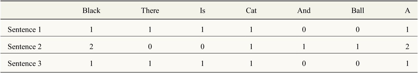
Count vectorization is one of the simplest ways to encode text information into a numerical representation first introduced by Jones (Reference Jones1972). Here, the number of times every word in the total corpus is found in a given sentence or phrase is used as the vector. For example, if we take the phrases:
Sentence 1: There is a black cat
Sentence 2: A black cat and a black ball
Sentence 3: Is there a black cat?
This results in the vectors shown in Table 2. These vectors have encoded the information contained in the sentences, however, this method offers no context for the words and different sentences can have the same representation as there is no encoding of word order. The above example demonstrates this as the first and last sentence have the same words (and therefore the same vectors) but different meaning.
Table 2. Demonstration of simple word vectorization method, count vectorization
One way to try and mitigate this is to use several words together, these are known as bi-grams for two words and tri-grams for three words. This leads to much larger vectors where pairs of words are considered in addition to single words. If we considered the bi-grams for the example in Table 2, we would no longer have the same vectors as “There is” and “is there” are different b-igrams. Therefore, we can distinguish between two sentences containing the same words, but with a different word order. In this work, we make use of bi-grams in addition to single words when calculation the word vectors.
This simple word vectorization method gives a baseline method for the word vectorization. They are conceptually simple to build, but there is a significant drawback when applying count vectorization model to new sentences. If the new sentences contain words not previously seen when building the model, they cannot be encoded.
4.1.2 Term frequency—inverse document frequency
Term frequency—inverse document frequency (TF-IDF) builds on the count vectorization method. It is a more sophisticated method of building the vectors as it attempts to give more prominence to more important words. TF-IDF does this by introducing a weighting to the words based on how commonly they appear in the total document. The logic of this is that the most frequently used words such as “the” and “a” will occur very often in a sentence, but they are not important for distinguishing the meaning of text in a document. Those less common but potentially more important words will be upweighted by the inverse document frequency defined below.
In this work, we use the Scikit-Learn implementation of the TF-IDF (Pedregosa et al., Reference Pedregosa, Varoquaux, Gramfort, Michel, Thirion, Grisel, Blondel, Prettenhofer, Weiss, Dubourg, Vanderplas, Passos, Cournapeau, Brucher, Perrot and Duchesnay2011). In this implementation, the term frequency is taken to be the count vectorization described in the previous section. The IDF is given by:
 $$ idf(t)=\log \frac{n_d}{df\left(d,t\right)}+1, $$
where the  $ {n}_d $
is the total number of documents/sentences and df(d,t) is the document frequency.
$ {n}_d $
is the total number of documents/sentences and df(d,t) is the document frequency.
Like the count vectorizer, however, it still does not account for the context of the words and cannot deal with new words that have not appeared before in previous documents. As with the count vectorizer, by extending the vectors to using bi- or tri-grams in addition to the single words, it is possible to allow for some context for the words, but this is limited. In this work, we make use of bi-grams in addition to the single words when training the TF-IDF vectors.
In Figure 1, we show a two-dimensional projection of the TF-IDF vectors for our dataset. These vectors have been projected using t-distributed stochastic neighbor embedding (t-SNE) algorithm that is well suited to visualizing high-dimensionality data in two or three dimensions (van der Maaten and Hinton, Reference van der and Hinton2008). Of course, with any reduction in dimensions, there is information lost along the way. This method attempts to preserve distances between the points, but not necessarily their higher dimensional structure, allowing us to identify clusters of points. We see in Figure 1 that some clothing items are better separated and more clustered in vector space than others. For example, shorts (yellow) and jeans (pale blue) are reasonably well separated. However, shirts (green) and top (dark orange) show much more overlap which makes sense given many of the same words would be used to describe these clothing items.

Figure 1. Two-dimensional projection of the word vector for a sample of clothing items generated using the term frequency—inverse document frequency algorithm.
4.1.3 word2vec
A more complex way to create numerical features from text is the word2vec algorithm (Mikolov et al., Reference Mikolov, Chen, Corrado and Dean2013). This method makes use of a shallow two-layer neural network to convert the words to word embeddings in a high-dimensional vector space. Word2vec works by creating a model to predict the next word given a target word and the surrounding context words of the rest of the document. For example, for the sentence “The mouse eats cheese from the box” if the target word was “eats,” the model would be attempting to predict “cheese” given the rest of the words in the sentence. The weights of the final hidden layer in this neural network are then taken as the word vectors to represent words of all the input sentences also known as the training corpus. A text corpus is a collection of structured written texts. The resulting word vectors for words which are similar will have similar vectors and so will occupy a similar area of the vector space in which they have been embedded. This means that unlike the count vectorization and the TF-IDF method, the context in which words are found is taken into consideration when generating the vectors. This is because the neural network was trained to predict the next word given the surrounding words so must consider context.
For this application, the words that we wish to embed are the product names, usually short phrases of typically 4–8 words. To obtain a single word vector for the product, we average the word vectors, obtained from each word in our sentence (e.g., a product name) together. This provides a single averaged vector for each product. The resulting word2vec vectors for our clothing dataset are shown in Figure 2. The word vectors here are showing several distinct clusters for the different clothing items with less overlap than was seen for the TF-IDF vectors.

Figure 2. Two-dimensional projection of the word vector for a sample of clothing items generated using the word2vec algorithm.
4.1.4 fastText
fastText is an algorithm that is built on very similar principles to word2vec (Bojanowski et al., Reference Bojanowski, Grave, Joulin and Mikolov2016). One of the major differences between the two algorithms is that the fastText algorithm uses character n-grams as well as whole words when constructing the predictive model. n-grams are substrings of a word of length n. For example, for the word “apple,” the bi-grams are ap, pp, pl, le, and the algorithm uses “ $ \Big\langle $
apple
$ \Big\langle $
apple $ \Big\rangle $
” to contain the whole word to prevent confusion between a whole word and a substring which is also a legitimate word.
$ \Big\rangle $
” to contain the whole word to prevent confusion between a whole word and a substring which is also a legitimate word.
By using the n-grams in addition to the whole words, the resulting word embeddings are better for rare words and are also able to cope with out-of-corpus words. This gives an advantage over the alternative word embedding techniques described previously as they are not able to handle out-of-corpus words. If an out-of-corpus word is encountered but the n-grams that make it up are available in the training data, a vector is constructed out of the n-gram vectors. A disadvantage of the fastText and word2vec methods are that they are complex to train. This could be mitigated by using pretrained vectors, but these would not be specialized for the use case of our data. For both the word2vec and fastText vectors, we make use of the gensim python library (Rehurek and Sojka, Reference Rehurek and Sojka2010) to train our word vector models on the clothing product names. The resulting fastText vectors for the clothing dataset are shown in Figure 3. In this projection, the vectors show significant clustering of different clothing types in different areas of vector space.

Figure 3. Two-dimensional projection of the word vector for a sample of clothing items generated using the fasttext algorithm.
4.2 Label propagation for increasing the amount of labeled data
Supervised ML methods require a large amount of accurately labeled data to train the algorithms to ensure that the classifiers are generalizable and able to better cope with new products. However, obtaining data that have already been labeled to the required ONS item level categorization of the CPIH basket is not possible and the task of manually labeling a large amount of data is an onerous one. Getting a limited number of labeled data points is often a more feasible option. It is then possible to expand the amount of labeled points available using the methods described below to generate a larger set of labels for training.
4.2.1 Fuzzy matching
We start the labeling process with a small number of manually produced labels, typically between 10 and 20 per ONS item category in our data. The initial labeled data are approximately 4% of the total dataset. We use string matching methods to provide a first-pass method to increase the number of products that have labels. These methods will assign labels to only those products that have a similar product name to those original labels. The first of these is the Levenshtein distance. This counts the minimum number of changes (inserting, changing, or deleting a character) required to turn one string into another. The second is the partial ratio method, which takes all substrings of the longer text that are of the same length of the shorter and returns the best match. This method is better at comparing strings of different lengths. For instance, blue stripy jumper and stripy jumper would be an exact match for the partial ratio (a value of 1) whereas they would have a Levenshtein distance of five as Levenshtein requires five-character insertions to match the strings “blue.” The third metric we use is the Jaccard distance. This takes all the characters in both strings as two sets and calculates the distance as follows:
 $$ 1-\frac{\mathrm{Length}\kern0.17em \mathrm{of}\kern0.17em \mathrm{the}\kern0.17em \mathrm{intersection}\kern0.17em \mathrm{of}\kern0.17em \mathrm{both}\kern0.17em \mathrm{strings}}{\mathrm{Length}\kern0.17em \mathrm{of}\kern0.17em \mathrm{the}\kern0.17em \mathrm{union}\kern0.17em \mathrm{of}\kern0.17em \mathrm{both}\ \mathrm{strings}}. $$
For the jumper example, the Jaccard distance is  $ 0.15 $
. A perfect match would be
$ 0.15 $
. A perfect match would be  $ 0 $
as the intersection and union of the strings would have the same length.
$ 0 $
as the intersection and union of the strings would have the same length.
Each of these metrics measure slightly different things and therefore have different advantages. It is hard to say which metric would give a definitive match. The Levenshtein distance is not well suited to strings of different length as each difference in length will be counted as a change even if the substrings match. For our use case, it is likely that the string lengths will vary quite substantially and so the Levenshtein distance will provide conservative matches. By contrast, the partial ratio technique will create matches for any product with the same substrings. This may provide more matches, but these will generally be of lower quality as just because the substring is an exact match the surrounding context words may mean it is not in reality a match within our classification hierarchy. The Jaccard distance also does not deal well with strings of different length as the extra length will increase the value in the denominator, resulting in lower scores where one string is a complete substring of another. This again will provide conservative matches. This method does though have a potential advantage in that it does not preserve character order, so a black hat and hat black would be a match. The sets used to calculate the intersection and union do not consider character order. This is desirable behavior for some strings and not for others. Due to these trade-offs between the metrics, we use all three metrics together and only accept a match if two out of the three distance metrics agree. This increases the precision of the fuzzy matched labels from around 70–90%, while only reducing the number of products labeled by 10%. As this approach will be used as the seed labels for the next step, this is a conservative method of finding matches as we want to minimize the false positives and improve the precision. In effect, what this approach does is find unlabeled products with very similar product names to the products in our labeled dataset, and assigns the unlabeled product that same label.
Future work may include an application of Named Entity Recognition techniques, which aim to identify the “target” of the next (the object at the heart of the description) before applying these techniques as this may facilitate a type of cleaning of the name fields prior to attempting to classify it.
4.2.2 Label propagation
Label propagation is part of a group of semi-supervised ML algorithms. Given our limited pool of labeled data points, semi-supervised learning can use these known labels in the learning process to steer an unsupervised learning approach to label the rest of the data, hence semi-supervised. In this work, we make use of the label propagation and label spreading algorithms from the scikit-learn python library (Pedregosa et al., Reference Pedregosa, Varoquaux, Gramfort, Michel, Thirion, Grisel, Blondel, Prettenhofer, Weiss, Dubourg, Vanderplas, Passos, Cournapeau, Brucher, Perrot and Duchesnay2011). These algorithms were introduced by Zhu and Ghahramani (Reference Zhu and Ghahramani2002) and Zhou et al. (Reference Zhou, Bousquet, Navin Lal, Weston and Sch Olkopf2004) and work in very similar ways. Both are graph (or network) based methods and make the essential assumption that data points that are close in the graph to a labeled point will likely share the same label.
In Figure 4, we illustrate what is meant by a graph in this context. The graph is a collection of points or nodes in some n-dimensional space that are connected via edges or links. These edges can either connect all nodes to all other nodes or can only connect to some. The left-hand panel of Figure 4 shows a two-dimensional example graph where each node is connected to its three nearest neighbors.

Figure 4. Illustration of the principles of the label propagation algorithm. The left-hand panel shows before the propagation algorithm, including the seed labels and the graph. The right-hand panel shows the result of running the label propagation algorithm correctly labeling the two clusters.
The graphs are not limited to two dimensions and can be constructed across the entire n-dimensional feature space. The graph is critical to the label propagation process and is most commonly produced using the K Nearest Neighbor (kNN) algorithm.Footnote 2 The principle of the kNN algorithm is to join each point to its K nearest neighbors where  $ k $
is an integer value. In the example in Figure 4, we have created the graph with a value of
$ k $
is an integer value. In the example in Figure 4, we have created the graph with a value of  $ k=3 $
. If k is equal to the number of points, this would be described as a fully connected graph.
$ k=3 $
. If k is equal to the number of points, this would be described as a fully connected graph.
The process of creating the graph is computationally intensive as each point must calculate the distance to each of the rest of the points in order to establish which are the k nearest. This will limit the use of this algorithm in extremely large datasets. In this work, we use Euclidean distance when calculating the graph; however, other metrics may be applied instead.
Once the graph is created the label propagation or spreading is then performed to “push” labeled points through the graph and so grow the labeled dataset. This is shown in Figure 4. In the left-hand panel, the graph and the seed labels are shown and in the right-hand panel, the result of the label propagation algorithm is shown. This shows that the red label has been propagated to the cluster nearest to it in the graph and similarly for the green.
The label propagation algorithm can be described in the following steps:
First, a probabilistic transition matrix T is defined, this is the distance between points weighted, so that close nodes are given more weight and further away nodes less and is given by:
 $$ {T}_{ij}=P\left(j\to i\right)=\frac{w_{ij}}{\sum_{k=1}^{l+u}{w}_{kj}}. $$
where  $ {T}_{ij} $
is the probability of a label jumping from node
$ {T}_{ij} $
is the probability of a label jumping from node  $ i $
to
$ i $
to  $ j $
and
$ j $
and  $ {w}_{ij} $
is the distance between the node
$ {w}_{ij} $
is the distance between the node  $ i $
and
$ i $
and  $ j $
normalized by the sum of the distance between all points. Here
$ j $
normalized by the sum of the distance between all points. Here  $ l $
is the number of labeled data points and
$ l $
is the number of labeled data points and  $ u $
is the number of unlabeled, this means that their sum is the total number of points in consideration. The remaining component of the initial set up is the labels of all points. For the labeled points, these will be defined already and the unlabeled points are assigned a dummy label of −1. This vector of label probabilities is given as
$ u $
is the number of unlabeled, this means that their sum is the total number of points in consideration. The remaining component of the initial set up is the labels of all points. For the labeled points, these will be defined already and the unlabeled points are assigned a dummy label of −1. This vector of label probabilities is given as  $ Y $
. The new labels of Y are then given by
$ Y $
. The new labels of Y are then given by
 $$ Y\leftarrow TY. $$
The  $ Y $
vectors are then renormalized, and the final step is to “clamp” the original labels back to be the same as the initial labeled points. This ensures that these known labels do not get changed during the label propagation process. It can be shown that this algorithm will iterate to convergence. For details, see Zhou et al. (Reference Zhou, Bousquet, Navin Lal, Weston and Sch Olkopf2004) or Bonoccorso (Reference Bonoccorso2018). The label propagation algorithm is similar to a Markov random walk and so shares properties with a Markov chain.
$ Y $
vectors are then renormalized, and the final step is to “clamp” the original labels back to be the same as the initial labeled points. This ensures that these known labels do not get changed during the label propagation process. It can be shown that this algorithm will iterate to convergence. For details, see Zhou et al. (Reference Zhou, Bousquet, Navin Lal, Weston and Sch Olkopf2004) or Bonoccorso (Reference Bonoccorso2018). The label propagation algorithm is similar to a Markov random walk and so shares properties with a Markov chain.
The other algorithm used in this work is label spreading. The basic idea of this algorithm is the same as that outlined above for label propagation except that the initial labels are not firmly clamped. Instead, some proportion of the labels are allowed to change. This is particularly helpful if the input labels are likely to be noisy and contain inaccurate examples, which is the case for our data as we have applied the fuzzy matching step to expand our initial labeled set. Here, the new labels are given by
 $$ {\tilde{Y}}^{t+1}=\alpha L{\tilde{Y}}^t+\left(1-\alpha \right){Y}^0, $$
where  $ t $
denotes the iteration,
$ t $
denotes the iteration,  $ {Y}^0 $
indicates the initial label probabilities, and
$ {Y}^0 $
indicates the initial label probabilities, and  $ \alpha $
is a number between 0 and 1. This enables a proportion of the initial labels to change. Similar to the label propagation method above, it can be proven that this algorithm does converge. For further details on the mathematics and graph theory behind this algorithm, see Zhu and Ghahramani (Reference Zhu and Ghahramani2002) and Bonoccorso (Reference Bonoccorso2018). We use the label spreading variant of label propagation here as the initial labels are noisy and not well defined for this dataset. This is because we have applied the first fuzzy matching step that expands the number of labeled products but introduces noise into the labels. As both the label propagation methods give a probability values for the new labels, we are able to choose what threshold of acceptance we want to use. By default in a binary classifier this would be 0.5 bu in this work we choose to use 0.7 as we want higher precision labels for the classifier. The newly labeled datasets can then be used to train a classifier, whether that is a ML method or simple filtering.
$ \alpha $
is a number between 0 and 1. This enables a proportion of the initial labels to change. Similar to the label propagation method above, it can be proven that this algorithm does converge. For further details on the mathematics and graph theory behind this algorithm, see Zhu and Ghahramani (Reference Zhu and Ghahramani2002) and Bonoccorso (Reference Bonoccorso2018). We use the label spreading variant of label propagation here as the initial labels are noisy and not well defined for this dataset. This is because we have applied the first fuzzy matching step that expands the number of labeled products but introduces noise into the labels. As both the label propagation methods give a probability values for the new labels, we are able to choose what threshold of acceptance we want to use. By default in a binary classifier this would be 0.5 bu in this work we choose to use 0.7 as we want higher precision labels for the classifier. The newly labeled datasets can then be used to train a classifier, whether that is a ML method or simple filtering.
4.3 Classification method
There are many different algorithms that have been developed to perform classification tasks. Not all algorithms are suitable for all datasets or problems and have varying levels of complexity and transparency. Below, we discuss the methods that are considered in this work.
4.3.1 Decision tree
A decision tree is an easy to interpret form of ML classifier. It can conceptually be thought of as a flowchart. The tree is built up of branches and nodes. At each node, a decision rule will split the data in two and this will then continue to the next node and the next. This process of splitting continues until a leaf is reached. Each leaf node is the target category being classified.
The decision tree is a supervised ML technique. During a training stage the algorithm determines which of the possible splits on the data will give the purest leaf nodes. In this work, we use the Scikit-Learn version of the decision tree algorithm with the Gini impurity for selecting the decision rules Pedregosa et al. (Reference Pedregosa, Varoquaux, Gramfort, Michel, Thirion, Grisel, Blondel, Prettenhofer, Weiss, Dubourg, Vanderplas, Passos, Cournapeau, Brucher, Perrot and Duchesnay2011). For further details of the algorithm, see Hastie et al. (Reference Hastie, Tibshirani and Friedman2009) or Aggarwal (Reference Aggarwal2015).
Decision trees have the significant advantage that they are easy to interpret compared to many alternative ML methods. As they are conceptually similar to a flow chart, it is possible to see and understand why the algorithm has made its decisions. Another major advantage of this algorithm is that they can cope with a range of input data, both continuous and categorical. They also do not require the data to be scaled to the same numeric ranges. This means that they are quicker to develop as they do not require such large amounts of feature engineering. The final advantage that is relevant for our use case is that they are nonparametric and so do not make assumptions about the distribution of the data. As can be seen in Figures 1–3, our data is not linearly separable (the categories can be separated by straight lines) this makes the decision tree a useful algorithm for our work.
However, they also have some disadvantages. It is possible for the decision trees to become very large and complex reducing the interpretability of the tree. They also have the potential to suffer from overfitting and a lack of generalizability. The tree is developed to give very good results for the training data. If the tree is allowed to perform many splits on the data, it will be very accurate on the training data, but too overly specialized to generalize to new data.
4.3.2 Random forest
The random forest is an ensemble model built on decision trees. Instead of training only one tree, many trees are trained, and the classification is the mode of the output for all trees. Again, we use the Scikit-Learn implementation of the random forest algorithm.
To build a random forest, a sample of the training data is taken and a decision tree built, and then another sample, with replacement, is taken and another tree built. This is continued until the desired number of trees are built. In addition to a random set of the data, a random set of the features are also used. Once the trees in the forest are built, the data are then run through each tree and the average category is taken as the final classification for each observation.
The random forest has an advantage over the decision tree in that it is better at generalizing to unseen data, less prone to overfitting and generally perform well. However, they come at the cost of reduced interpretability as they are the average result of many trees.
4.3.3 Support vector machines
The final classifiers considered in this work are support vector machines (SVM). These classifiers work by finding the hyperplane(s)Footnote 3 that divides the data into the required categories with the largest margin between the hyperplane(s) and the data. See Aggarwal (Reference Aggarwal2015) for further detail about the mathematics of this method. SVM’s can work with both linear and nonlinearly separable datasets. By employing the kernel trick, the nonlinear data can be transformed into linear data (Aggarwal, Reference Aggarwal2015). Then the algorithm can find the correct hyperplane. The SVM algorithm is known to generalize well to unseen data making them good predictive classifiers. They do not, however, provide probability estimates unless they are used in conjunction with cross-validation (section “Assessment metrics”). One drawback of the SVM is that it is not suited to very large datasets particularly when using a nonlinear kernel as computing the transformation of nonlinear data to linear is computationally expensive. Again see Aggarwal (Reference Aggarwal2015) for further details.
4.4 Assessment metrics
There is a myriad of ways to assess a classifier and often one single metric is not sufficient to capture the quality. In most situations and certainly in our datasets, we do not have a balanced dataset with equal amounts of data in each category. With our data, the “other” category is much larger than the rest. This can lead to the overall performance appearing better than for some of the individual items when looking at the assessment metrics.
For our classification task, accurately identifying the smaller classes is more important than the “other” class. This means that we must use an assessment metric that accounts for this class imbalance. We use F1-score in a one versus rest comparison for each label to assess the quality of the classifier for each category in our data. This helps get around the unbalanced data problem as F1-score is good at assessing classifier quality for low prevalence data where the negative class (“other” labels) is larger than the positive class (the label we are assessing our classifier performance on).
The F1-score gives an assessment of classifier performance for each class. We can take the performance of each class given by its F1-score and take a mean, weighted by prevalence to give an overall weighted macro F1-score. We compute class prevalence to use as a weight ( $ {W}_x $
) as a ratio of the number of products in a class
$ {W}_x $
) as a ratio of the number of products in a class  $ x $
and the overall size of the data by the following:
$ x $
and the overall size of the data by the following:
 $$ {W}_x=\frac{n_x}{n_{\mathrm{all}}}. $$
We then compute the weighted macro F1-score for  $ c $
classes using:
$ c $
classes using:
 $$ F{1}_{\mathrm{macro}}=\sum \limits_{x=1}^c\;{W}_xF{1}_x. $$
It is necessary to understand the input data and examine the outputs across all categories, so we cannot take the macro F1-score alone. Instead, we have to examine the performance of the classifier across each class individually. For example, a classifier could have a very strong macro F1-score but perform poorly on a small number of classes meaning it may not be a good solution for our purposes.
It is also important to understand why the classification is being performed and the impact on the desired result of a misclassification. For our use case of price statistics, the classification is necessary to keep the price distribution to a true representation of the given category. If mis-classified objects have a significant impact on the price distribution, then that is an error that cannot be tolerated. However, if the impact is negligible, then the error is more acceptable. There is a trade-off between accuracy and development time. It is most desirable to develop the simplest method that provides the desired level of accuracy for the problem in hand. We have not assessed this aspect of classification as this is beyond the scope of this paper, but this is an avenue for future development.
5 A Multi-Step Process for Classifying Clothing Data
Using the clothing data, we apply the methods described in “Methods” section in a multi-step process. In summary, we start with 10–20 manually labeled products for each category that we will use as seed labels to propagate and label the dataset. We use the fuzzy matching techniques to slightly expand the number of labels and then we use the full label propagation algorithm to propagate the labels to as many data points as possible. To assess how well the method works, we use this labeled dataset to train the classifier on, and a second labeled dataset to test out-of-sample performance of our complete process.
In Figure 5, we show this process in a flow diagram. In Stage 1, the three fuzzy matching methods are applied to generate a slightly larger sample of labels. In Stage 2, we only accept a match if two of the three methods agree. This is because none of the metrics are perfect and we attempt to reduce the potential for introducing unwanted bias from using only one metric. We also clean the created labels to remove any unrealistic labels. For example, if the category is Boy’s Jeans then any products with Men in the gender column will be removed, or products with product location dress would also be removed. This is a conservative way of cleaning and relies on the gender or location column being accurate, which may not be true in all cases.

Figure 5. Diagram showing the full pipeline for labeling and classifying the data for one item category. This diagram shows all the steps the data moves through including those where the data divides for multiple methods or metrics. This entire process will be run for each category from fuzzy matching to the end of label propagation and then the final labels combined and used in a classifier.
In Stages 3 and 4, we use word embedding and label spreading in combination to propagate the labels through the dataset for each of the three methods (TF-IDF, fastText, and word2vec). Again, in Stage 5, we only accept a label if two of the three methods agree. We also clean the data again to remove any unrealistic labels. For the labeling, we are prioritizing precision of the labeling over recall as the labels being correct is the most important thing at this stage. As described in “Label propagation” section, the label propagation algorithm provides a probability for the assigned label. In our pipeline, we require this to be over 70% before a label is accepted. This is to ensure cleaner labels, anything that is not confidently “other” or one of the given nine categories is given a value of −1 or unlabeled.
We have found that our process gives better results if we perform the labeling as several one versus rest pipelines. This means, for our dataset with nine target categories, we run the pipeline from fuzzy matching to label propagation (Stage 5) nine times before combining the resulting labels. These newly created labels can then be used to train a classifier.
Once we have run the pipeline to the end of label propagation for all categories, we combine the results and get a final labeled dataset that can be used to train a classifier. The process is as follows—use the labeled data to train the classifier, apply the classifier to the next month’s data (the out of sample set), and then assess the accuracy of the classifier based on the results from out of sample set.
If a product has been assigned more than one label by the label propagation algorithm, for example, it has been labeled as women’s shorts and women’s swimwear, it would be assigned a new label of −1, unlabeled. This is because it is not possible to know which of the two categories are correct and so the label is not reliable. We find this happens in only a minority of cases, in the work presented here, we only see eight examples where multiple labels have been assigned. In training the classifiers, we use the word vectors as features as well as the category, retailer, and gender columns. The latter three columns contain categorical variables that must be encoded in order to be used by the versions of the classification algorithms. To do this, we currently use label encoding. This is where all the possible categories are assigned a number, for example, if the categories were tree, plant, flower, they would be assigned 0, 1, 2. All future items would be then encoded with one of the numbers according to their category. Using these additional categorical features in addition to the word vectors will be help the classifier distinguish adults and children’s clothing.
In the following section, we assess the results of this process at the different stages.
6 Results
We use two datasets for assessing the results of this method. One is passed through the labeling process and then used to build the classifiers, the training dataset. The second is held back for testing how well the developed classifiers generalize to unseen data, the “out of sample” dataset. This second dataset is only used in the final test of classifier accuracy. Both datasets have 3,845 data points. After label propagation, although all of the training data are labeled, only those products that have been confidently assigned a category label are taken forward to train the classification algorithms.
6.1 Fuzzy matching
The first step to increase the number of labels is fuzzy matching, as shown in Figure 5. We perform the matching for each item category in turn using the 10 manually labeled products as the seed labels. Table 3 shows the category by category results, the number of labels assigned and the precision (a measure of false positives). As the results of the fuzzy matching will later be used in the label propagation algorithm, we want high levels of precision. Any false positives will be exaggerated in the propagation. We see, in general, very high levels of precision for all the items. The women’s sportswear shorts find the most correct labels through fuzzy matching, this is likely due to small size of this category. The combination of the three metrics is particularly important for increasing the precision. We find the precision from only using one metric is around 70% and so while the combination slightly decreases the total number of matches the precision increase offsets this.
Table 3. Results of the fuzzy matching part of the label propagation pipeline across all nine target categories

After the fuzzy matching stage, we find we have expanded the 94 original labels to 1,692 labels, this equates to 48.5% of the total data passed through the fuzzy matching method. We have chosen the metric thresholds for accepting a fuzzy match for each of the three metrics in order to maximize the precision. This requires further tuning to see if there are further improvements that can be made to the quantity of labels without compromising the quality.
6.2 Label propagation
In order to assess how well the label propagation is doing at predicting the labels, we compare the assigned label to the actual labels in our data. It is working well in this sample dataset, further expanding the number of labeled data points to 2,865 or 74% of the total dataset. In Table 4, we show the classification metrics for label propagation across all categories and the average metric weighted by size of each category.
Table 4. Classification metrics for the label propagation algorithm used on the clothing data sample

Figure 6 shows the confusion matrix resulting from the label propagation. The confusion matrix shows how items have been classified both correctly and incorrectly. The top left to bottom right diagonal show the correctly classified items and the off-diagonal elements show miss classifications. For example, for girls’ fashion top, 182 productss have been correctly classified, 17 “other” products have wrongly classified as a girls top and 62 actual tops have been classified wrongly as “other.” The quality of the labeling varies across the categories, some performing very well while others require improvement. There are two main reasons for the discrepancies. First, the item is not well represented in the training data. This is the case for “women’s sports wear shorts” as there are 64 labeled products compared to the 400–500 for most of the other the categories, except mens socks and underwear.

Figure 6. Confusion matrix for the label propagation algorithm. The categories are those shown in Table 4 where W stands for women’s, M for men’s, G for girls, and B for boys.
The rest of the problem categories are those with subjective ONS item definitions such as fashion tops or the very broad “other” category. In the case of “other” items and fashion tops, it is likely that the initial labeled set is not fully covering the items that could be included in the category, so some are missed. Another possibility is that because the “other” category in particular is so broad, some clothing items can be easily missclassified into it. The categories included in the dataset (see Table 1) cover 9 out of 67 categories at ONS item level. It is possible that items in the “other” category are very similar to those nine categories that have been specified. For example, a girl’s coat would be classified as an “other” item, but it is also a close match to women’s coats with very similar names. Therefore, these productss would occupy very similar positions in our feature space causing these to potentially be misclassified. For both the fashion items and the “other” category, this may be improved with more input labels for the label propagation and increasing the coverage for ONS items in the initial labels.
6.3 Using the labels in a classifier
The aim of this work is to develop a classification framework that is able to deal with complex data as well as simpler structures. Now, we have a method for creating large and accurately labeled data we can now develop a classifier. As previously stated, we use the labels resulting from the label propagation pipeline to train the classifier and a second dataset to assess the classifiers quality. In using these two datasets as fake months, we aim to mimic the way the true web-scraped CPIH data will be collected. As the clothing data requires several columns, such as product name and gender to make a decision about how a product should be categorized, we choose to apply a ML method. For this work, we have chosen to focus on decision trees, random forests, and nonlinear SVMs as the clothing data is not linearly separable. We compare the three methods below.
Tables 5–7 show the results from the three classification methods, using vectors from TF-IDF, fastText, and word2vec, respectively. We see that all of the classifiers are performing reasonably with assessment metrics over 80% across all methods. We also show that the labels automatically generated through label propagation are of a sufficiently high quality to be able to train a classifier. All of the classifiers are also indicating that they are slightly overfitting in training as there is a drop in the performance when going from training to test.
Table 5. Weighted macro average assessment metrics for the three machine learning classifiers using word vectors built using the term frequency—inverse document frequency method

The training data is that labeled by label propagation and the test data is manually labeled data.
Abbreviation: SVM, support vector machine.
Table 6. Weighted macro average assessment metrics for the three machine learning classifiers using word vectors trained with the fastText model

The training data is that labeled by label propagation and the test data is manually labeled data.
Abbreviation: SVM, support vector machine.
Table 7. Weighted macro average assessment metrics for the three machine learning classifiers using word vectors trained with the word2vec model

The training data is that labeled by label propagation and the test data is manually labeled data.
Abbreviation: SVM, support vector machine.
We are reluctant to draw too many conclusions about this as the samples used in this work are not a full set of all ONS item level products in the data. Even if labels were available for all ONS clothing items, ONS item level categories represent a sample of all possible clothing items ands so there are clothing items that do not fall into any category. This is not necessarily a negative point with regard to the classification, it simply suggests that the hierarchy does not cover all possible products and is further emphasising the importance of an expert eye (be it human or artificial) for selecting the correct products. A larger sample that is representative of the range of clothing which is included in the hierarchy may help improve the generalizability of the classifiers to our target price information.
Similar to the results from label propagation, we see considerable variation when we look at the results at the category level (Appendices A, B, and C has the full break down of the results across all categories).
The problem categories remain similar to those we saw in “Label propagation” section for the label propagation. The men’s casual shirts is one such category where the classifiers are failing to distinguish casual and formal. This can sometimes to distinguish even when manually labeling the data. We are not surprised that this nuance in the category definition is not being reproduced in the classifier.
Another area where we have high misclassifications is women’s swimwear. To ensure homogeneity of the collected products, the ONS item level definition for this category only accepts full sets as products for inclusion in the consumer basket, therefore separates should be excluded from this category even though they are sold in shops as woman’s swimwear products. However, inspecting the data for women’s swimwear shows that a large amount of the misclassified products are separate bikini tops and bottoms that are not joined into a set. This means that even though the classifiers are not performing well in terms of current ONS item labels, conceptually they are doing a reasonable job. We may need to develop the method further or include more manual checks for items such as woman’s swimwear. An alternative solution would be to change the ONS item definition to include these products in the collection definition. For the women’s sportswear shorts, we suspect that the problem is one of over fitting in the training data as there are only 64 correctly labeled examples from this class in the training data. A larger sample of this class in training would likely improve the results from this category.
Another way to improve the method is to use active learning (described in “Considerations using this in production” section). Alternatively, for the case where we do not currently have the required features (e.g., to identify bikini tops and bottoms or formal shirts), we can create more features. For example, searching the product name for the word bottom would allow us to create a feature to help in distinguishing the bikini types. The process of feature creation is not easily automated and requires an expert understanding of both the data and category definitions.
Using the labels created with label propagation has the significant advantage that we are able to obtain large labeled datasets in a much faster timescale than with manual labeling alone. This comes at the cost of a decrease in the accuracy of the labeled data as these propagated labels will contain errors. This trade-off between timeliness and accuracy will influence how widely this method is applicable, if accuracy is paramount to the use case and time no object then manual labeling will be preferable. However, more often, and certainly in our use case, it will not be feasible for manual labeling alone to provide all the labeled data needed and some amount of automatic labeling will be required.
Further discussions with the users of CPIH as part of our wider engagement plans will be necessary to fully understand where the balance lies for this work. One method that we can use to explore where this balance should be set is to compare the machine accuracy to that achieved by a group of humans labeling the same data. If the classifier performs to a similar level of accuracy or higher, then we expect the performance to be acceptable for use in the CPIH calculations.
7 Considerations Using this in Production
When using this work in a production environment (i.e., run every month on new data), there are several things that need to be taken into consideration. Most of these are around maintaining the quality of the classification through time, changing website structure, changes in the language used in descriptions, and product churn.
In the case of product churn, it is likely that the number of unclassifiable products will be small. Here we outline one potential method to deal with these products. They would be identified by having a very low probability of being assigned a given category by the classifier. Then these products would be manually labeled by humans. This newly labeled data will then be added to the old labeled data and the classifier re-trained. This is a form of ML called active learning and the specific version described here is uncertainty sampling (Aggarwal, Reference Aggarwal2015). In this form of learning, the classifiers are continually updated and evolve as new data are available, which also reduces the need for a complete retrain periodically.
This means that there are considerations to be taken into account in the way in which we think of the typical basket of goods approach to measuring inflation. Usually, new products are introduced into the basket once per year using expert knowledge and survey data to adjust what we believe are typical purchases made by the population. No decisions or research has yet been undertaken as to whether this is still suitable for these new data sources especially for such an atypical category as clothing (it shows large seasonal effects, repeating each year based on the seasons). Alternative methods could include introducing new products within the year.
If the chosen assessment metrics continue to fall below the acceptable threshold, even with using active learning, a complete retrain may be required. This would be a significant effort where the whole process of label propagation and then training the classifier would need to be rerun with new seed labels. This should not be required very frequently but rather when a significant change is made to either the categories being collected or the data source structure (e.g., a website changes the way it displays product names).
In order to establish if a retrain is required, or likely to be required soon, a continual monitoring of the classification metrics is required. To perform the monitoring, it will be necessary to label a sample of products from each category manually every month. This will require a level of human interaction with the process on a monthly basis. Further work is required to explore the ways to draw the sample for labeling to give the best estimate of total classifier quality.
There is also some consideration necessary as to which products are being misclassified and the influence they have on the final price statistics. Methods are being developed to look at the contributions of individual products to the overall movement in the item index. Misclassifications of products that have a high contribution to the overall index are more important than products with a low contribution. In our wider research, we are also looking at approximating expenditure weights for web-scraped data. A misclassification of a product with a high expenditure weighting will again have a higher impact on the overall index than a low expenditure product. This will also influence what level of classifier performance is considered acceptable when expenditure data is available.
8 Future Work
The pipeline developed here has shown significant potential as a method to create larger labeled datasets when only a limited pool of labels is available. There are several ways that this work can be extended and improved.
The first of these is to look at methods for generating better coverage of “other” labels. The pipeline suggested in this paper does generate some “other” labels through those that are rejected by label propagation but not through fuzzy matching. But these “other” labels are limited in their coverage of the vast and ever changing potential “other” items that could be scraped from a website. This is a particular issue around events like Christmas or Easter, where retailers can stock seasonal products in every website category. If we were able to have a better coverage of the “other” items, the final classifiers generalizability may improve. In order to achieve this we may need to look at new learning strategies such as Positive-Unlabeled learning that do not require such a well-defined “other” class, see Bonoccorso (Reference Bonoccorso2018).
Another consideration is how well this method will scale to very large datasets that may be used for price statistics in the future. The graph creation required for the label propagation is a very computationally expensive algorithm which is not easily parallelized. This leads to a significant bottleneck for using this algorithm on many millions of points. We will investigate the possible ways to mitigate this. Currently, the most likely scenario is to use samples of the data rather than the whole dataset. How to generate truly representative samples to train the classifier on without prior knowledge of the data set will require further research.
A further consideration is tuning the hyper-parameters in each of the learning steps. This is something that has not been rigorously explored in this current work but has the potential to improve the performance of the labeling and the classifiers. Training the word2vec and fastText models are one example where there are many hyper-parameters that are hard to tune. This problem may be alleviated by using pretrained vectors made available by the creators of these algorithms, for example we could use pretrained models trained on Wikipedia 2017, UMBC webbase corpus and statmt.org news dataset or on Common Crawl. These datasets contain billions of input words used in training. These may also help improve the performance of the algorithms.
9 Conclusions
This work has presented a method for labeling and classifying complex web-scraped data for use in consumer price statistics. We have developed a pipeline through which it is possible to generate a large enough labeled dataset with which to train a traditional classifier using a very limited set of manually labeled products. The use of the label propagation algorithm gives a way to generate large labeled datasets without requiring many human hours of manual labeling. The resulting labels have been shown to be accurate in our test example dataset with approximately 70% of the data successfully labeled to greater than 90% precision. This is promising for expanding the work to other web-scraped items from the CPIH basket. The method developed here is also not only applicable to price statistics, but can also help reduce the labeling burden for alternative classification problems.
Acknowledgments
We acknowledge the help of WGSN in providing the data used in this study. We also acknowledge helpful disscussion with ONS colleges in developing this method, in particular Philip Lee, Eleftherios Karachalias, and Andrew Sutton. This work was presented at the data for policy conference in June 2019: https://zenodo.org/record/2785275#.XkF5cyL7SUk.
Funding Statement.
This work received no specific grant from any funding agency, commercial or not-for-profit sectors.
Competing Interests.
The authors declare no competing interests exist.
Authorship Contributions.
Methodology, H.M. and E.R.; Software, H.M., E.R., and G.C.; Writing original draft: H.M.; Writing-review & editing, E.R., T.F., and G.C.; Project Administration, T.F.; Supervision, T.F. All authors approved the final submitted draft.
Data Availability Statement.
The data used in the study are not publicly available due to restrictions placed on the use of the data by the data supplier. We do however make available the code for this work along with a mock dataset which simulates the important properties of the data to demonstrate the codes use. The code and data are available at https://github.com/ONSBigData/labelpropagation_clothing.
Ethical Standards.
The research meets all ethical guidelines, including adherence to the legal requirements of the study country.
Abbreviations
- COICIO5
Classification of individual consumption by purpose Level 5
- CPI
Consumer Price Index
- CPIH
Consumer Price Index including Owner Occupier’s housing costs
- IDF
inverse document frequency
- kNN
k Nearest Neighbors
- ML
machine learning
- NLP
natural language processing
- ONS
Office for National Statistics
- SVM
support vector machines
- t-SNE
t-distributed stochastic neighbor embedding
- TF-IDF
term frequency—inverse document frequency
- WGSN
World Global Style Network
A. Appendix A
Classification with TF-IDF Detailed Results
The detailed breakdown of the results of the classifiers trained with the TF-IDF vectors. These are the results when applying the trained model to the test data. Figure A1 presents the confusion matrices for all three classifiers followed by the performance metrics in Table A1. These show the problem categories where the classifiers are not performing as well.

Figure A1. Confusion matrices for the three classification methods with term frequency—inverse document frequency vectors. Top left panel is the decision tree, top right random forest and bottom is the nonlinear support vector machine. These are the confusion matrices for the test dataset.
Table A1. Category by category breakdown of the metrics for the classifiers using TF-IDF vectors

As with the confusion matrices this is the result using the test dataset.
Abbreviations: TF-IDF, term frequency—inverse document frequency; SVM, support vector machine.
B. Appendix B
Classification with fastText Detailed Results
The detailed breakdown of the results of the classifiers trained with the fastText vectors. These are the results when applying the trained model to the test data. Below, we present the confusion matrices for all three classifiers followed by the performance metrics in Figure B1 and Table B1. These show the problem categories where the classifiers are not performing as well.

Figure B1. Confusion matrices for the three classification methods with fastText vectors. Top left panel is the decision tree, top right random forest and bottom is the nonlinear support vector machine. These are the confusion matrices for the test dataset.
Table B1. Category by category breakdown of the metrics for the classifiers using fastText vectors

As with the confusion matrices this is the result using the test dataset.
Abbreviation: SVM, support vector machine.
C. Appendix C
Classification with word2vec Detailed Results
The detailed breakdown of the results of the classifiers trained with the word2vec vectors. These are the results when applying the trained model to the test data. Below we present the confusion matrices for all three classifiers followed by the performance metrics in Figure C1 and Table C1. These show the problem categories where the classifiers are not performing as well.

Figure C1. Confusion matrices for the three classification methods with word2vec vectors. Top left panel is the decision tree, top right random forest, and bottom is the nonlinear support vector machine. These are the confusion matrices for the test dataset.
Table C1. Category by category breakdown of the metrics for the classifiers using word2vec vectors

As with the confusion matrices this is the result using the test dataset.
Abbreviation: SVM, support vector machine.


 Open access
Comments
No Comments have been published for this article.