


1 Introduction
For a discriminant $d\in \mathbb {Z}$
, let
$d\in \mathbb {Z}$
, let $\mathcal {Q}_{d}$
be the set of binary quadratic forms of discriminant d, which is acted on by the group
$\mathcal {Q}_{d}$
be the set of binary quadratic forms of discriminant d, which is acted on by the group $\Gamma :=\operatorname {SL}_{2}(\mathbb {Z})$
with finitely many orbits. When
$\Gamma :=\operatorname {SL}_{2}(\mathbb {Z})$
with finitely many orbits. When $d<0$
, each
$d<0$
, each $\lambda \in \mathcal {Q}_{d}$
gives rise to a CM points
$\lambda \in \mathcal {Q}_{d}$
gives rise to a CM points $z_{\lambda }$
in the upper half-plane
$z_{\lambda }$
in the upper half-plane $\mathcal {H}$
. The values of the j-function
$\mathcal {H}$
. The values of the j-function
 $$\begin{align*}j(z):=\frac{1}{q}+744+196,884q+\cdots,\qquad q:=\mathbf{e}(z):=e^{2\pi iz} \end{align*}$$
at such CM points are called singular moduli, and they are algebraic numbers generating certain abelian extensions, e.g., ring class fields, of the imaginary quadratic field $\mathbb {Q}(\sqrt {d})$
by the theory of complex multiplication. The paper [Reference ZagierZa] proved the surprising result that the dth trace of the normalized function
$\mathbb {Q}(\sqrt {d})$
by the theory of complex multiplication. The paper [Reference ZagierZa] proved the surprising result that the dth trace of the normalized function $J(z):=j(z)-744$
is the
$J(z):=j(z)-744$
is the $|d|$
th Fourier coefficient of a weakly holomorphic modular form g of weight
$|d|$
th Fourier coefficient of a weakly holomorphic modular form g of weight $\frac {3}{2}$
.
$\frac {3}{2}$
.
When $d>0$
, each
$d>0$
, each $\lambda =[A,B,C]\in \mathcal {Q}_{d}$
gives rise to a geodesic
$\lambda =[A,B,C]\in \mathcal {Q}_{d}$
gives rise to a geodesic
 $$\begin{align*}c_{\lambda}:=\{z\in\mathcal{H}:A|z|^{2}+B\Re(z)+C=0\} \end{align*}$$
on $\mathcal {H}$
. If d is not a perfect square, then the stabilizer
$\mathcal {H}$
. If d is not a perfect square, then the stabilizer $\Gamma _{\lambda }$
of
$\Gamma _{\lambda }$
of $\lambda $
in
$\lambda $
in $\Gamma $
is infinite and
$\Gamma $
is infinite and $c(\lambda ):=\Gamma _{\lambda } \backslash c_{\lambda }$
is a closed cycle on the modular curve
$c(\lambda ):=\Gamma _{\lambda } \backslash c_{\lambda }$
is a closed cycle on the modular curve $Y=\Gamma \backslash \mathcal {H}$
. Instead of values, one can consider integrals of modular forms along these cycles, and study the properties (e.g., modularity) of their generating series. This idea lies in the basis of the construction of modular forms of half-integral weight in [Reference ShintaniSn].
$Y=\Gamma \backslash \mathcal {H}$
. Instead of values, one can consider integrals of modular forms along these cycles, and study the properties (e.g., modularity) of their generating series. This idea lies in the basis of the construction of modular forms of half-integral weight in [Reference ShintaniSn].
The non-holomorphic Eisenstein series of weight 2, defined as
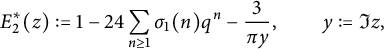 $$\begin{align*}E_{2}^{*}(z):=1-24\sum_{n\geq1}\sigma_{1}(n)q^{n}-\frac{3}{\pi y},\qquad y:=\Im z, \end{align*}$$
offers an elegant example. For a fixed fundamental discriminant $\Delta <0$
, let
$\Delta <0$
, let $\chi _{\Delta }$
be the genus character from, e.g., Section 1.2 of [Reference Gross, Kohnen and ZagierGKZ] (with
$\chi _{\Delta }$
be the genus character from, e.g., Section 1.2 of [Reference Gross, Kohnen and ZagierGKZ] (with $N=1$
), which takes
$N=1$
), which takes $\lambda \in \mathbb {Z}^{3}$
to
$\lambda \in \mathbb {Z}^{3}$
to
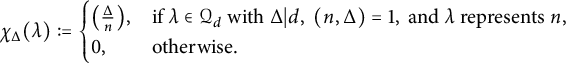 $$ \begin{align} \chi_{\Delta}(\lambda):= \begin{cases} \big(\frac{\Delta}{n}\big), & \text{if }\lambda\in\mathcal{Q}_{d}\text{ with }\Delta|d,\ (n,\Delta)=1,\text{ and }\lambda\text{ represents }n, \\ 0, & \text{otherwise}. \end{cases} \end{align} $$
Then, for any fundamental discriminant $D<0$
co-prime to
$D<0$
co-prime to $\Delta $
, we have the formula
$\Delta $
, we have the formula
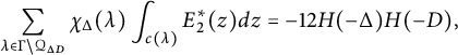 $$ \begin{align} \sum_{\lambda\in\Gamma\backslash\mathcal{Q}_{\Delta D}}\chi_{\Delta}(\lambda)\int_{c(\lambda)}E^{*}_{2}(z)dz=-12H(-\Delta)H(-D), \end{align} $$
where $H(n)$
is the Hurwitz class number considered in [Reference Hirzebruch and ZagierHZ]. This twisted cycle integral (generalizing the classical integral, in which the character is trivial) is also the
$H(n)$
is the Hurwitz class number considered in [Reference Hirzebruch and ZagierHZ]. This twisted cycle integral (generalizing the classical integral, in which the character is trivial) is also the $|D|$
th Fourier coefficient of
$|D|$
th Fourier coefficient of $12H(-\Delta )$
times the weight
$12H(-\Delta )$
times the weight $\frac {3}{2}$
mock modular form studied in loc. cit. In fact, this equality holds for any discriminant
$\frac {3}{2}$
mock modular form studied in loc. cit. In fact, this equality holds for any discriminant $D<0$
after suitably regularizing the left-hand side (see Corollary 1.12 of [Reference Alfes and EhlenANS]Footnote
1
). The modular completion of this mock modular form is a harmonic Maass form in the sense of [Reference Bruinier and FunkeBF1], whose image under the differential operator
$D<0$
after suitably regularizing the left-hand side (see Corollary 1.12 of [Reference Alfes and EhlenANS]Footnote
1
). The modular completion of this mock modular form is a harmonic Maass form in the sense of [Reference Bruinier and FunkeBF1], whose image under the differential operator $\xi _{3/2}$
(see (2.1)), also known as the shadow of the mock modular form, is a multiple of the Jacobi theta series of weight
$\xi _{3/2}$
(see (2.1)), also known as the shadow of the mock modular form, is a multiple of the Jacobi theta series of weight $\frac {1}{2}$
.
$\frac {1}{2}$
.
Note that for a fundamental discriminant $D>0$
, the twisted trace of singular moduli
$D>0$
, the twisted trace of singular moduli
 $$ \begin{align} A(D,-\Delta):=\frac{1}{\sqrt{D}}\sum_{\lambda\in\Gamma\backslash\mathcal{Q}_{\Delta D},\ \lambda\gg0}\frac{\chi_{\Delta}(\lambda)}{|\Gamma_{\lambda}|}J(z_{\lambda}) \end{align} $$
(again generalizing the usual trace, with no character) is the Dth Fourier coefficient of the weakly holomorphic modular form $f_{-\Delta }=q^{\Delta }+O(q)$
of weight
$f_{-\Delta }=q^{\Delta }+O(q)$
of weight $\frac {1}{2}$
from [Reference ZagierZa]. This coefficient is the same with
$\frac {1}{2}$
from [Reference ZagierZa]. This coefficient is the same with $J=j-744$
replaced by j when
$J=j-744$
replaced by j when $D\Delta $
is not a square.
$D\Delta $
is not a square.
While searching for analogues of the result from [Reference ZagierZa] mentioned above, Duke, Imamoğlu, and Tóth studied the generating series of cycle integrals of the j-function in [Reference Duke, Imamoğlu and TóthDIT], and showed that it is a mock modular form of weight $\frac {1}{2}$
whose shadow is the weight
$\frac {1}{2}$
whose shadow is the weight $\frac {3}{2}$
form g from [Reference ZagierZa]. Furthermore, it is the first member of a family of mock modular forms with weakly holomorphic shadows of weight
$\frac {3}{2}$
form g from [Reference ZagierZa]. Furthermore, it is the first member of a family of mock modular forms with weakly holomorphic shadows of weight $\frac {3}{2}$
.
$\frac {3}{2}$
.
Using Serre duality, it is easy to see that there is a unique mock modular form $\tilde {f}_{-\Delta }$
of weight
$\tilde {f}_{-\Delta }$
of weight $\frac {3}{2}$
and level 4 in Kohnen’s plus space with shadow
$\frac {3}{2}$
and level 4 in Kohnen’s plus space with shadow $\frac {3}{2\pi }f_{-\Delta }$
and Fourier expansion
$\frac {3}{2\pi }f_{-\Delta }$
and Fourier expansion
 $$\begin{align*}\tilde{f}_{-\Delta}(z)=48|\Delta|H(-\Delta)+O(q^{3}).\end{align*}$$
From the result in [Reference Duke, Imamoğlu and TóthDIT], it is natural to ask about ways to construction $\tilde {f}_{-\Delta }$
. This was first done by Jeon, Kang, and Kim in [Reference Jeon, Kang and KimJKK1] using Maass–Poincaré series. The sequel [Reference Jeon, Kang and KimJKK2] expressed its Fourier coefficients, using the same approach as in [Reference Duke, Imamoğlu and TóthDIT], as cycle integrals of sesqui-harmonic modular forms of weight zero.
$\tilde {f}_{-\Delta }$
. This was first done by Jeon, Kang, and Kim in [Reference Jeon, Kang and KimJKK1] using Maass–Poincaré series. The sequel [Reference Jeon, Kang and KimJKK2] expressed its Fourier coefficients, using the same approach as in [Reference Duke, Imamoğlu and TóthDIT], as cycle integrals of sesqui-harmonic modular forms of weight zero.
In [Reference Bruinier, Funke and ImamoğluBFI], Bruinier, Funke, and Imamoğlu obtained another proof of the main result of [Reference Duke, Imamoğlu and TóthDIT] by applying a theta lift, which also gave a geometric interpretation of the Fourier coefficients with square indices. This idea was used by Alfes-Neumann and Schwagenscheidt in [Reference Alfes and EhlenANS] to construct $\tilde {f}_{-\Delta }$
as the holomorphic part of the Shintani theta lift of a harmonic Maass form
$\tilde {f}_{-\Delta }$
as the holomorphic part of the Shintani theta lift of a harmonic Maass form $\tilde {J}$
of weight 2, which expresses the Fourier coefficients of
$\tilde {J}$
of weight 2, which expresses the Fourier coefficients of $\tilde {f}_{-\Delta }$
as the twisted cycle integrals of
$\tilde {f}_{-\Delta }$
as the twisted cycle integrals of $\tilde {J}$
. Our first result is another expression of the Fourier coefficients of
$\tilde {J}$
. Our first result is another expression of the Fourier coefficients of $\tilde {f}_{-\Delta }$
in terms of cycle integrals of nearly holomorphic modular forms.
$\tilde {f}_{-\Delta }$
in terms of cycle integrals of nearly holomorphic modular forms.
Theorem 1.1 Let $\Delta <0$
be a fixed fundamental discriminant. For any discriminant
$\Delta <0$
be a fixed fundamental discriminant. For any discriminant $D<0$
, the twisted regularized cycle integral
$D<0$
, the twisted regularized cycle integral
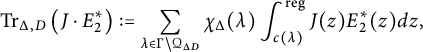 $$\begin{align*}\operatorname{Tr}_{\Delta,D}\big(J \cdot E_{2}^{*}\big):=\sum_{\lambda\in\Gamma\backslash\mathcal{Q}_{\Delta D}}\chi_{\Delta}(\lambda)\int_{c(\lambda)}^{\mathrm{reg}}J(z)E^{*}_{2}(z)dz, \end{align*}$$
with the regularization defined as in equation (4.6), is the $|D|$
th Fourier coefficient of
$|D|$
th Fourier coefficient of $\tilde {f}_{-\Delta }$
.
$\tilde {f}_{-\Delta }$
.
To prove Theorem 1.1, we will follow the theta lift approach as in [Reference Alfes and EhlenANS, Reference Bruinier and FunkeBF1, Reference Bruinier, Funke and ImamoğluBFI], and use the theta kernel with the same archimedean Schwartz function as in [Reference ShimuraSh]. (this is also the case $n = 1$
of the theta function from [Reference ZemelZe2]). We shall apply it to nearly holomorphic modular forms, and compute the resulting Fourier expansions. Recall that a real-analytic modular form f on
$n = 1$
of the theta function from [Reference ZemelZe2]). We shall apply it to nearly holomorphic modular forms, and compute the resulting Fourier expansions. Recall that a real-analytic modular form f on $\mathcal {H}$
with at most linear exponential growth near the cusps is called nearly holomorphic if it can be presented as
$\mathcal {H}$
with at most linear exponential growth near the cusps is called nearly holomorphic if it can be presented as
 $$ \begin{align} \kern1pc f(z)=\sum_{l=0}^{p}\frac{f_{l}(z)}{y^{l}}\qquad\text{with}\qquad f_{l}:\mathcal{H}\to\mathbb{C}\text{ holomorphic for }0 \leq l \leq p \end{align} $$
for some $p\in \mathbb {N}$
, which is called the depth of f if
$p\in \mathbb {N}$
, which is called the depth of f if $f_{p}$
is not identically zero. In other words, it is annihilated by the operator
$f_{p}$
is not identically zero. In other words, it is annihilated by the operator $L_{z}^{p+1}$
, where
$L_{z}^{p+1}$
, where $L_{z}$
is the lowering operator defined in (2.1). We denote the space of such modular forms of weight
$L_{z}$
is the lowering operator defined in (2.1). We denote the space of such modular forms of weight $\kappa $
with respect to
$\kappa $
with respect to $\Gamma $
by
$\Gamma $
by $\widetilde {M}_{\kappa }^{!}$
, and use the superscript
$\widetilde {M}_{\kappa }^{!}$
, and use the superscript $\leq p$
to mean the subspace of forms with depth at most p. Since these differential operators commute with the slash operators, the condition of being nearly holomorphic is purely archimedean, and can be defined for any weight, Fuchsian group, character, representation, or multiplier system.
$\leq p$
to mean the subspace of forms with depth at most p. Since these differential operators commute with the slash operators, the condition of being nearly holomorphic is purely archimedean, and can be defined for any weight, Fuchsian group, character, representation, or multiplier system.
Nearly holomorphic modular forms of depth 0 are just weakly holomorphic, and the Fourier expansions of their Shintani lifts have been computed in [Reference Alfes and EhlenANS, Reference Bruinier, Funke and ImamoğluBFI, Reference Bringmann, Guerzhoy and KaneBGK, Reference ShimuraSh]. In particular, Shintani lifts of weakly holomorphic forms are holomorphic. Moreover, the main result of [Reference Alfes and EhlenANS] shows that the Shintani lift of harmonic weak Maass forms without a special constant term is harmonic, and with this constant term, the Laplacian operator takes the lift to a unary theta function. This “sesqui-harmonicity” is also visible in the zeroth member $Z_{+}$
of the family of modular forms from [Reference Duke, Imamoğlu and TóthDIT]. We will show in Corollary 4.4 that when
$Z_{+}$
of the family of modular forms from [Reference Duke, Imamoğlu and TóthDIT]. We will show in Corollary 4.4 that when $0 \leq p<k$
, the Shintani lift of a nearly holomorphic modular form is also nearly holomorphic, and establish results analogous to the harmonic case (with or without constant terms) (see Theorem 1.2 in the Introduction, as well as Theorem 4.3, Proposition 4.5, and Remark 4.6 for the general statement). One could perhaps try to give another proof of the nearly holomorphic lift result by using the isomorphism
$0 \leq p<k$
, the Shintani lift of a nearly holomorphic modular form is also nearly holomorphic, and establish results analogous to the harmonic case (with or without constant terms) (see Theorem 1.2 in the Introduction, as well as Theorem 4.3, Proposition 4.5, and Remark 4.6 for the general statement). One could perhaps try to give another proof of the nearly holomorphic lift result by using the isomorphism
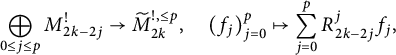 $$ \begin{align} \bigoplus_{0 \leq j \leq p}M_{2k-2j}^{!}\to\widetilde{M}_{2k}^{!,\leq p},\quad(f_{j})_{j=0}^{p}\mapsto\sum_{j=0}^{p}R_{2k-2j}^{j}f_{j}, \end{align} $$
described in, e.g., [Reference Martin and RoyerMR, Reference ZemelZe3, Reference ZemelZe7], and analyzing the effects of raising operators on theta kernels. Here, $R_{2k-2j}^{j}$
is the iterated raising operator defined in (2.2).
$R_{2k-2j}^{j}$
is the iterated raising operator defined in (2.2).
When $p \geq k$
, the map from equation (1.5) is not surjective, and misses some nearly holomorphic modular forms from the right-hand side. A particular example is the form
$p \geq k$
, the map from equation (1.5) is not surjective, and misses some nearly holomorphic modular forms from the right-hand side. A particular example is the form $J \cdot E_{2}^{*}$
in Theorem 1.1, or just
$J \cdot E_{2}^{*}$
in Theorem 1.1, or just $E_{2}^{*}$
itself. The Fourier expansions of their Shintani lifts do not follow from applying differential operators to known results, and are the main concern of this paper. In Theorem 4.3, we give the complete Fourier expansion of their Shintani lift. For the rest of the introduction, though, we will consider a special case of this result in level 1, which we now present.
$E_{2}^{*}$
itself. The Fourier expansions of their Shintani lifts do not follow from applying differential operators to known results, and are the main concern of this paper. In Theorem 4.3, we give the complete Fourier expansion of their Shintani lift. For the rest of the introduction, though, we will consider a special case of this result in level 1, which we now present.
Given $\lambda =[A,B,C]\in \mathcal {Q}_{d}$
, denote
$\lambda =[A,B,C]\in \mathcal {Q}_{d}$
, denote $\lambda (z):=Az^{2}+Bz+C$
. Suppose that
$\lambda (z):=Az^{2}+Bz+C$
. Suppose that $f\in \widetilde {M}_{2k}^{!,\leq p}$
expands as
$f\in \widetilde {M}_{2k}^{!,\leq p}$
expands as
 $$ \begin{align} f(z)=\sum_{l=0}^{p}\sum_{n\in\mathbb{Z}}c(n,l)q^{n}y^{-l}. \end{align} $$
Given $d\in \mathbb {Z}$
that is not a square, we define, for k even, the trace
$d\in \mathbb {Z}$
that is not a square, we define, for k even, the trace
 $$ \begin{align} \operatorname{Tr}_{d}(f):=\sum_{\lambda\in\Gamma\backslash\mathcal{Q}_{d}}\begin{cases} \frac{2}{|\Gamma_{\lambda}|}f(z_{\lambda}),& k=0,\ d<0, \\ \int_{c(\lambda)}f(z)\lambda(z)^{k-1} dz, & d>0,\ \sqrt{d}\not\in\mathbb{Z} \end{cases} \end{align} $$
(we shall not use the negative d case when $k>0$
). If
$k>0$
). If $d=r^{2}>0$
with
$d=r^{2}>0$
with $r\in \mathbb {N}$
, then we have
$r\in \mathbb {N}$
, then we have $\Gamma \backslash \mathcal {Q}_{d}=\{\pm [0,r,j]|0 \leq j<r-1\}$
and we define the trace as
$\Gamma \backslash \mathcal {Q}_{d}=\{\pm [0,r,j]|0 \leq j<r-1\}$
and we define the trace as
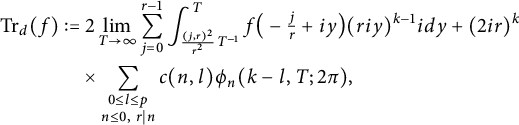 $$\begin{align*}\operatorname{Tr}_{d}(f)&:=2\lim_{T\to\infty}\sum_{j=0}^{r-1}\int_{\frac{(j,r)^{2}}{r^{2}}T^{-1}}^{T}f\big(-\tfrac{j}{r}+iy\big)(riy)^{k-1}idy+(2ir)^{k}\\& \quad \times \sum_{\substack{0 \leq l \leq p \\ n\leq0,\ r|n}}c(n,l)\phi_{n}(k-l,T;2\pi),\end{align*}$$
where the function $\phi _{n}$
is defined in equation (4.4). Finally, for
$\phi _{n}$
is defined in equation (4.4). Finally, for $d=0$
and even
$d=0$
and even $k>0$
, we set
$k>0$
, we set
 $$ \begin{align} \operatorname{Tr}_{0}(f):=c(0,0)\zeta(1-k)=-c(0,0)\frac{B_{k}}{k}, \end{align} $$
where $\zeta (s)$
is the Riemann zeta function and
$\zeta (s)$
is the Riemann zeta function and $B_{k}$
is the kth Bernoulli number.
$B_{k}$
is the kth Bernoulli number.
We can now state the Fourier expansion of the Shintani lift of $f\in \widetilde {M}_{2k}^{!,\leq p}$
for even
$f\in \widetilde {M}_{2k}^{!,\leq p}$
for even $k>0$
. For odd
$k>0$
. For odd $k\in \mathbb {N}$
, one can obtain a similar result with twisted cycle integrals as in equation (1.2).
$k\in \mathbb {N}$
, one can obtain a similar result with twisted cycle integrals as in equation (1.2).
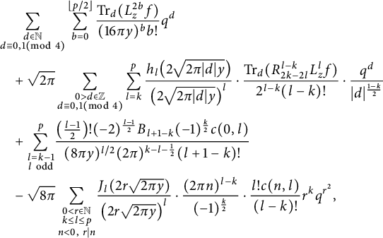
Theorem 1.2 Let $f\in \widetilde {M}_{2k}^{!,\leq p}$
have the expansion from equation (1.6), and suppose that
$f\in \widetilde {M}_{2k}^{!,\leq p}$
have the expansion from equation (1.6), and suppose that $0<k\in \mathbb {N}$
is even and
$0<k\in \mathbb {N}$
is even and $c(0,k)=0$
. The following expansion defines a real-analytic modular form of weight
$c(0,k)=0$
. The following expansion defines a real-analytic modular form of weight $k+\frac {1}{2}$
and level 4 in Kohnen’s plus space:
$k+\frac {1}{2}$
and level 4 in Kohnen’s plus space:
 $$ \begin{align*} & \sum_{\substack{d\in\mathbb{N} \\ d\equiv0,1(\mathrm{mod\ }4)}}\sum_{b=0}^{\lfloor p/2 \rfloor}\frac{\operatorname{Tr}_{d}(L_{z}^{2b}f)}{(16\pi y)^{b}b!}q^{d}\\& \quad +\sqrt{2\pi}\sum_{\substack{0>d\in\mathbb{Z} \\ d\equiv0,1(\mathrm{mod\ }4)}}\sum_{l=k}^{p}\frac{h_{l}\big(2\sqrt{2\pi|d|y}\big)}{\big(2\sqrt{2\pi|d|y}\big)^{l}}\cdot\frac{\operatorname{Tr}_{d}(R_{2k-2l}^{l-k}L_{z}^{l}f)}{2^{l-k}(l-k)!}\cdot\frac{q^{d}}{|d|^{\frac{1-k}{2}}} \\& \quad + \sum_{\substack{l=k-1 \\ l\mathrm{\ odd}}}^{p}\!\frac{\big(\frac{l-1}{2}\big)!(-2)^{\frac{l-1}{2}}B_{l+1-k}(-1)^{\frac{k}{2}}c(0,l)}{(8\pi y)^{l/2}(2\pi)^{k-l-\frac{1}{2}}(l+1-k)!} \\& \quad -\sqrt{8\pi}\sum_{\substack{0<r\in\mathbb{N} \\ k \leq l \leq p \\ n<0,\ r|n}}\!\frac{J_{l}(2r\sqrt{2\pi y})}{\big(2r\sqrt{2\pi y}\big)^{l}}\cdot\frac{(2\pi n)^{l-k}}{(-1)^{\frac{k}{2}}}\cdot\frac{l!c(n,l)}{(l-k)!}r^{k}q^{r^{2}}, \end{align*} $$
where the special functions $h_{l}$
and
$h_{l}$
and $J_{l}$
are defined in equations (3.17) and (3.31), respectively. When
$J_{l}$
are defined in equations (3.17) and (3.31), respectively. When $p<k$
, it is nearly holomorphic, of depth
$p<k$
, it is nearly holomorphic, of depth $\lfloor \frac {p}{2} \rfloor $
. Otherwise, its image under the differential operator
$\lfloor \frac {p}{2} \rfloor $
. Otherwise, its image under the differential operator $\xi _{k+1/2-2\lfloor p/2 \rfloor }L^{\lfloor p/2 \rfloor }$
is nearly holomorphic of weight
$\xi _{k+1/2-2\lfloor p/2 \rfloor }L^{\lfloor p/2 \rfloor }$
is nearly holomorphic of weight $2\lfloor \frac {p}{2} \rfloor -k+\frac {3}{2}$
and depth
$2\lfloor \frac {p}{2} \rfloor -k+\frac {3}{2}$
and depth $2\lfloor \frac {p}{2} \rfloor -k+1$
.
$2\lfloor \frac {p}{2} \rfloor -k+1$
.
Remark 1.3 Theorem 1.2 holds also for $k=0$
, once one adds to the expansion
$k=0$
, once one adds to the expansion $2\sqrt {y}$
times the constant
$2\sqrt {y}$
times the constant
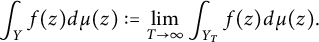 $$\begin{align*}\int_{Y}f(z)d\mu(z):=\lim_{T\to\infty}\int_{Y_{T}}f(z)d\mu(z).\end{align*}$$
Remark 1.4 In the setting of Theorem 1.2, the generating series $\sum _{d}\operatorname {Tr}_{d}(f)q^{d}$
defines, when
$\sum _{d}\operatorname {Tr}_{d}(f)q^{d}$
defines, when $p<k$
, a quasi-modular form of weight
$p<k$
, a quasi-modular form of weight $k+\frac {1}{2}$
and depth
$k+\frac {1}{2}$
and depth $\big \lfloor \frac {p}{2}\big \rfloor $
. Note that the constant term
$\big \lfloor \frac {p}{2}\big \rfloor $
. Note that the constant term $c(0,k-1)$
appearing in the third sum in Theorem 1.2 vanishes when
$c(0,k-1)$
appearing in the third sum in Theorem 1.2 vanishes when $p=k-1$
, since it is a multiple of the constant term of the weight 2 weakly holomorphic form
$p=k-1$
, since it is a multiple of the constant term of the weight 2 weakly holomorphic form $L^{k-1} f$
at the unique cusp of the modular curve of level 1. For
$L^{k-1} f$
at the unique cusp of the modular curve of level 1. For $p \geq k$
, this series can be completed to a such a modular form using these special functions (see Remark 4.7).
$p \geq k$
, this series can be completed to a such a modular form using these special functions (see Remark 4.7).
The key ingredient to the calculation of the Fourier expansion in [Reference Alfes and EhlenANS, Reference Bruinier and FunkeBF2, Reference Bruinier, Funke and ImamoğluBFI, Reference Bruinier, Funke, Imamoğlu and LiBFIL] is the construction of a rapidly decaying antiderivatives of the Schwartz function used to construct the theta kernel. Such singular Schwartz functions are important also in evaluating singular theta lifts and constructing Green currents for special divisors on orthogonal and unitary Shimura varieties (see, e.g., [Reference Funke and HofmannFH]).
In our case, we need not only the first antiderivative, but also the higher-order antiderivatives. For the first antiderivative, we can build it from the error function (see equation (3.4)). Surprisingly, the higher-order derivatives $h_{\nu }$
, defined in equation (3.17), turn out to be combinations of the Gaussian and the error function with polynomial coefficients
$h_{\nu }$
, defined in equation (3.17), turn out to be combinations of the Gaussian and the error function with polynomial coefficients $P_{\nu }$
and
$P_{\nu }$
and $Q_{\nu }$
. These polynomials, which are defined in equation (3.6), are closely related to the Hermite polynomials, and are of independent interest.
$Q_{\nu }$
. These polynomials, which are defined in equation (3.6), are closely related to the Hermite polynomials, and are of independent interest.
The paper is organized as follows. After recalling some basic notions in Section 2, we devote Section 3 to study the properties of the polynomials $P_{\nu }$
and
$P_{\nu }$
and $Q_{\nu }$
and of related special functions, including their Fourier transforms, asymptotic behaviors, and certain lattice sum evaluations. Then, in Section 4, we complete the computations of the orbital integrals and the proof of the main theorem (Theorem 4.3), as well as its implications for Theorems 1.1 and 1.2.
$Q_{\nu }$
and of related special functions, including their Fourier transforms, asymptotic behaviors, and certain lattice sum evaluations. Then, in Section 4, we complete the computations of the orbital integrals and the proof of the main theorem (Theorem 4.3), as well as its implications for Theorems 1.1 and 1.2.
2 Isotropic lattices and modular forms
This section introduces the notions and notation that are required for the rest of the paper. We follow the setup of [Reference Alfes and EhlenANS, Reference Bruinier and FunkeBF1, Reference Bruinier, Funke and ImamoğluBFI, Reference Bruinier, Funke, Imamoğlu and LiBFIL] and others.
2.1 Differential operators on modular forms
For $M=\big (\begin {smallmatrix}a & b \\ c & d\end {smallmatrix}\big )\in \operatorname {SL}_{2}(\mathbb {R})$
and an element z of
$M=\big (\begin {smallmatrix}a & b \\ c & d\end {smallmatrix}\big )\in \operatorname {SL}_{2}(\mathbb {R})$
and an element z of $\mathcal {H}:=\{z=x+iy\in \mathbb {C}|y>0\}$
, denote
$\mathcal {H}:=\{z=x+iy\in \mathbb {C}|y>0\}$
, denote $j(M,z):=cz+d$
. Let
$j(M,z):=cz+d$
. Let $\operatorname {Mp}_{2}(\mathbb {R})$
denote the metaplectic double cover of
$\operatorname {Mp}_{2}(\mathbb {R})$
denote the metaplectic double cover of $\operatorname {SL}_{2}(\mathbb {R})$
, and let
$\operatorname {SL}_{2}(\mathbb {R})$
, and let $\operatorname {Mp}_{2}(\mathbb {Z})$
be the inverse image of
$\operatorname {Mp}_{2}(\mathbb {Z})$
be the inverse image of $\operatorname {SL}_{2}(\mathbb {Z})$
in
$\operatorname {SL}_{2}(\mathbb {Z})$
in $\operatorname {Mp}_{2}(\mathbb {R})$
. We write elements of
$\operatorname {Mp}_{2}(\mathbb {R})$
. We write elements of $\operatorname {Mp}_{2}(\mathbb {R})$
as pairs
$\operatorname {Mp}_{2}(\mathbb {R})$
as pairs $(M,\phi )$
, with
$(M,\phi )$
, with $M\in \operatorname {SL}_{2}(\mathbb {R})$
and
$M\in \operatorname {SL}_{2}(\mathbb {R})$
and $\phi $
a holomorphic function on
$\phi $
a holomorphic function on $\mathcal {H}$
such that
$\mathcal {H}$
such that $\phi (z)^{2}=j(M,z)$
.
$\phi (z)^{2}=j(M,z)$
.
Given a representation $\rho $
of a finite index subgroup
$\rho $
of a finite index subgroup $\Gamma \subseteq \operatorname {Mp}_{2}(\mathbb {Z})$
on a finite-dimensional complex vector space V, a function
$\Gamma \subseteq \operatorname {Mp}_{2}(\mathbb {Z})$
on a finite-dimensional complex vector space V, a function $f:\mathcal {H} \to V$
is called modular of weight
$f:\mathcal {H} \to V$
is called modular of weight $\kappa \in \frac {1}{2}\mathbb {Z}$
and representation
$\kappa \in \frac {1}{2}\mathbb {Z}$
and representation $\rho $
if the functional equation
$\rho $
if the functional equation
 $$\begin{align*}f\mid_{\kappa}(M,\phi)(z):=\phi(z)^{-2\kappa}f(Mz)=\rho(M,\phi)f(z)\end{align*}$$
holds for every element $(M,\phi )\in \Gamma $
. Let
$(M,\phi )\in \Gamma $
. Let $\mathcal {A}_{\kappa }^{!}(\Gamma ,\rho )$
(resp.
$\mathcal {A}_{\kappa }^{!}(\Gamma ,\rho )$
(resp. $\mathcal {A}_{\kappa }(\Gamma ,\rho )$
) denote the space of such functions that are real-analytic with at most exponential (resp. polynomial) growth near the cusps. It contains the subspaces
$\mathcal {A}_{\kappa }(\Gamma ,\rho )$
) denote the space of such functions that are real-analytic with at most exponential (resp. polynomial) growth near the cusps. It contains the subspaces $\widetilde {M}_{\kappa }^{!}(\Gamma ,\rho )$
,
$\widetilde {M}_{\kappa }^{!}(\Gamma ,\rho )$
, $M_{\kappa }^{!}(\Gamma ,\rho )$
,
$M_{\kappa }^{!}(\Gamma ,\rho )$
, $M_{\kappa }(\Gamma ,\rho )$
, and
$M_{\kappa }(\Gamma ,\rho )$
, and $S_{\kappa }(\Gamma ,\rho )$
of nearly holomorphic, weakly holomorphic, holomorphic, and cusp forms, respectively. We shall omit
$S_{\kappa }(\Gamma ,\rho )$
of nearly holomorphic, weakly holomorphic, holomorphic, and cusp forms, respectively. We shall omit $\rho $
from the notation when it is trivial.
$\rho $
from the notation when it is trivial.
For a half-integer $\kappa $
, we define
$\kappa $
, we define
 $$ \begin{align} \begin{aligned} R_{z, \kappa}&= R_{\kappa} := 2i\partial_{z}+\tfrac{\kappa}{y},\qquad L=L_{z}:=-2iy^{2}\partial_{\overline{z}},\qquad\xi_{\kappa}=2iy^{\kappa} \overline{\partial_{\overline{z}}}=y^{\kappa-2}\overline{L_{z}},\qquad\text{and} \\ \Delta_{\kappa}&:=-R_{\kappa-2}L_{z}=-\xi_{2-\kappa}\xi_{\kappa}=-4y^{2}\partial_{z}+\partial_{\overline{z}}+2i\kappa y\partial_{\overline{z}}=-y^{2}(\partial_{x}^{2}+\partial_{y}^{2})-\kappa y(\partial_{y}-i\partial_{x}), \end{aligned} \end{align} $$
which are the raising operator of weight $\kappa $
, the weight lowering operator, the
$\kappa $
, the weight lowering operator, the $\xi $
-operator of weight
$\xi $
-operator of weight $\kappa $
from [Reference Bruinier and FunkeBF1], and the Laplacian operator of weight
$\kappa $
from [Reference Bruinier and FunkeBF1], and the Laplacian operator of weight $\kappa $
, respectively. For
$\kappa $
, respectively. For $n\in \mathbb {N}$
, we write
$n\in \mathbb {N}$
, we write
 $$ \begin{align} R_{\kappa}^{n}:=R_{\kappa+2n-2} \circ R_{\kappa+2n-4} \circ \dots \circ R_{\kappa+2} \circ R_{\kappa} \end{align} $$
for the iterated raising operator.
These differential operators preserve modularity, in the sense that
 $$\begin{align*}R_{\kappa}\mathcal{A}_{\kappa}^{!}(\Gamma,\rho)\subseteq\mathcal{A}_{\kappa+2}^{!}(\Gamma,\rho),\ L_{z}\mathcal{A}_{\kappa}^{!}(\Gamma,\rho)\subseteq\mathcal{A}_{\kappa-2}^{!}(\Gamma,\rho),\text{ and }\Delta_{\kappa}\mathcal{A}_{\kappa}^{!}(\Gamma,\rho)\subseteq\mathcal{A}_{\kappa}^{!}(\Gamma,\rho),\end{align*}$$
whereas for $\xi _{\kappa }$
, which involves complex conjugation, we have
$\xi _{\kappa }$
, which involves complex conjugation, we have
 $$ \begin{equation} \xi_{\kappa}\mathcal{A}_{\kappa}^{!}(\Gamma,\rho)\subseteq\mathcal{A}_{2-\kappa}^{!}(\Gamma,\overline{\rho}),\mathrm{\ where\ }\overline{\rho}\mathrm{\ is\ the\ complex\ conjugate\ representation}. \end{equation} $$
It is known that $L_{z}$
,
$L_{z}$
, $R_{\kappa }$
, and
$R_{\kappa }$
, and $\Delta _{\kappa }$
preserve near holomorphicity, with
$\Delta _{\kappa }$
preserve near holomorphicity, with $L_{z}$
decreasing the depth by 1, and
$L_{z}$
decreasing the depth by 1, and $R_{\kappa }$
and
$R_{\kappa }$
and $\Delta _{\kappa }$
increasing it by at most 1. For more on these modular forms, including their relations with quasi-modular forms and Shimura’s vector-valued modular forms, see [Reference Martin and RoyerMR, Reference ZemelZe3, Reference ZemelZe7].
$\Delta _{\kappa }$
increasing it by at most 1. For more on these modular forms, including their relations with quasi-modular forms and Shimura’s vector-valued modular forms, see [Reference Martin and RoyerMR, Reference ZemelZe3, Reference ZemelZe7].
Around a given point $w=s+it\in \mathcal {H}$
, the natural local coordinate is
$w=s+it\in \mathcal {H}$
, the natural local coordinate is
 $$ \begin{align} \zeta=A_{w}(z):=\tfrac{z-w}{z-\overline{w}}\in\big\{\zeta\in\mathbb{C}\big||\zeta|<1\big\},\qquad\mathrm{with}\qquad1-A_{w}(z)=\tfrac{2it}{z-\overline{w}} \end{align} $$
for any $z\in \mathcal {H}$
, which also satisfies
$z\in \mathcal {H}$
, which also satisfies
 $$\begin{align*}|A_{\gamma w}(\gamma z)|=\Bigg|\frac{\overline{j(\gamma,w)}A_{w}(z)}{j(\gamma,w)}\Bigg|=|A_{w}(z)| \end{align*}$$
for every z and w in $\mathcal {H}$
and
$\mathcal {H}$
and $\gamma \in \operatorname {SL}_{2}(\mathbb {R})$
. The expansion of a holomorphic modular form f of weight
$\gamma \in \operatorname {SL}_{2}(\mathbb {R})$
. The expansion of a holomorphic modular form f of weight $\kappa \in \mathbb {Z}$
is given by Proposition 17 of [Reference Bruinier, van der Geer, Harder and ZagierBGHZ]Footnote
2
as
$\kappa \in \mathbb {Z}$
is given by Proposition 17 of [Reference Bruinier, van der Geer, Harder and ZagierBGHZ]Footnote
2
as
 $$ \begin{align} f(z)=\bigg(\frac{2it}{z-\overline{w}}\bigg)^{\kappa}\sum_{n=0}^{\infty}R_{\kappa}^{n}f(w)\frac{t^{n}A_{w}(z)^{n}}{n!}=\big(1-A_{w}(z)\big)^{\kappa}\sum_{n=0}^{\infty}R_{\kappa}^{n}f(w)\frac{t^{n}A_{w}(z)^{n}}{n!}. \end{align} $$
Note that the proof of equation (2.5) makes no use of the modularity of f, so that this expansion is valid for every holomorphic function f. We shall need a formula extending equation (2.5) to nearly holomorphic modular forms.
Lemma 2.1 For $f\in \widetilde {M}^{!}_{\kappa }(\Gamma ,\rho )$
and a point
$f\in \widetilde {M}^{!}_{\kappa }(\Gamma ,\rho )$
and a point $w=s+it\in \mathcal {H}$
, we have the expansion
$w=s+it\in \mathcal {H}$
, we have the expansion
 $$\begin{align*}f(z)=\big(1-A_{w}(z)\big)^{\kappa}\sum_{l=0}^{p}\frac{\big(1-\overline{A_{w}(z)}\big)^{l}}{t^{l} \big(1-\big|A_{w}(z)\big|^{2}\big)^{l}}\sum_{n=0}^{\infty} R_{\kappa-l}^{n}f_{l}(w)\frac{t^{n}A_{w}(z)^{n}}{n!}. \end{align*}$$
Proof We write $f(z)$
as in equation (1.4), and express each
$f(z)$
as in equation (1.4), and express each $f_{l}$
via equation (2.5), but with
$f_{l}$
via equation (2.5), but with $\kappa $
replaced by
$\kappa $
replaced by $\kappa -l$
. Recalling from Lemma 5.1 of [Reference ZemelZe4] that y equals
$\kappa -l$
. Recalling from Lemma 5.1 of [Reference ZemelZe4] that y equals $\frac {t(1-|A_{w}(z)|^{2})}{|1-A_{w}(z)|^{2}}$
, we get
$\frac {t(1-|A_{w}(z)|^{2})}{|1-A_{w}(z)|^{2}}$
, we get
 $$\begin{align*}f(z)=\sum_{l=0}^{p}\frac{\big(1-A_{w}(z)\big)^{\kappa-l}\sum_{n=0}^{\infty}R_{\kappa-l}^{n}f_{l}(w)\frac{t^{n}A_{w}(z)^{n}}{n!}}{t^{l}\big(1-\big|A_{w}(z)\big|^{2}\big)^{l}}\big|1-A_{w}(z)\big|^{2l}.\end{align*}$$
Expanding $\big |1-A_{w}(z)\big |^{2}$
yields the desired result. This proves the lemma.
$\big |1-A_{w}(z)\big |^{2}$
yields the desired result. This proves the lemma.
For any $\epsilon>0$
, we will denote the pre-image of the ball of radius
$\epsilon>0$
, we will denote the pre-image of the ball of radius $\epsilon $
in
$\epsilon $
in $\mathbb {C}$
under
$\mathbb {C}$
under $A_{w}$
by
$A_{w}$
by $B_{\epsilon }(w)$
with the natural orientation on its boundary. We shall later need the limit value of the following integral, which is determined as follows.
$B_{\epsilon }(w)$
with the natural orientation on its boundary. We shall later need the limit value of the following integral, which is determined as follows.
Corollary 2.2 Let f and w be as in Lemma 2.1, and take an integer $\mu $
. Then
$\mu $
. Then
 $$\begin{align*}\lim_{\epsilon\to0}\int_{\partial B_{\epsilon}(w)}\frac{f(z)}{(1-A_{w}(z))^{\kappa-2}}A_{w}(z)^{\mu}dz=\begin{cases} -\frac{4\pi t^{|\mu|}}{(|\mu|-1)!}R_{\kappa}^{|\mu|-1}f(w), & \mu<0, \\ 0, & \mu\geq0. \end{cases} \end{align*}$$
Proof The result follows from substituting in $\zeta =A_{w}(z)$
, and thus
$\zeta =A_{w}(z)$
, and thus $dz=\frac {2it}{(1-\zeta )^{2}}d\zeta $
, inside Lemma 2.1. This proves the corollary.
$dz=\frac {2it}{(1-\zeta )^{2}}d\zeta $
, inside Lemma 2.1. This proves the corollary.
We will carry out some integrations of modular forms on $\mathcal {H}$
, with respect to the invariant measure
$\mathcal {H}$
, with respect to the invariant measure $d\mu (z):=\frac {dz \wedge d\overline {z}}{-2iy^{2}}=\frac {dxdy}{y^{2}}$
. The following standard consequence of Stokes’ theorem will be useful for evaluating some of these integrals (see, e.g., Proposition 4.1.1 of [Reference LiL]).
$d\mu (z):=\frac {dz \wedge d\overline {z}}{-2iy^{2}}=\frac {dxdy}{y^{2}}$
. The following standard consequence of Stokes’ theorem will be useful for evaluating some of these integrals (see, e.g., Proposition 4.1.1 of [Reference LiL]).
Lemma 2.3 Let $\mathcal {R}$
be a connected domain in
$\mathcal {R}$
be a connected domain in $\mathcal {H}$
whose boundary
$\mathcal {H}$
whose boundary $\partial \mathcal {R}$
is a piecewise smooth path in
$\partial \mathcal {R}$
is a piecewise smooth path in $\mathcal {H}$
(positively oriented), and assume that f, g, and G are real-analytic functions on
$\mathcal {H}$
(positively oriented), and assume that f, g, and G are real-analytic functions on $\mathcal {R}$
such that
$\mathcal {R}$
such that $g=-L_{z}G$
. Then we have the equality
$g=-L_{z}G$
. Then we have the equality
 $$\begin{align*}\int_{\mathcal{R}}f(z)g(z)d\mu(z)=\oint_{\partial\mathcal{R}}f(z)G(z)dz+\int_{\mathcal{R}}L_{z}f(z)G(z)d\mu(z). \end{align*}$$
2.2 Lattices producing modular curves
Let $V:=M_{2}(\mathbb {Q})^{0}$
be the signature
$V:=M_{2}(\mathbb {Q})^{0}$
be the signature $(2,1)$
quadratic space of trace zero matrices over
$(2,1)$
quadratic space of trace zero matrices over $\mathbb {Q}$
with quadratic form
$\mathbb {Q}$
with quadratic form $Q(\lambda ):=-N\det \lambda $
for some
$Q(\lambda ):=-N\det \lambda $
for some $0<N\in \mathbb {Q}$
. Then
$0<N\in \mathbb {Q}$
. Then $G:=\operatorname {Spin}(V)\cong \operatorname {SL}_{2}$
, and the symmetric space of G is the space of oriented negative definite lines in
$G:=\operatorname {Spin}(V)\cong \operatorname {SL}_{2}$
, and the symmetric space of G is the space of oriented negative definite lines in $V_{\mathbb {R}}:=M_{2}(\mathbb {R})^{0}$
. We can identify
$V_{\mathbb {R}}:=M_{2}(\mathbb {R})^{0}$
. We can identify $\mathcal {H}$
with the connected component of this symmetric space that contains the line spanned by
$\mathcal {H}$
with the connected component of this symmetric space that contains the line spanned by $\big (\begin {smallmatrix}0 & -1 \\ 1 & 0\end {smallmatrix}\big )$
as a positive generator, via the map taking
$\big (\begin {smallmatrix}0 & -1 \\ 1 & 0\end {smallmatrix}\big )$
as a positive generator, via the map taking $z\in \mathcal {H}$
to
$z\in \mathcal {H}$
to $\mathbb {R}Z^{\perp }(z)$
with
$\mathbb {R}Z^{\perp }(z)$
with
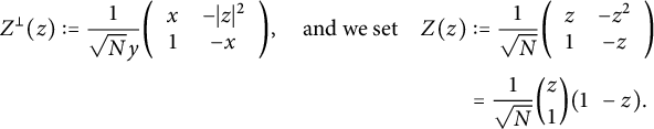 $$\begin{align*}Z^{\perp}(z):=\frac{1}{\sqrt{N}y}\bigg(\begin{array}{cc}x & -|z|^{2} \\ 1 & -x\end{array}\bigg),\quad\mathrm{and\ we\ set}\quad Z(z)&:=\frac{1}{\sqrt{N}}\bigg(\begin{array}{cc}z & -z^{2} \\ 1 & -z\end{array}\bigg)\\[3pt] & =\frac{1}{\sqrt{N}}\binom{z}{1}(1\ \ -z).\end{align*}$$
It is easy to check that $\gamma \cdot Z^{\perp }(z)=Z^{\perp }(\gamma z)$
and
$\gamma \cdot Z^{\perp }(z)=Z^{\perp }(\gamma z)$
and $\gamma \cdot Z(z)=j(\gamma ,z)^{2}Z(\gamma z)$
for every
$\gamma \cdot Z(z)=j(\gamma ,z)^{2}Z(\gamma z)$
for every $\gamma \in \operatorname {SL}_{2}(\mathbb {R})$
.
$\gamma \in \operatorname {SL}_{2}(\mathbb {R})$
.
Given $\lambda \in V_{\mathbb {R}}$
with
$\lambda \in V_{\mathbb {R}}$
with $Q(\lambda )=-\xi ^{2}<0$
, we know that
$Q(\lambda )=-\xi ^{2}<0$
, we know that $\lambda =\xi Z^{\perp }(z_{\lambda })$
for some
$\lambda =\xi Z^{\perp }(z_{\lambda })$
for some $z_{\lambda }=x_{\lambda }+iy_{\lambda }\in \mathcal {H}$
, with
$z_{\lambda }=x_{\lambda }+iy_{\lambda }\in \mathcal {H}$
, with $\operatorname {sgn}(\xi )=-\operatorname {sgn}\big (\lambda ,Z^{\perp }(z_{\lambda })\big )$
. In this case, Lemma 4.2 of [Reference ZemelZe4] proves the equalities
$\operatorname {sgn}(\xi )=-\operatorname {sgn}\big (\lambda ,Z^{\perp }(z_{\lambda })\big )$
. In this case, Lemma 4.2 of [Reference ZemelZe4] proves the equalities
 $$ \begin{align} \begin{aligned} \big(\lambda,Z^{\perp}(z)\big)&=-2\xi\cosh d(z,z_{\lambda})=-2\xi\bigg(\frac{|z-{z_{\lambda}}|^{2}}{2yy_{\lambda}}+1\bigg)=-2\xi \frac{1+|A_{{z_{\lambda}}}(z)|^{2}}{1-|A_{{z_{\lambda}}}(z)|^{2}}, \\[6pt] \big(\lambda,Z(z)\big)&=-2\xi\frac{(z-{z_{\lambda}})(z-\overline{{z_{\lambda}}})}{2y_{\lambda}}=\frac{4\xi y_{\lambda}A_{{z_{\lambda}}}(z)}{\big(1-A_{{z_{\lambda}}}(z)\big)^{2}}, \end{aligned} \end{align} $$
where $d(z,z_{\lambda })$
is the hyperbolic distance between z and
$d(z,z_{\lambda })$
is the hyperbolic distance between z and $z_{\lambda }$
.
$z_{\lambda }$
.
Fix an even, integral lattice $L \subseteq V$
, with its dual
$L \subseteq V$
, with its dual $L^{*}:=\operatorname {Hom}(L,\mathbb {Z})$
viewed as a subgroup of V containing L, and
$L^{*}:=\operatorname {Hom}(L,\mathbb {Z})$
viewed as a subgroup of V containing L, and $D_{L}:=L^{*}/L$
the associated finite quadratic module. We denote
$D_{L}:=L^{*}/L$
the associated finite quadratic module. We denote $\Gamma =\Gamma _{L} \subseteq G(\mathbb {Q})=\operatorname {SL}_{2}(\mathbb {Q})$
the inverse image of the discriminant kernelFootnote
3
of L, and set
$\Gamma =\Gamma _{L} \subseteq G(\mathbb {Q})=\operatorname {SL}_{2}(\mathbb {Q})$
the inverse image of the discriminant kernelFootnote
3
of L, and set $Y:=Y_{L}:=\Gamma \backslash \mathcal {H}$
to be the associated (open) modular curve, with the projection map
$Y:=Y_{L}:=\Gamma \backslash \mathcal {H}$
to be the associated (open) modular curve, with the projection map $\pi :\mathcal {H} \to Y$
. For every
$\pi :\mathcal {H} \to Y$
. For every $h \in D_{L}$
and
$h \in D_{L}$
and $m\in \mathbb {Z}+Q(h)$
, we denote
$m\in \mathbb {Z}+Q(h)$
, we denote
 $$ \begin{align} L_{m,h}:=\{\lambda \in L+h|Q(\lambda)=m\}. \end{align} $$
Typical examples can be found in [Reference BorcherdsBO], [Reference Alfes-Neumann and SchwagenscheidtAE], [Reference Li and ZemelLZ], or [Reference ZemelZe6]; e.g.,
 $$ \begin{align} L=\big\{\big(\begin{smallmatrix}-B & C \\ -A & B\end{smallmatrix}\big)\big|A, B, C\in\mathbb{Z}\big\}\quad\mathrm{with}\quad Q=-\det\quad\mathrm{and}\quad\Gamma=\operatorname{SL}_{2}(\mathbb{Z}). \end{align} $$
Furthermore, let $\rho _{L}$
be the Weil representation associated with L, in which
$\rho _{L}$
be the Weil representation associated with L, in which $\operatorname {Mp}_{2}(\mathbb {Z})$
operates on the vector space
$\operatorname {Mp}_{2}(\mathbb {Z})$
operates on the vector space $\mathbb {C}[D_{L}]$
, with the canonical basis
$\mathbb {C}[D_{L}]$
, with the canonical basis $\{\mathfrak {e}_{h}\}_{h \in D_{L}}$
(see [Reference BorcherdsBo, Reference ScheithauerSch, Reference StrömbergStr, Reference ZemelZe1] and others).
$\{\mathfrak {e}_{h}\}_{h \in D_{L}}$
(see [Reference BorcherdsBo, Reference ScheithauerSch, Reference StrömbergStr, Reference ZemelZe1] and others).
2.3 Cusps and geodesics
The Baily–Borel completion $\mathcal {H}^{*}$
of
$\mathcal {H}^{*}$
of $\mathcal {H}$
is obtained by adding the set
$\mathcal {H}$
is obtained by adding the set $\operatorname {Iso}(V)\cong \mathbb {P}^{1}(\mathbb {Q})$
of isotropic lines in V. Let
$\operatorname {Iso}(V)\cong \mathbb {P}^{1}(\mathbb {Q})$
of isotropic lines in V. Let $\ell _{\infty }\in \operatorname {Iso}(V)$
be the line spanned by
$\ell _{\infty }\in \operatorname {Iso}(V)$
be the line spanned by $u_{\infty }:=\big (\begin {smallmatrix} 0 & 1 \\ 0 & 0\end {smallmatrix}\big )$
, and given
$u_{\infty }:=\big (\begin {smallmatrix} 0 & 1 \\ 0 & 0\end {smallmatrix}\big )$
, and given $\ell \in \operatorname {Iso}(V)$
, we take an element
$\ell \in \operatorname {Iso}(V)$
, we take an element $\sigma _{\ell }\in \operatorname {SL}_{2}(\mathbb {Z})$
such that
$\sigma _{\ell }\in \operatorname {SL}_{2}(\mathbb {Z})$
such that $\ell =\sigma _{\ell }\ell _{\infty }$
, and set
$\ell =\sigma _{\ell }\ell _{\infty }$
, and set $u_{\ell }:=\sigma _{\ell }u_{\infty }$
. If
$u_{\ell }:=\sigma _{\ell }u_{\infty }$
. If $\Gamma _{\ell }\subseteq \Gamma \subseteq \operatorname {SL}_{2}(\mathbb {Z})$
is the stabilizer of
$\Gamma _{\ell }\subseteq \Gamma \subseteq \operatorname {SL}_{2}(\mathbb {Z})$
is the stabilizer of $\ell $
, then there exists
$\ell $
, then there exists $\alpha _{\ell }\in \mathbb {N}$
, called the width of the cusp
$\alpha _{\ell }\in \mathbb {N}$
, called the width of the cusp $\ell $
, such that
$\ell $
, such that
 $$ \begin{align} \sigma_{\ell}^{-1}\Gamma_{\ell}\sigma_{\ell}=\big\{\pm\big(\begin{smallmatrix} 1 & n\alpha_{\ell} \\ 0 & 1\end{smallmatrix}\big)\big|n\in\mathbb{Z}\big\}. \end{align} $$
Let $0<\beta _{\ell }\in \mathbb {Q}$
be such that
$0<\beta _{\ell }\in \mathbb {Q}$
be such that
 $$ \begin{align} L\cap\ell=\mathbb{Z}\beta_{\ell}u_{\ell},\quad\text{and set}\quad\varepsilon_{\ell}:=\tfrac{\alpha_{\ell}}{\beta_{\ell}}. \end{align} $$
When $(L+h)\cap \ell \neq \emptyset $
, we define
$(L+h)\cap \ell \neq \emptyset $
, we define $0 \leq k_{\ell ,h}<\beta _{\ell }$
to be the unique number such that
$0 \leq k_{\ell ,h}<\beta _{\ell }$
to be the unique number such that
 $$ \begin{align} (L+h)\cap\ell=(\mathbb{Z}\beta_{\ell}+k_{\ell,h})u_{\ell},\quad\mathrm{and\ set\quad} \omega_{\ell,h}:=\tfrac{k_{\ell,h}}{\beta_{\ell}}+\mathbb{Z}\in\mathbb{R}/\mathbb{Z}. \end{align} $$
All these parameters are constant on $\Gamma $
-orbits.
$\Gamma $
-orbits.
Near the cusp associated with $\ell \in \operatorname {Iso}(V)$
, we work with the coordinates
$\ell \in \operatorname {Iso}(V)$
, we work with the coordinates
 $$ \begin{align} z_{\ell}=x_{\ell}+iy_{\ell}:=\sigma_{\ell}^{-1}z\qquad\text{and}\qquad q_{\ell}(z_{\ell}):=\mathbf{e}\big(\tfrac{z_{\ell}}{\alpha_{\ell}}\big). \end{align} $$
For $\epsilon>0$
, we define the neighborhood
$\epsilon>0$
, we define the neighborhood $B_{\epsilon }(\ell ):=\big \{z\in \mathcal {H}\big ||q_{\ell }(z_{\ell })<\epsilon \}$
of the cusp
$B_{\epsilon }(\ell ):=\big \{z\in \mathcal {H}\big ||q_{\ell }(z_{\ell })<\epsilon \}$
of the cusp $\ell $
. The set
$\ell $
. The set
 $$ \begin{align} \mathcal{H}_{T}:=\mathcal{H}\setminus\bigcup_{\ell\in\operatorname{Iso}(V)}B_{e^{-2\pi T}}(\ell),\qquad\mathrm{for}\quad T>1, \end{align} $$
is $\Gamma $
-invariant, and
$\Gamma $
-invariant, and $Y_{T}:={\Gamma }\backslash \mathcal {H}_{T}$
is a truncated modular curve, with a fundamental domainFootnote
4
$Y_{T}:={\Gamma }\backslash \mathcal {H}_{T}$
is a truncated modular curve, with a fundamental domainFootnote
4
 $$ \begin{align} \mathcal{F}_{T}(L):=\bigcup_{\ell\in\Gamma\backslash\operatorname{Iso}(V)}\sigma_{\ell}\mathcal{F}_{T}^{\alpha_{\ell}},\qquad\mathrm{where}\qquad \mathcal{F}_{T}^{\alpha}:=\bigcup_{j=0}^{\alpha-1}\big(\begin{smallmatrix} 1 & j \\ 0 & 1\end{smallmatrix}\big)\mathcal{F}_{T} \end{align} $$
is composed, for $\alpha \in \mathbb {N}$
, of
$\alpha \in \mathbb {N}$
, of $\alpha $
translations of
$\alpha $
translations of
 $$\begin{align*}\mathcal{F}_{T}:=\big\{z=x+iy\in\mathcal{H}\big||x|\leq\tfrac{1}{2},\ |z|\geq1,\ y \leq T\}. \end{align*}$$
Remark 2.4 The assumption $\Gamma =\Gamma _{L}\subseteq \operatorname {SL}_{2}(\mathbb {Z})$
is satisfied for the large family of lattices from [Reference ZemelZe6], but not for every lattice L in V. However, the only place where we use the assumption that
$\Gamma =\Gamma _{L}\subseteq \operatorname {SL}_{2}(\mathbb {Z})$
is satisfied for the large family of lattices from [Reference ZemelZe6], but not for every lattice L in V. However, the only place where we use the assumption that $\Gamma \subseteq \operatorname {SL}_{2}(\mathbb {Z})$
is in the form of the fundamental domain from equation (2.14), with
$\Gamma \subseteq \operatorname {SL}_{2}(\mathbb {Z})$
is in the form of the fundamental domain from equation (2.14), with $T>1$
being a sufficient bound, and in the integrality of the parameter
$T>1$
being a sufficient bound, and in the integrality of the parameter $\alpha _{\ell }$
from equation (2.9). Since none of these facts are used in any proof below, our results hold equally well for more general lattices.
$\alpha _{\ell }$
from equation (2.9). Since none of these facts are used in any proof below, our results hold equally well for more general lattices.
An element $\lambda \in V_{\mathbb {R}}$
with
$\lambda \in V_{\mathbb {R}}$
with $Q(\lambda )>0$
defines a geodesic
$Q(\lambda )>0$
defines a geodesic
 $$ \begin{align} c_{\lambda}:=\big\{z\in\mathcal{H}\big|\big(\lambda,Z^{\perp}(z)\big)=0\big\}\subseteq\mathcal{H},\qquad\text{as well as}\qquad c(\lambda):=\Gamma_{\lambda} \backslash c_{\lambda} \subseteq Y, \end{align} $$
where $\Gamma _{\lambda }$
is the stabilizer of
$\Gamma _{\lambda }$
is the stabilizer of $\lambda $
in
$\lambda $
in $\Gamma $
. For
$\Gamma $
. For $\lambda _{0}=\big (\begin {smallmatrix} 1 & 0 \\ 0 & -1\end {smallmatrix}\big ) \in V$
, we orient the geodesic
$\lambda _{0}=\big (\begin {smallmatrix} 1 & 0 \\ 0 & -1\end {smallmatrix}\big ) \in V$
, we orient the geodesic $c_{\lambda _{0}}=(0,i\infty )$
to go up, and transfer this to an orientation on
$c_{\lambda _{0}}=(0,i\infty )$
to go up, and transfer this to an orientation on $c_{\lambda }$
and
$c_{\lambda }$
and $c(\lambda )$
for each such
$c(\lambda )$
for each such $\lambda \in V_{\mathbb {R}}$
via the action of
$\lambda \in V_{\mathbb {R}}$
via the action of $\operatorname {SL}_{2}(\mathbb {R})$
. We have the following well-known dichotomy.
$\operatorname {SL}_{2}(\mathbb {R})$
. We have the following well-known dichotomy.
Lemma 2.5 Let $\lambda \in V$
be such that
$\lambda \in V$
be such that $m=Q(\lambda )>0$
. If
$m=Q(\lambda )>0$
. If $m \in N\cdot (\mathbb {Q}^{\times })^{2}$
, then
$m \in N\cdot (\mathbb {Q}^{\times })^{2}$
, then $\Gamma _{\lambda }$
is the trivial subgroup
$\Gamma _{\lambda }$
is the trivial subgroup $\{\pm I\}$
, and the geodesic
$\{\pm I\}$
, and the geodesic $c_{\lambda }$
connects two cusps in
$c_{\lambda }$
connects two cusps in $\mathbb {P}^{1}(\mathbb {Q})$
. Otherwise, the image of
$\mathbb {P}^{1}(\mathbb {Q})$
. Otherwise, the image of $\Gamma _{\lambda }$
in
$\Gamma _{\lambda }$
in $\operatorname {SO}^{+}(V)\cong \operatorname {PSL}_{2}(\mathbb {Q})$
is infinite cyclic.
$\operatorname {SO}^{+}(V)\cong \operatorname {PSL}_{2}(\mathbb {Q})$
is infinite cyclic.
In the first case in Lemma 2.5, we call $\lambda $
split-hyperbolic. For
$\lambda $
split-hyperbolic. For $m\in \mathbb {Q}$
and for
$m\in \mathbb {Q}$
and for $\lambda \in V$
, we then set, by a slight abuse of notation,
$\lambda \in V$
, we then set, by a slight abuse of notation,
 $$ \begin{align} \iota(m):=\begin{cases} 1, & \text{if } \sqrt{m/N}\in\mathbb{Q}^{\times}, \\ 0, & \text{otherwise},\end{cases}\qquad\text{and}\qquad \iota(\lambda):=\begin{cases} 1, & \text{if }\lambda\text{ is split-hyperbolic}, \\ 0, & \text{otherwise}. \end{cases} \end{align} $$
If $\iota (\lambda )=1$
, then
$\iota (\lambda )=1$
, then $\lambda ^{\perp }$
is spanned by
$\lambda ^{\perp }$
is spanned by $\ell _{\lambda }$
and
$\ell _{\lambda }$
and $\ell _{-\lambda }$
in
$\ell _{-\lambda }$
in ${\mathrm {Iso}}(V)$
, which correspond to where
${\mathrm {Iso}}(V)$
, which correspond to where $c_{\lambda }$
ends and begins, respectively. If
$c_{\lambda }$
ends and begins, respectively. If $Q(\lambda )=m$
, then we have
$Q(\lambda )=m$
, then we have
 $$ \begin{align} \sigma_{\ell_{\lambda}}^{-1}\lambda=\sqrt{\tfrac{m}{N}}\big(\begin{smallmatrix} 1 & -2r_{\lambda} \\ 0 & -1\end{smallmatrix}\big)\quad\mathrm{for\ some}\quad r_{\lambda}\in\mathbb{Q},\quad\mathrm{with}\quad r_{\lambda}+\alpha_{\ell_{\lambda}}\mathbb{Z}\in\mathbb{Q}/\alpha_{\ell_{\lambda}}\mathbb{Z}\quad\mathrm{canonical}. \end{align} $$
The canonical image $r_{\lambda }+\alpha _{\ell _{\lambda }}\mathbb {Z}\in \mathbb {Q}/\alpha _{\ell _{\lambda }}\mathbb {Z}$
from equation (2.17), which we shall henceforth still denote by just
$r_{\lambda }+\alpha _{\ell _{\lambda }}\mathbb {Z}\in \mathbb {Q}/\alpha _{\ell _{\lambda }}\mathbb {Z}$
from equation (2.17), which we shall henceforth still denote by just $r_{\lambda }$
, is called the real part of
$r_{\lambda }$
, is called the real part of $c_{\lambda }$
, and it is constant on
$c_{\lambda }$
, and it is constant on $\Gamma $
-orbits.
$\Gamma $
-orbits.
For $\ell \in \operatorname {Iso}(V)$
,
$\ell \in \operatorname {Iso}(V)$
, $m\geq 0$
, and
$m\geq 0$
, and $h \in D_{L}$
, we set, for later use, the symbol
$h \in D_{L}$
, we set, for later use, the symbol
 $$ \begin{align} \iota_{\ell}(m,h):=\begin{cases} 1, & \text{there exists }\lambda \in L_{m,h}\cap\ell^{\perp},\ \text{positively oriented if } m>0, \\ 0, & \text{otherwise}. \end{cases} \end{align} $$
In other words, for $m>0$
, we have
$m>0$
, we have $\iota _{\ell }(m,h)=1$
if and only if
$\iota _{\ell }(m,h)=1$
if and only if $\ell =\ell _{\lambda }$
for some
$\ell =\ell _{\lambda }$
for some $\lambda \in L_{m,h}$
. The additive subgroup
$\lambda \in L_{m,h}$
. The additive subgroup $L\cap \ell $
acts on
$L\cap \ell $
acts on $L_{m,h} \cap \ell ^{\perp }$
, and we have the following standard result.
$L_{m,h} \cap \ell ^{\perp }$
, and we have the following standard result.
Lemma 2.6 (Lemma 3.1 of [Reference Bruinier, Funke, Imamoğlu and LiBFIL])
For $\ell \in \operatorname {Iso}(V)$
,
$\ell \in \operatorname {Iso}(V)$
, $0<m\in \mathbb {Q}$
, and
$0<m\in \mathbb {Q}$
, and $h \in D_{L}$
such that
$h \in D_{L}$
such that $\iota _{\ell }(m,h)=1$
, the natural map
$\iota _{\ell }(m,h)=1$
, the natural map $L_{m,h}\cap \ell ^{\perp } \to (L_{m,h}\cap \ell ^{\perp })/(L\cap \ell )$
factors through
$L_{m,h}\cap \ell ^{\perp } \to (L_{m,h}\cap \ell ^{\perp })/(L\cap \ell )$
factors through $\Gamma _{\ell }\backslash (L_{m,h}\cap \ell ^{\perp })$
. For every
$\Gamma _{\ell }\backslash (L_{m,h}\cap \ell ^{\perp })$
. For every $\lambda \in L_{m,h}\cap \ell ^{\perp }$
, there are
$\lambda \in L_{m,h}\cap \ell ^{\perp }$
, there are $2\sqrt {\frac {m}{N}}\varepsilon _{\ell }$
pre-images of
$2\sqrt {\frac {m}{N}}\varepsilon _{\ell }$
pre-images of $\lambda +(L\cap \ell )$
in
$\lambda +(L\cap \ell )$
in $\Gamma _{\ell }\backslash (L_{m,h}\cap \ell ^{\perp })$
, namely the images of
$\Gamma _{\ell }\backslash (L_{m,h}\cap \ell ^{\perp })$
, namely the images of $\{\lambda +j\beta _{\ell }u_{\ell }|0 \leq j\leq 2\sqrt {\frac {m}{N}}\varepsilon _{\ell }-1\}$
modulo
$\{\lambda +j\beta _{\ell }u_{\ell }|0 \leq j\leq 2\sqrt {\frac {m}{N}}\varepsilon _{\ell }-1\}$
modulo $\Gamma _{\ell }$
.
$\Gamma _{\ell }$
.
Remark 2.7 The number $2\sqrt {\frac {m}{N}}\varepsilon _{\ell }$
from Lemma 2.6 is therefore integral. Moreover, for
$2\sqrt {\frac {m}{N}}\varepsilon _{\ell }$
from Lemma 2.6 is therefore integral. Moreover, for $\ell $
, m, and h as in Lemma 2.6, take some positively oriented
$\ell $
, m, and h as in Lemma 2.6, take some positively oriented $\lambda \in L_{m,h}\cap \ell ^{\perp }$
, and let
$\lambda \in L_{m,h}\cap \ell ^{\perp }$
, and let $r_{\lambda }$
be as in equation (2.17). Then we have
$r_{\lambda }$
be as in equation (2.17). Then we have
 $$\begin{align*}\big\{r_{\mu}\big|\mu \in L_{m,h}\cap\ell^{\perp}\text{ positively oriented}\big\}=r_{\lambda}+\tfrac{\beta_{\ell}}{2}\sqrt{\tfrac{N}{m}}\mathbb{Z}\Big/\alpha_{\ell_{\lambda}}\mathbb{Z}\subseteq\mathbb{Q}/\alpha_{\ell_{\lambda}}\mathbb{Z},\end{align*}$$
a set of $2\sqrt {\frac {m}{N}}\varepsilon _{\ell }$
evenly spaced elements of
$2\sqrt {\frac {m}{N}}\varepsilon _{\ell }$
evenly spaced elements of $\mathbb {Q}/\alpha _{\ell _{\lambda }}\mathbb {Z}$
.
$\mathbb {Q}/\alpha _{\ell _{\lambda }}\mathbb {Z}$
.
2.4 Schwartz forms, theta functions, and Shintani lifts
Given $k\in \mathbb {N}$
, we can define the Schwartz function
$k\in \mathbb {N}$
, we can define the Schwartz function
 $$ \begin{align} \tilde{\varphi}_{k}(\lambda;\tau,z):=\big(\lambda,Z(z)\big)^{k}\mathbf{e}\big[Q(\lambda)\tau+\big(\lambda,Z^{\perp}(z)\big)^{2}\tfrac{iv}{2}\big] \end{align} $$
for $\lambda \in V_{\mathbb {R}}$
and
$\lambda \in V_{\mathbb {R}}$
and $\tau =u+iv\in \mathcal {H}$
, and construct the vector-valued theta function
$\tau =u+iv\in \mathcal {H}$
, and construct the vector-valued theta function
 $$ \begin{align} \Theta_{k,L}(\tau,z):=\sum_{h \in D_{L}}\Theta_{k,L,h}(\tau,z)\mathfrak{e}_{h},\quad\Theta_{k,L,h}(\tau,z):=\sqrt{v}\sum_{\lambda \in L+h}\tilde{\varphi}_{k}(\lambda;\tau,z). \end{align} $$
Theorem 4.1 of [Reference BorcherdsBo] implies that for fixed $z\in \mathcal {H}$
, we have
$z\in \mathcal {H}$
, we have $\Theta _{k,L}(\tau ,z)\in \mathcal {A}_{k+\frac {1}{2}}\big (\operatorname {Mp}_{2}(\mathbb {Z}),\rho _{L}\big )$
, whereas for fixed
$\Theta _{k,L}(\tau ,z)\in \mathcal {A}_{k+\frac {1}{2}}\big (\operatorname {Mp}_{2}(\mathbb {Z}),\rho _{L}\big )$
, whereas for fixed $\tau \in \mathcal {H}$
, it is easy to verify that
$\tau \in \mathcal {H}$
, it is easy to verify that $\Theta _{k,L,h}(\tau ,z)\in \mathcal {A}_{-2k}(\Gamma )$
for every
$\Theta _{k,L,h}(\tau ,z)\in \mathcal {A}_{-2k}(\Gamma )$
for every $h \in D_{L}$
. After collecting terms, we can use equation (2.7) to rewrite
$h \in D_{L}$
. After collecting terms, we can use equation (2.7) to rewrite
 $$ \begin{align} \Theta_{k,L,h}(\tau,z)=\sqrt{v}\sum_{m\in\mathbb{Z}+Q(h)}\bigg[\sum_{\lambda \in L_{m,h}}\big(\lambda,Z(z)\big)^{k}e^{-\pi v(\lambda,Z^{\perp}(z))^{2}}\bigg]q_{\tau}^{m},\quad q_{\tau}:=\mathbf{e}(\tau). \end{align} $$
Recall that the (probabilists’) Hermite polynomials are defined as
 $$ \begin{align} \operatorname{He}_{n}(\xi):=(-1)^{n}e^{\xi^{2}/2}\big(\tfrac{d}{d\xi}\big)^{n}e^{-\xi^{2}/2}=\big(\xi-\tfrac{d}{d\xi}\big)^{n}\cdot1=\sum_{b=0}^{\lfloor n/2 \rfloor}\frac{(-1)^{b}n!}{b!(n-2b)!2^{b}}\xi^{n-2b}. \end{align} $$
Then, for $\ell \in \operatorname {Iso}(V)$
and
$\ell \in \operatorname {Iso}(V)$
and $k\in \mathbb {N}$
, one defines the unary theta function
$k\in \mathbb {N}$
, one defines the unary theta function
 $$ \begin{align} \begin{aligned} \Theta_{k,\ell}(\tau)&:=\sum_{\lambda \in (L^{*}\cap\ell^{\perp})/(L^{*}\cap\ell)}\frac{\operatorname{He}_{k}\big(\sqrt{2\pi v}(\sigma_{\ell}^{-1}\lambda,\Im(Z(i)))\big)}{(2\pi v)^{k/2}}q_{\tau}^{Q(\lambda)}\sum_{\substack{h \in D_{L}\\ h+(L^{*} \cap \ell)/(L \cap \ell)=\lambda}}\mathfrak{e}_{h} \\ &=\sum_{h \in D_{L}}\sum_{\substack{0 \leq m\in\mathbb{Z}+Q(h) \\ \iota(m)=1}}a (\Theta_{k,\ell},m,h,v)q_{\tau}^{m}\mathfrak{e}_{h}\in\mathcal{A}_{k+\frac{1}{2}} \big(\operatorname{Mp}_{2}(\mathbb{Z}),\rho_{L}\big),\qquad\text{with} \\ a &(\Theta_{k,\ell},m,h,v):=\frac{\operatorname{He}_{k}\big(2\sqrt{2\pi mv}\big)}{(2\pi v)^{k/2}}\begin{cases} \big(\iota_{\ell}(m,h)+(-1)^{k}\iota_{\ell}(m,-h)\big), & m>0, \\ \iota_{\ell}(0,h),& m=0. \end{cases} \end{aligned} \end{align} $$
Remark 2.8 The theta functions $\Theta _{Sh}(\tau ,z)$
and
$\Theta _{Sh}(\tau ,z)$
and $\Theta _{\ell ,k}(\tau )$
from equations (4.1) and (4.2) of [Reference Alfes and EhlenANS] correspond to
$\Theta _{\ell ,k}(\tau )$
from equations (4.1) and (4.2) of [Reference Alfes and EhlenANS] correspond to $(-\sqrt {N}/y^{2})^{k+1}\overline {\Theta _{k+1,L}(\tau ,z)}$
,
$(-\sqrt {N}/y^{2})^{k+1}\overline {\Theta _{k+1,L}(\tau ,z)}$
, $(-i\sqrt {N})^{k}\overline {\Theta _{k,\ell }(\tau )}$
, and equation (2.23), respectively, in our setting.
$(-i\sqrt {N})^{k}\overline {\Theta _{k,\ell }(\tau )}$
, and equation (2.23), respectively, in our setting.
The function $\Theta _{k,\ell }$
from equation (2.23) appears in the asymptotic expansion of the theta kernel
$\Theta _{k,\ell }$
from equation (2.23) appears in the asymptotic expansion of the theta kernel $\Theta _{k,L}$
from (2.20), as is given in the following result. It is essentially part (2) of Proposition 4.2 of [Reference Alfes and EhlenANS], which refers to Theorem 5.2 of [Reference BorcherdsBo] for the proof, and can also be proved using properties of appropriate variants of the lattice sums from equation (3.34) below.
$\Theta _{k,L}$
from (2.20), as is given in the following result. It is essentially part (2) of Proposition 4.2 of [Reference Alfes and EhlenANS], which refers to Theorem 5.2 of [Reference BorcherdsBo] for the proof, and can also be proved using properties of appropriate variants of the lattice sums from equation (3.34) below.
Lemma 2.9 Given $\ell \in \operatorname {Iso}(V)$
, there exists a constant
$\ell \in \operatorname {Iso}(V)$
, there exists a constant $C_{\ell }>0$
such that
$C_{\ell }>0$
such that
 $$\begin{align*}(\Theta_{k,L}\mid_{2k,z}\sigma_{\ell})(\tau,z_{\ell})= \frac{i^{k}y_{\ell}^{k+1}}{\sqrt{N}\beta_{\ell}}\Theta_{k,\ell}(\tau)+O(e^{-C_{\ell}y_{\ell}^{2}}) \quad\mathrm{as}\quad y_{\ell}\to\infty. \end{align*}$$
For $f\in \mathcal {A}_{2k}^{!}(\Gamma )$
, we follow [Reference Alfes and EhlenANS, Reference Bruinier, Funke and ImamoğluBFI] (among others) to define its regularized Shintani lift, using the fundamental domain from equation (2.14), to be the theta integral
$f\in \mathcal {A}_{2k}^{!}(\Gamma )$
, we follow [Reference Alfes and EhlenANS, Reference Bruinier, Funke and ImamoğluBFI] (among others) to define its regularized Shintani lift, using the fundamental domain from equation (2.14), to be the theta integral
 $$ \begin{align} \mathcal{I}_{k,L}(\tau,f):=\sum_{\ell\in\Gamma\backslash\operatorname{Iso}(V)}\operatorname{CT}_{s=0}\bigg[\lim_{T\to\infty}\int_{\mathcal{F}_{T}^{\alpha_{\ell}}}(f\mid_{2k}\sigma_{\ell})(z_{\ell}) (\Theta_{k,L}\mid_{-2k}\sigma_{\ell})(\tau,z_{\ell})y_{\ell}^{-s}d\mu(z_{\ell})\bigg], \end{align} $$
which is an element of $\mathcal {A}_{k+\frac {1}{2}}\big (\operatorname {Mp}_{2}(\mathbb {Z}),\rho _{L}\big )$
. When the constant term of f at every cusp is zero, the integral converges absolutely and no regularization is necessary (see Proposition 4.1 of [Reference Bruinier and FunkeBF2]).
$\mathcal {A}_{k+\frac {1}{2}}\big (\operatorname {Mp}_{2}(\mathbb {Z}),\rho _{L}\big )$
. When the constant term of f at every cusp is zero, the integral converges absolutely and no regularization is necessary (see Proposition 4.1 of [Reference Bruinier and FunkeBF2]).
3 Special functions
In this section, we construct singular Schwartz functions that serve as higher-order antiderivatives of the ones appearing in the theta kernel. This requires the study of several families of polynomials and a few types of special functions and their properties, including their Fourier transforms and lattice sums. All of these expressions show up in the evaluation of the various parts of the Shintani lift of nearly holomorphic modular forms in Section 4.
3.1 Familiar functions
Let $\mathrm {g}(\xi )$
denote the Gaussian
$\mathrm {g}(\xi )$
denote the Gaussian $e^{-\xi ^{2}/2}$
. For
$e^{-\xi ^{2}/2}$
. For $\xi>0$
, it has the antiderivative
$\xi>0$
, it has the antiderivative
 $$ \begin{align} -\frac{\sqrt{\pi}}{\sqrt{2}}\cdot\operatorname{erfc}\big(\tfrac{\xi}{\sqrt{2}}\big)=-\int_{\xi}^{\infty}e^{-w^{2}/2}dw=-\int_{\xi^{2}/2}^{\infty}e^{-s}\frac{ds}{\sqrt{2s}}= -\frac{1}{\sqrt{2}}\Gamma\big(\tfrac{1}{2},\tfrac{\xi^{2}}{2}\big), \end{align} $$
where $\operatorname {erfc}$
is the complementary error function and
$\operatorname {erfc}$
is the complementary error function and $\Gamma (\mu ,t)$
is the incomplete Gamma function defined as
$\Gamma (\mu ,t)$
is the incomplete Gamma function defined as
 $$\begin{align*}\Gamma(\mu,t):=\int_{t}^{\infty}e^{-s}s^{\mu}\frac{ds}{s}\end{align*}$$
for $t>0$
. If
$t>0$
. If $0<\mu \in \mathbb {N}$
, then this formula is well defined for every
$0<\mu \in \mathbb {N}$
, then this formula is well defined for every $t\in \mathbb {R}$
, and for
$t\in \mathbb {R}$
, and for $\mu \in \mathbb {Z}$
, it is meaningful for
$\mu \in \mathbb {Z}$
, it is meaningful for $t<0$
as follows: If
$t<0$
as follows: If $\mu =0$
, then the integral is defined using the Cauchy principal value, and for smaller
$\mu =0$
, then the integral is defined using the Cauchy principal value, and for smaller $\mu $
, we employ repeated integration by parts. The explicit formulae are given by
$\mu $
, we employ repeated integration by parts. The explicit formulae are given by
 $$ \begin{align} \Gamma(\mu,t)= \begin{cases} e^{-t}(\mu-1)!\sum_{a=0}^{\mu-1}\frac{t^{a}}{a!}=e^{-t}t^{\mu}\big(1-\tfrac{d}{dt}\big)^{\mu-1}\tfrac{1}{t}, & \text{ when }0<\mu\in\mathbb{N}\text{ and }t\in\mathbb{R}, \\ \frac{(-1)^{\mu}}{|\mu|!}\bigg(\Gamma(0,t)+e^{-t}\sum_{a=0}^{|\mu|-1}\frac{a!}{(-t)^{a+1}}\bigg), & \text{ when }-\mu\in\mathbb{N},\text{ and }t\neq0, \end{cases} \end{align} $$ $\Gamma (0,t)$
can also be written as
$\Gamma (0,t)$
can also be written as $-\operatorname {Ei}(-t)$
using the exponential integral
$-\operatorname {Ei}(-t)$
using the exponential integral $\operatorname {Ei}(t):=-\int _{-t}^{\infty }e^{-w}\frac {dw}{w}$
, and the equality
$\operatorname {Ei}(t):=-\int _{-t}^{\infty }e^{-w}\frac {dw}{w}$
, and the equality
 $$ \begin{align} \tfrac{d}{dt}\Gamma(\mu,t)=-e^{-t}t^{\mu-1} \end{align} $$
holds whenever $\Gamma (\mu ,t)$
is defined.
$\Gamma (\mu ,t)$
is defined.
Modifying the antiderivative from equation (3.1), we now define
 $$ \begin{align} \mathrm{e}(\xi):=-\tfrac{\operatorname{sgn}(\xi)}{\sqrt{2}}\Gamma\big(\tfrac{1}{2},\tfrac{\xi^{2}}{2}\big)=-\operatorname{sgn}(\xi)\int_{|\xi|}^{\infty}e^{-w^{2}/2}dw\quad\mathrm{for}\quad\xi\neq0. \end{align} $$
It decays rapidly as $|\xi |\to \infty $
, but it is discontinuous at
$|\xi |\to \infty $
, but it is discontinuous at $\xi =0$
with the jump
$\xi =0$
with the jump
 $$\begin{align*}\lim_{\xi\to0^{+}}\mathrm{e}(\xi)-\lim_{\xi\to0^{-}}\mathrm{e}(\xi)=-\sqrt{2}\Gamma\big(\tfrac{1}{2},0\big)=-\sqrt{2\pi}.\end{align*}$$
We therefore have, as distributions on $\mathbb {R}$
, the equality
$\mathbb {R}$
, the equality
 $$ \begin{align} \tfrac{d}{d\xi}\mathrm{e}(\xi)=\mathrm{g}(\xi)-\sqrt{2\pi}\cdot\delta(\xi), \end{align} $$
where $\delta (\xi )$
is the Dirac delta distribution. Our next goal is to find higher-order antiderivatives of
$\delta (\xi )$
is the Dirac delta distribution. Our next goal is to find higher-order antiderivatives of $\mathrm {g}(\xi )$
.
$\mathrm {g}(\xi )$
.
3.2 Two families of polynomials
First, we will consider two sequences of polynomials in $\mathbb {Q}[\xi ]$
, which we denote by
$\mathbb {Q}[\xi ]$
, which we denote by $P_{\nu }$
and
$P_{\nu }$
and $Q_{\nu }$
with
$Q_{\nu }$
with $\nu \in \mathbb {N}$
and defined recursively as follows. They will show up in equation (3.17) and Proposition 3.14, whence their importance. Set
$\nu \in \mathbb {N}$
and defined recursively as follows. They will show up in equation (3.17) and Proposition 3.14, whence their importance. Set
 $$ \begin{align} \begin{aligned} P_{0}(\xi) &=1\quad\text{and}\quad Q_{0}(\xi)=0, \qquad\text{as well as} \\ P_{\nu}'(\xi) &=P_{\nu-1}(\xi)\quad\text{and}\quad P_{\nu}(\xi)+Q_{\nu}'(\xi)-\xi Q_{\nu}(\xi)=Q_{\nu-1}(\xi)\text{ for }\nu\geq1. \end{aligned} \end{align} $$
The fact that equation (3.6) defines unique sequences of polynomials, and their parity properties, are established via the following lemma.
Lemma 3.1 Let p and q be two polynomials in $\mathbb {Q}[\xi ]$
. Then there is a unique pair
$\mathbb {Q}[\xi ]$
. Then there is a unique pair $(P,Q)$
of polynomials P and Q such that
$(P,Q)$
of polynomials P and Q such that $P'=p$
and
$P'=p$
and $P+Q'-\xi Q=q$
. Moreover, if p and q have opposite parities, then so do P and Q, with that of P (resp. Q) coinciding with that of q (resp. p). In addition, if
$P+Q'-\xi Q=q$
. Moreover, if p and q have opposite parities, then so do P and Q, with that of P (resp. Q) coinciding with that of q (resp. p). In addition, if $p\neq 0$
has leading coefficient r and
$p\neq 0$
has leading coefficient r and $\deg q\leq \deg p$
, then
$\deg q\leq \deg p$
, then $\deg P=\deg Q+1=\deg p+1$
and the leading coefficients of both P and Q are
$\deg P=\deg Q+1=\deg p+1$
and the leading coefficients of both P and Q are $\frac {r}{\deg P}$
.
$\frac {r}{\deg P}$
.
Proof Let $\mathrm {g}(\xi ):=e^{-\xi ^{2}/2}$
denote the usual Gaussian. Then, for each
$\mathrm {g}(\xi ):=e^{-\xi ^{2}/2}$
denote the usual Gaussian. Then, for each $k\geq 1$
, the polynomial
$k\geq 1$
, the polynomial
 $$\begin{align*}p_{k}(\xi):=\mathrm{g}(\xi)^{-1}\frac{d}{d\xi}\big(\mathrm{g}(\xi)\xi^{k-1}\big)=(k-1)\xi^{k-2}-\xi^{k}\in\mathbb{Q}[\xi]\end{align*}$$
has degree k, parity $(-1)^{k}$
, and leading coefficient
$(-1)^{k}$
, and leading coefficient $-1$
. It is thus clear that
$-1$
. It is thus clear that $\{1\}\cup \{p_{k}\}_{k\geq 1}$
is a basis of
$\{1\}\cup \{p_{k}\}_{k\geq 1}$
is a basis of $\mathbb {Q}[\xi ]$
over
$\mathbb {Q}[\xi ]$
over $\mathbb {Q}$
, that respects the parity decomposition. Therefore, there exist unique
$\mathbb {Q}$
, that respects the parity decomposition. Therefore, there exist unique $\tilde {P}\in \mathbb {Q}[\xi ]$
,
$\tilde {P}\in \mathbb {Q}[\xi ]$
, $c\in \mathbb {Q}$
, and
$c\in \mathbb {Q}$
, and $Q\in \mathbb {Q}[\xi ]$
such that
$Q\in \mathbb {Q}[\xi ]$
such that
 $$\begin{align*}\tilde{P}'=p,\quad\tilde{P}(0)=0,\quad\mathrm{and}\quad\mathrm{g}(\xi)\big(q(\xi)-\tilde{P}(\xi)+c)&=\frac{d}{d\xi}\big(\mathrm{g}(\xi)Q(\xi)\big)\\ & =\mathrm{g}(\xi)\big(Q'(\xi)-\xi Q(\xi)\big).\end{align*}$$
Setting $P:=\tilde {P}-c$
proves the first assertion. For even q and odd p,
$P:=\tilde {P}-c$
proves the first assertion. For even q and odd p, $\tilde {P}$
and P are also even, and Q is thus odd. If q is odd and p is even, then
$\tilde {P}$
and P are also even, and Q is thus odd. If q is odd and p is even, then $\tilde {P}$
is also odd, and then integrating from
$\tilde {P}$
is also odd, and then integrating from $-\infty $
to
$-\infty $
to $\infty $
shows that
$\infty $
shows that $c=0$
in this case, completing the proof of the parity assertion. The assertion about the degrees and the leading coefficients when
$c=0$
in this case, completing the proof of the parity assertion. The assertion about the degrees and the leading coefficients when $\deg q\leq \deg p$
are now easily checked from this construction. This proves the lemma.
$\deg q\leq \deg p$
are now easily checked from this construction. This proves the lemma.
Corollary 3.2 Equation (3.6) defines unique sequences $\{P_{\nu }\}_{\nu =0}^{\infty }$
and
$\{P_{\nu }\}_{\nu =0}^{\infty }$
and $\{Q_{\nu }\}_{\nu =0}^{\infty }$
of polynomials in
$\{Q_{\nu }\}_{\nu =0}^{\infty }$
of polynomials in $\xi $
. Moreover,
$\xi $
. Moreover, $P_{\nu }$
is a polynomial of degree
$P_{\nu }$
is a polynomial of degree $\nu $
with leading coefficient
$\nu $
with leading coefficient $\frac {1}{\nu !}$
and parity
$\frac {1}{\nu !}$
and parity $(-1)^{\nu }$
for any
$(-1)^{\nu }$
for any $\nu \geq 0$
, and
$\nu \geq 0$
, and $Q_{\nu }$
is a polynomial of degree
$Q_{\nu }$
is a polynomial of degree $\nu -1$
with leading coefficient
$\nu -1$
with leading coefficient $\frac {1}{\nu !}$
and parity
$\frac {1}{\nu !}$
and parity $(-1)^{\nu -1}$
for any
$(-1)^{\nu -1}$
for any $\nu \geq 1$
.
$\nu \geq 1$
.
Proof All the statements hold for $\nu =0$
by equation (3.6), and once they hold for
$\nu =0$
by equation (3.6), and once they hold for $\nu -1$
, taking
$\nu -1$
, taking $p=P_{\nu -1}$
and
$p=P_{\nu -1}$
and $q=Q_{\nu -1}$
in Lemma 3.1 determines
$q=Q_{\nu -1}$
in Lemma 3.1 determines $P_{\nu }$
and
$P_{\nu }$
and $Q_{\nu }$
as P and Q, respectively, with the required properties. This proves the corollary.
$Q_{\nu }$
as P and Q, respectively, with the required properties. This proves the corollary.
For convenience, we list the polynomials $P_{\nu }$
and
$P_{\nu }$
and $Q_{\nu }$
for
$Q_{\nu }$
for $0\leq \nu \leq 4$
:
$0\leq \nu \leq 4$
:
 $$ \begin{align*} P_{0}(\xi)&=1,~ P_{1}(\xi)=\xi,~ P_{2}(\xi)=\frac{\xi^{2}+1}{2},~ P_{3}(\xi)=\frac{\xi^{3}+3\xi}{6},~ P_{4}(\xi)=\frac{\xi^{4}+6\xi^{2}+3}{24},\\ Q_{0}(\xi)&=0,~ Q_{1}(\xi)=1,~ Q_{2}(\xi)=\frac{\xi}{2},~ Q_{3}(\xi)=\frac{\xi^{2}+2}{6},~ Q_{4}(\xi)=\frac{\xi^{3}+5\xi}{24}. \end{align*} $$
It will be useful for us to consider the (ordinary) generating series
 $$ \begin{align} \Psi(\xi,t):=\sum_{\nu=0}^{\infty}P_{\nu}(\xi)t^{\nu}\qquad\text{and}\qquad\Upsilon(\xi,t):=\sum_{\nu=0}^{\infty}Q_{\nu}(\xi)t^{\nu}, \end{align} $$
considered, at the moment, as formal power series in $\xi $
and t, on which derivatives operate in the usual, formal way. They can be characterized in the following way.
$\xi $
and t, on which derivatives operate in the usual, formal way. They can be characterized in the following way.
Proposition 3.3 The formal power series $\Psi =\Psi (\xi ,t)$
(resp.
$\Psi =\Psi (\xi ,t)$
(resp. $\Upsilon =\Upsilon (\xi ,t)$
) is characterized as the unique real-analytic function satisfying the following properties:
$\Upsilon =\Upsilon (\xi ,t)$
) is characterized as the unique real-analytic function satisfying the following properties:
-
(i) For each power $t^{\nu }$
of t, the power series in
$\xi $
that multiplies it is finite, i.e., a polynomial.
$t^{\nu }$
of t, the power series in
$\xi $
that multiplies it is finite, i.e., a polynomial. -
(ii) At
$t=0$
, we have the equality
$\Psi (\xi ,0)=1$
(resp.
$\Upsilon (\xi ,0)=0$
) as series in
$\xi $
. -
(iii) The power series satisfies the differential equation
$$\begin{align*}\kern-1pc\partial_{\xi}\Psi(\xi,t)=t\cdot\Psi(\xi,t)\quad(\mathrm{resp.}\quad \Psi(\xi,t)+\partial_{\xi}\Upsilon(\xi,t)-\xi\cdot\Upsilon(\xi,t)=1+t\cdot\Upsilon(\xi,t)). \end{align*}$$


Proof Assume that $\Psi $
and
$\Psi $
and $\Upsilon $
satisfy these properties, and write their expansion in t as in equation (3.7), with polynomial coefficients
$\Upsilon $
satisfy these properties, and write their expansion in t as in equation (3.7), with polynomial coefficients $\tilde {P}_{\nu }(\xi )$
and
$\tilde {P}_{\nu }(\xi )$
and $\tilde {Q}_{\nu }(\xi )$
, respectively, by Property
$\tilde {Q}_{\nu }(\xi )$
, respectively, by Property $(i)$
. Now, Property
$(i)$
. Now, Property $(ii)$
implies that
$(ii)$
implies that $\tilde {P}_{\nu }$
and
$\tilde {P}_{\nu }$
and $\tilde {Q}_{\nu }$
satisfy the condition for
$\tilde {Q}_{\nu }$
satisfy the condition for $\nu =0$
in equation (3.6), and also explain the existence of the term 1 in the differential equation for
$\nu =0$
in equation (3.6), and also explain the existence of the term 1 in the differential equation for $\Upsilon $
in Property
$\Upsilon $
in Property $(iii)$
(set
$(iii)$
(set $t=0$
there). Next, comparing the coefficient of
$t=0$
there). Next, comparing the coefficient of $t^{\nu }$
with
$t^{\nu }$
with $\nu \geq 1$
in the series resulting from substituting these expansions into the differential equations from Property
$\nu \geq 1$
in the series resulting from substituting these expansions into the differential equations from Property $(iii)$
yields the other part of equation (3.6). Hence,
$(iii)$
yields the other part of equation (3.6). Hence, $\{\tilde {P}_{\nu }\}_{\nu =0}^{\infty }$
and
$\{\tilde {P}_{\nu }\}_{\nu =0}^{\infty }$
and $\{\tilde {Q}_{\nu }\}_{\nu =0}^{\infty }$
are sequences satisfying that equation, so that
$\{\tilde {Q}_{\nu }\}_{\nu =0}^{\infty }$
are sequences satisfying that equation, so that $\tilde {P}_{\nu }=P_{\nu }$
and
$\tilde {P}_{\nu }=P_{\nu }$
and $\tilde {Q}_{\nu }=Q_{\nu }$
for every
$\tilde {Q}_{\nu }=Q_{\nu }$
for every $\nu \in \mathbb {N}$
by Corollary 3.2. This proves the proposition.
$\nu \in \mathbb {N}$
by Corollary 3.2. This proves the proposition.
Proposition 3.3 allows us to determine the series $\Psi $
and
$\Psi $
and $\Upsilon $
explicitly as the expansions of real-analytic functions, which also shows that their Taylor expansion in (3.7) converges absolutely for all t and
$\Upsilon $
explicitly as the expansions of real-analytic functions, which also shows that their Taylor expansion in (3.7) converges absolutely for all t and $\xi $
.
$\xi $
.
Regarding Property (i) in that proposition, see Remark 3.5.
Theorem 3.4 The power series $\Psi $
and
$\Psi $
and $\Upsilon $
from equation (3.7) describe the functions
$\Upsilon $
from equation (3.7) describe the functions
 $$\begin{align*}\Psi(\xi,t)=e^{\xi t+t^{2}/2}\qquad\mathrm{and}\qquad\Upsilon(\xi,t)&=e^{(\xi+t)^{2}/2}\int_{\xi}^{\xi+t}e^{-w^{2}/2}dw\\ & = e^{\xi t+t^{2}/2}\int_{0}^{t}e^{-\xi w-w^{2}/2}dw. \end{align*}$$
These functions also satisfy the differential equations
 $$\begin{align*}(\partial_{t}-\xi)\Psi(\xi,t)=t\Psi(\xi,t)\qquad\mathrm{and}\qquad(\partial_{t}-\xi)\Upsilon(\xi,t)=t\Upsilon(\xi,t)+1. \end{align*}$$
Proof It suffices to show that the asserted series have the properties from Proposition 3.3. Property $(ii)$
is immediate for both (by substituting
$(ii)$
is immediate for both (by substituting $t=0$
), Property
$t=0$
), Property $(i)$
for
$(i)$
for $\Psi $
is easy to check by expanding it in t, and the two differential equations (that from Property
$\Psi $
is easy to check by expanding it in t, and the two differential equations (that from Property $(iii)$
and the one asserted here) are easily established by simple differentiation. Differentiation also shows that
$(iii)$
and the one asserted here) are easily established by simple differentiation. Differentiation also shows that
 $$\begin{align*}\partial_{\xi}\Upsilon(\xi,t)=(\xi+t)\Upsilon(\xi,t)+e^{(\xi+t)^{2}/2}\big[e^{-(\xi+t)^{2}/2}-e^{-\xi^{2}/2}\big]=(\xi+t)\Upsilon(\xi,t)+1-\Psi(\xi,t),\end{align*}$$
from which Property $(iii)$
for
$(iii)$
for $\Upsilon $
quickly follows.
$\Upsilon $
quickly follows.
Next, note that Property $(i)$
for
$(i)$
for $\Upsilon $
is equivalent to
$\Upsilon $
is equivalent to $\partial _{t}^{\nu }\Upsilon (\xi ,t)\big |_{t=0}$
being a polynomial in
$\partial _{t}^{\nu }\Upsilon (\xi ,t)\big |_{t=0}$
being a polynomial in $\xi $
for every
$\xi $
for every $\nu \in \mathbb {N}$
. To see this, we first evaluate
$\nu \in \mathbb {N}$
. To see this, we first evaluate $\partial _{t}\Upsilon (\xi ,t)$
as
$\partial _{t}\Upsilon (\xi ,t)$
as $1+(\xi +t)\Upsilon (\xi ,t)$
, yielding the remaining differential equation as well. Simple induction now shows that, for every
$1+(\xi +t)\Upsilon (\xi ,t)$
, yielding the remaining differential equation as well. Simple induction now shows that, for every $\nu $
, the derivative
$\nu $
, the derivative $\partial _{t}^{\nu }\Upsilon (\xi ,t)$
is a polynomial in
$\partial _{t}^{\nu }\Upsilon (\xi ,t)$
is a polynomial in $\xi +t$
plus another polynomial in
$\xi +t$
plus another polynomial in $\xi +t$
times
$\xi +t$
times $\Upsilon (\xi ,t)$
. After substituting
$\Upsilon (\xi ,t)$
. After substituting $t=0$
, the fact that
$t=0$
, the fact that $\Upsilon (\xi ,0)=0$
yields the desired assertion. This proves the theorem.
$\Upsilon (\xi ,0)=0$
yields the desired assertion. This proves the theorem.
Remark 3.5 If one considers Property $(iii)$
from Proposition 3.3 as differential equations for functions, then solving them implies that there exist functions
$(iii)$
from Proposition 3.3 as differential equations for functions, then solving them implies that there exist functions $\psi (t)$
and
$\psi (t)$
and $\phi (t)$
such that as functions,
$\phi (t)$
such that as functions, $\Psi (\xi ,t)$
and
$\Psi (\xi ,t)$
and $\Upsilon (\xi ,t)$
are
$\Upsilon (\xi ,t)$
are
 $$\begin{align*}\psi(t)e^{\xi t+t^{2}/2}\quad\mathrm{and}\quad e^{(\xi+t)^{2}/2}\Bigg[\phi(t)+\int_{\xi}^{\xi+t}e^{-w^{2}/2}dw+\big(\psi(t)-1\big)\int_{\xi}^{\infty}e^{-w^{2}/2}dw\Bigg], \end{align*}$$
respectively. The initial conditions from Property $(ii)$
amount to the equalities
$(ii)$
amount to the equalities $\psi (0)=1$
and
$\psi (0)=1$
and $\phi (0)=0$
. Showing that the polynomial property of the Taylor expansions from Property
$\phi (0)=0$
. Showing that the polynomial property of the Taylor expansions from Property $(i)$
in Proposition 3.3 is equivalent to
$(i)$
in Proposition 3.3 is equivalent to $\psi $
and
$\psi $
and $\phi $
being the constant functions with the respective values seems, however, not very straightforward.
$\phi $
being the constant functions with the respective values seems, however, not very straightforward.
Remark 3.6 The differential equations from Theorem 3.4 also imply that
 $$\begin{align*}\nu P_{\nu}(\xi)-\xi P_{\nu-1}(\xi)=P_{\nu-2}(\xi)\quad\mathrm{and}\quad\nu Q_{\nu}(\xi)-\xi Q_{\nu-1}(\xi)=Q_{\nu-2}(\xi)\quad\mathrm{for\ all}\quad\nu\geq2.\end{align*}$$
For the explicit expressions for the polynomials from equation (3.6), recall the well-known formula for the generating function of the (probabilists’) Hermite polynomials, stating that
 $$ \begin{align} e^{\xi t-t^{2}/2}=\sum_{\nu=0}^{\infty}\operatorname{He}_{\nu}(\xi)\frac{t^{\nu}}{\nu!}. \end{align} $$
It can be proved, for example, by comparing equation (2.22) with the Taylor series of $e^{-(\xi -t)^{2}/2}$
at
$e^{-(\xi -t)^{2}/2}$
at $t=0$
. Theorem 3.4 then implies the following result.
$t=0$
. Theorem 3.4 then implies the following result.
Corollary 3.7 For every $\nu \in \mathbb {N}$
, we have
$\nu \in \mathbb {N}$
, we have
 $$\begin{align*}P_{\nu}(\xi)=\frac{(-i)^{\nu}}{\nu!}\operatorname{He}_{\nu}(i\xi):=\frac{e^{-\xi^{2}/2}}{\nu!}\tfrac{d^{\nu}}{d\xi^{\nu}}e^{\xi^{2}/2}=\big(\xi+\tfrac{d}{d\xi}\big)^{\nu}\cdot\frac{1}{\nu!}= \sum_{a=0}^{\lfloor\nu/2\rfloor}\frac{\xi^{\nu-2a}}{a!(\nu-2a)!2^{a}}.\end{align*}$$
In particular, $P_{\nu }$
is a polynomial of degree
$P_{\nu }$
is a polynomial of degree $\nu $
and parity
$\nu $
and parity $(-1)^{\nu }$
such that
$(-1)^{\nu }$
such that $\nu !P_{\nu }\in \mathbb {Z}[\xi ]$
and
$\nu !P_{\nu }\in \mathbb {Z}[\xi ]$
and $P_{\nu }(0)$
is
$P_{\nu }(0)$
is $\frac {1}{2^{\nu /2}(\nu /2)!}$
for even
$\frac {1}{2^{\nu /2}(\nu /2)!}$
for even $\nu $
and 0 for odd
$\nu $
and 0 for odd $\nu $
.
$\nu $
.
Note that the proof of Theorem 3.4 yields the equality $\partial _{t}\Upsilon (\xi ,t)=\partial _{\xi }\Upsilon (\xi ,t)+\Psi (\xi ,t)$
, from which we deduce that
$\partial _{t}\Upsilon (\xi ,t)=\partial _{\xi }\Upsilon (\xi ,t)+\Psi (\xi ,t)$
, from which we deduce that $Q_{\nu +1}(\xi )=\frac {Q_{\nu }'(\xi )+P_{\nu }(\xi )}{\nu +1}$
, and using equation (3.6), we get
$Q_{\nu +1}(\xi )=\frac {Q_{\nu }'(\xi )+P_{\nu }(\xi )}{\nu +1}$
, and using equation (3.6), we get
 $$ \begin{align} Q_{\nu}(\xi)=\sum_{a=0}^{\nu-1} \frac{(\nu-1-a)!}{\nu!}\tfrac{d^{a}}{d\xi^{a}}P_{\nu-1-a}(\xi)=\sum_{a=0}^{\lfloor (\nu-1)/2 \rfloor}\frac{(\nu-1-a)!}{\nu!}P_{\nu-1-2a}(\xi), \end{align} $$
with $P_{\mu }(\xi )$
given in Corollary 3.7. It is thus indeed a polynomial of degree
$P_{\mu }(\xi )$
given in Corollary 3.7. It is thus indeed a polynomial of degree $\nu -1$
and parity
$\nu -1$
and parity $(-1)^{\nu -1}$
such that
$(-1)^{\nu -1}$
such that $\nu !Q_{\nu }\in \mathbb {Z}[\xi ]$
. It follows that
$\nu !Q_{\nu }\in \mathbb {Z}[\xi ]$
. It follows that $Q_{\nu }(0)=0$
for even
$Q_{\nu }(0)=0$
for even $\nu $
, whereas if
$\nu $
, whereas if $\nu $
is odd, then
$\nu $
is odd, then
 $$ \begin{align} Q_{\nu}(0)=\frac{2^{\frac{\nu-1}{2}}\big(\frac{\nu-1}{2}\big)!}{\nu!}=\prod_{j=0}^{(\nu-1)/2}\frac{1}{2j+1}. \end{align} $$
Remark 3.8 The recursion (3.6) extends naturally to $\nu \in \mathbb {Z}$
, in which case
$\nu \in \mathbb {Z}$
, in which case $P_{\nu }(\xi )=0$
and
$P_{\nu }(\xi )=0$
and
 $$\begin{align*}Q_{\nu}(\xi)=(-1)^{1-\nu}\operatorname{He}_{-1-\nu}(\xi)\end{align*}$$
for $\nu \leq -1$
. We take these as the definitions of
$\nu \leq -1$
. We take these as the definitions of $P_{\nu }$
and
$P_{\nu }$
and $Q_{\nu }$
in these cases. Then Remark 3.6 extends to all
$Q_{\nu }$
in these cases. Then Remark 3.6 extends to all $\nu \in \mathbb {Z}$
.
$\nu \in \mathbb {Z}$
.
The polynomials $\operatorname {He}_{\nu }$
form an Appell sequence in the sense that
$\operatorname {He}_{\nu }$
form an Appell sequence in the sense that $\operatorname {He}_{\nu }'=\nu \operatorname {He}_{\nu -1}$
(see, e.g., the exponential example in Section 5 of [Reference ZemelZe5] and some of the references therein), and Corollary 3.7 shows that the same applies also to the polynomials
$\operatorname {He}_{\nu }'=\nu \operatorname {He}_{\nu -1}$
(see, e.g., the exponential example in Section 5 of [Reference ZemelZe5] and some of the references therein), and Corollary 3.7 shows that the same applies also to the polynomials $\nu !P_{\nu }$
. This means explicitly that the equalities
$\nu !P_{\nu }$
. This means explicitly that the equalities
 $$ \begin{align} \operatorname{He}_{\nu}(\xi+\eta)=\sum_{j=0}^{\nu}\binom{\nu}{j}\eta^{j}\operatorname{He}_{\nu-j}(\xi)\quad\text{and}\quad P_{\nu}(\xi+\eta)=\sum_{j=0}^{\nu}\frac{\eta^{j}P_{\nu-j}(\xi)}{j!} \end{align} $$
hold. This either follows from the generating function $\Psi (\xi ,t)$
(as well as the exponential generating function
$\Psi (\xi ,t)$
(as well as the exponential generating function $e^{\xi t-t^{2}/2}$
) being
$e^{\xi t-t^{2}/2}$
) being $e^{\xi t}$
times a function of
$e^{\xi t}$
times a function of $\xi $
alone (see, e.g., [Reference ZemelZe5], even though this was known much earlier), or by simple computations using the explicit formulae. A change of variable in equation (3.11) produces, for every
$\xi $
alone (see, e.g., [Reference ZemelZe5], even though this was known much earlier), or by simple computations using the explicit formulae. A change of variable in equation (3.11) produces, for every $l\in \mathbb {N}$
, the equality
$l\in \mathbb {N}$
, the equality
 $$ \begin{align} \sum_{\nu=0}^{l}\frac{(-1)^{\nu}}{(l-\nu)!}(\xi+\zeta)^{l-\nu}P_{\nu}(\xi)=P_{l}(\zeta)\in\mathbb{Q}[\xi,\zeta]. \end{align} $$
3.3 Auxiliary polynomials
We now define a few other families of polynomials, which will appear later in the Fourier expansion of the Shintani lift.
Lemma 3.9 For any $l\in \mathbb {N}$
, the polynomial
$l\in \mathbb {N}$
, the polynomial
 $$\begin{align*}\Pi_{l}(\xi,\zeta):=\sum_{\nu=0}^{l}\frac{(-1)^{\nu}}{(l-\nu)!}(\xi+\zeta)^{l-\nu}Q_{\nu}(\xi)\in\mathbb{Q}[\xi,\zeta]\end{align*}$$
has degree $l-1$
in
$l-1$
in $\xi $
, and it satisfies the equality
$\xi $
, and it satisfies the equality $\Pi _{l}(-\zeta ,\zeta )=-Q_{l}(\zeta )$
. We also have
$\Pi _{l}(-\zeta ,\zeta )=-Q_{l}(\zeta )$
. We also have
 $$\begin{align*}\partial_{\zeta}\Pi_{l}(\xi,\zeta)=\Pi_{l-1}(\xi,\zeta)\qquad\text{and}\qquad\partial_{\xi}\big(\Pi_{l}(\xi,\zeta)\mathrm{g}(\xi)\big)=\bigg(\frac{(\xi+\zeta)^{l}}{l!}-P_{l}(\zeta)\bigg)\mathrm{g}(\xi)\end{align*}$$
for every $l\in \mathbb {N}$
, and the generating series
$l\in \mathbb {N}$
, and the generating series
 $$\begin{align*}\sum_{l=0}^{\infty}\Pi_{l}(\xi,\zeta)t^{l}=-e^{t^{2}/2+\zeta t}\int_{0}^{t}e^{\xi w-w^{2}/2}dw.\end{align*}$$
Proof The degree in $\xi $
and the value of
$\xi $
and the value of $\Pi _{l}(-\zeta ,\zeta )$
are immediate from the definition. Substituting the definition of
$\Pi _{l}(-\zeta ,\zeta )$
are immediate from the definition. Substituting the definition of $\Pi _{l}(\xi ,\zeta )$
inside the generating series produces
$\Pi _{l}(\xi ,\zeta )$
inside the generating series produces
 $$\begin{align*}\sum_{l=0}^{\infty}\sum_{\nu=0}^{l}\frac{(-1)^{\nu}t^{l}}{(l-\nu)!}(\xi+\zeta)^{l-\nu}Q_{\nu}(\xi)=\sum_{\nu=0}^{\infty}\sum_{\mu=0}^{\infty}\frac{t^{\mu}}{\mu!}(\xi+\zeta)^{\mu}(-t)^{\nu}Q_{\nu}(\xi)=e^{t(\xi+\zeta)} \Upsilon(\xi,-t)\end{align*}$$
(with $\mu =l-\nu \geq 0$
), where we have substituted equation (3.7). The value of the series, which we denote by
$\mu =l-\nu \geq 0$
), where we have substituted equation (3.7). The value of the series, which we denote by $\Phi (\xi ,\zeta ,t)$
, now follows from Theorem 3.4. One checks directly that this series satisfies the differential equations
$\Phi (\xi ,\zeta ,t)$
, now follows from Theorem 3.4. One checks directly that this series satisfies the differential equations
 $$\begin{align*}\partial_{\zeta}\Phi(\xi,\zeta,t)&=t\Phi(\xi,\zeta,t)\text{ and }(\partial_{\xi}-\xi)\Phi(\xi,\zeta,t)=e^{t^{2}/2+\zeta t}\!\int_{0}^{t}\!(\xi-w)e^{\xi w-w^{2}/2}dw\\&=e^{(\xi+\zeta)t}-\Psi(\zeta,t)\end{align*}$$
(using Theorem 3.4 again), from which the two required equalities follow for every l after expanding everything in t. This proves the lemma.
Remark 3.10 Write the sum $\Pi _{l}(\xi ,\zeta )+Q_{l}(\zeta )$
as
$\Pi _{l}(\xi ,\zeta )+Q_{l}(\zeta )$
as $\tilde {\Pi }_{l}(\xi +\zeta ,\zeta )$
for some polynomial
$\tilde {\Pi }_{l}(\xi +\zeta ,\zeta )$
for some polynomial $\tilde {\Pi }_{l}$
. The equality
$\tilde {\Pi }_{l}$
. The equality $\Pi _{l}(-\zeta ,\zeta )=-Q_{l}(\zeta )$
from Lemma 3.9 implies that
$\Pi _{l}(-\zeta ,\zeta )=-Q_{l}(\zeta )$
from Lemma 3.9 implies that $\tilde {\Pi }_{l}(\omega ,\zeta )\in \omega \mathbb {Q}[\omega ,\zeta ]$
.
$\tilde {\Pi }_{l}(\omega ,\zeta )\in \omega \mathbb {Q}[\omega ,\zeta ]$
.
Using the polynomial $\tilde {\Pi }_{l}$
from Remark 3.10, we define
$\tilde {\Pi }_{l}$
from Remark 3.10, we define
 $$ \begin{align} E_{l}(\zeta):=\frac{1}{\sqrt{2\pi}}\int_{-\infty}^{\infty}\frac{\tilde{\Pi}_{l}(\xi+\zeta,\zeta)}{\xi+\zeta}\mathrm{g}(\xi)d\xi\in\mathbb{R}[\zeta]. \end{align} $$
We shall need their following properties.
Lemma 3.11 We have $E_{0}=E_{1}=0$
,
$E_{0}=E_{1}=0$
, $E_{l}(-\zeta )=(-1)^{l}E_{l}(\zeta )$
, and
$E_{l}(-\zeta )=(-1)^{l}E_{l}(\zeta )$
, and $E_{l}(\zeta )\in \mathbb {Q}[\zeta ]$
for the polynomials from equation (3.13). Moreover, if
$E_{l}(\zeta )\in \mathbb {Q}[\zeta ]$
for the polynomials from equation (3.13). Moreover, if $H_{n}:=\sum _{a=1}^{n}\frac {1}{a}$
denotes the nth harmonic number, then we have
$H_{n}:=\sum _{a=1}^{n}\frac {1}{a}$
denotes the nth harmonic number, then we have
 $$\begin{align*}E_{l}(0)=-P_{l}(0)\sum_{a=1,\ 2 \nmid a}^{l}\frac{1}{a}=-\frac{P_{l}(0)}{2}(2H_{l}-H_{\lfloor l/2 \rfloor})\qquad\mathrm{for}\qquad l\in\mathbb{N}.\end{align*}$$
Proof Theorem 3.4 and Lemma 3.9 evaluate the generating series
 $$\begin{align*}\sum_{l=0}^{\infty}E_{l}(\zeta)t^{l}&=\sum_{l=0}^{\infty}\!\int_{-\infty}^{\infty}\!\!g(\xi)\frac{\Pi_{l}(\xi,\zeta)+Q_{l}(\zeta)}{\xi+\zeta}t^{l}d\xi\\&=\int_{0}^{t}\!\!e^{\zeta(t-w)+(t^{2}-w^{2})/2} \int_{-\infty}^{\infty}g(\xi)\frac{1-e^{(\xi+\zeta)w}}{\xi+\zeta}d\xi dw.\end{align*}$$
We now claim that for every real $\zeta $
, w, and h, we have
$\zeta $
, w, and h, we have
 $$ \begin{align} \frac{1}{\sqrt{2\pi}}\int_{-\infty}^{\infty}\frac{e^{(\xi+\zeta)w}-1}{\xi+\zeta}\mathrm{g}(\xi+h)d\xi=\int_{0}^{w}e^{(\zeta-h)s+s^{2}/2}ds. \end{align} $$
To see this, we differentiate the left-hand side with respect to w and apply the usual trick of completion to the square in order to obtain $\frac {1}{\sqrt {2\pi }}e^{(\zeta -h)w+w^{2}/2}$
times
$\frac {1}{\sqrt {2\pi }}e^{(\zeta -h)w+w^{2}/2}$
times $\int _{-\infty }^{\infty }\mathrm {g}(\xi +h-w)d\xi $
. As the latter integral equals
$\int _{-\infty }^{\infty }\mathrm {g}(\xi +h-w)d\xi $
. As the latter integral equals $\sqrt {2\pi }$
, we deduce that both sides have the same derivative with respect to w, and since they both vanish for
$\sqrt {2\pi }$
, we deduce that both sides have the same derivative with respect to w, and since they both vanish for $w=0$
, they are equal for every w. Substituting equation (3.14) into our generating series yields
$w=0$
, they are equal for every w. Substituting equation (3.14) into our generating series yields
 $$\begin{align*}\sum_{l=0}^{\infty}E_{l}(\zeta)t^{l}=-e^{\zeta t+t^{2}/2}\int_{0}^{t}e^{-\zeta w-w^{2}/2}\int_{0}^{w}e^{\zeta s+s^{2}/2}dsdw,\end{align*}$$
yielding the vanishing of $E_{0}$
and
$E_{0}$
and $E_{1}$
. We apply the operator
$E_{1}$
. We apply the operator $\zeta +t-\partial _{t}$
to both sides, and using Theorem 3.4 again, with equation (3.7), we get
$\zeta +t-\partial _{t}$
to both sides, and using Theorem 3.4 again, with equation (3.7), we get
 $$\begin{align*}\sum_{l=1}^{\infty}\big(\zeta E_{l}(\zeta)+E_{l-1}(\zeta)-(l+1)E_{l+1}(\zeta)\big)t^{l}&=\int_{0}^{t}e^{\zeta s+s^{2}/2}ds\\&=\int_{0}^{t}\Psi(\zeta,s)ds=\sum_{l=1}^{\infty}\frac{P_{l-1}(\zeta)}{l}t^{l}.\end{align*}$$
The resulting recurrence relation establishes the rationality and the parity, and as the asserted values for the constant terms satisfy the resulting relation for $\zeta =0$
, these values follow as well. This proves the lemma.
$\zeta =0$
, these values follow as well. This proves the lemma.
Given $l\in \mathbb {N}$
, equation (3.12) and the definition of the polynomials
$l\in \mathbb {N}$
, equation (3.12) and the definition of the polynomials $\Pi _{l}$
in Lemma 3.9 show that
$\Pi _{l}$
in Lemma 3.9 show that $\frac {P_{l}(\xi )-(-1)^{l}P_{l}(\zeta )}{\xi +\zeta }$
and
$\frac {P_{l}(\xi )-(-1)^{l}P_{l}(\zeta )}{\xi +\zeta }$
and $\frac {Q_{l}(\xi )-(-1)^{l}\Pi _{l}(\xi ,\zeta )}{\xi +\zeta }$
are polynomials in
$\frac {Q_{l}(\xi )-(-1)^{l}\Pi _{l}(\xi ,\zeta )}{\xi +\zeta }$
are polynomials in $\mathbb {Q}[\xi ,\zeta ]$
. We can then define
$\mathbb {Q}[\xi ,\zeta ]$
. We can then define
 $$ \begin{align} \Omega_{l}(\zeta):=\frac{1}{\sqrt{2\pi}}\int_{-\infty}^{\infty}\frac{\big(P_{l}(\xi)-(-1)^{l}P_{l}(\zeta)\big)\mathrm{e} (\xi)+\big(Q_{l}(\xi)-(-1)^{l}\Pi_{l}(\xi,\zeta)\big)\mathrm{g}(\xi)}{\xi+\zeta}d\xi, \end{align} $$
and deduce the following properties.
Lemma 3.12 The generating series of the polynomials from equation (3.15) is
 $$\begin{align*}\sum_{l=0}^{\infty}\Omega_{l}(\zeta)t^{l}=\int_{0}^{t}e^{-\zeta s}\frac{e^{t^{2}/2}-e^{s^{2}/2}}{t-s}ds.\end{align*}$$
Proof By applying Theorem 3.4 and the generating series from Lemma 3.9, we can write
 $$\begin{align*}\sum_{l=0}^{\infty}\Omega_{l}(\zeta)t^{l}=\frac{e^{-\zeta t+t^{2}/2}}{\sqrt{2\pi}}\int_{-\infty}^{\infty}\frac{e^{(\zeta+\xi)t}-1}{\zeta+\xi}\bigg(\mathrm{e}(\xi)+\mathrm{g}(\xi)\int_{0}^{t}e^{-\xi w-w^{2}/2}dw\bigg)d\xi,\end{align*}$$
where the second term in the parentheses is $\int _{0}^{t}\mathrm {g}(\xi +w)dw$
. We now claim that
$\int _{0}^{t}\mathrm {g}(\xi +w)dw$
. We now claim that
 $$ \begin{align} \frac{1}{\sqrt{2\pi}}\int_{-\infty}^{\infty}\frac{e^{(\zeta+\xi)t}-1}{\zeta+\xi}\mathrm{e}(\xi)d\xi=\int_{0}^{t}e^{\zeta s}\frac{1-e^{s^{2}/2}}{s}ds. \end{align} $$
Indeed, as with equation (3.14), both sides vanish for $t=0$
, and for comparing their derivatives with respect to t, we employ integration by parts and use equation (3.5) and the equality
$t=0$
, and for comparing their derivatives with respect to t, we employ integration by parts and use equation (3.5) and the equality $\int _{-\infty }^{\infty }\mathrm {g}(\xi )d\xi =\sqrt {2\pi }$
again. Substituting equations (3.14) and (3.16) transforms our expression for the generating series into
$\int _{-\infty }^{\infty }\mathrm {g}(\xi )d\xi =\sqrt {2\pi }$
again. Substituting equations (3.14) and (3.16) transforms our expression for the generating series into
 $$\begin{align*}&e^{-\zeta t+t^{2}/2}\bigg(\int_{0}^{t}e^{\zeta s}\frac{1-e^{s^{2}/2}}{s}ds+\int_{0}^{t}\int_{0}^{t}e^{(\zeta-w)s+s^{2}/2}dsdw\bigg)\\ & \quad =e^{-\zeta t+t^{2}/2}\int_{0}^{t}e^{\zeta s}\frac{1-e^{s^{2}/2-ts}}{s}ds,\end{align*}$$
from which the desired formula follows by taking $s \mapsto t-s$
. This proves the lemma.
$s \mapsto t-s$
. This proves the lemma.
Remark 3.13 Expanding all the exponents in the generating series from Lemma 3.12 and integrating yields the series $\sum _{m=0}^{\infty }\sum _{b=1}^{\infty }\sum _{r=0}^{2b-1}\frac {t^{2b+m}(-\zeta )^{m}}{2^{b}b!m!(2b+m-r)}$
, where the internal sum over r can be written as the difference
$\sum _{m=0}^{\infty }\sum _{b=1}^{\infty }\sum _{r=0}^{2b-1}\frac {t^{2b+m}(-\zeta )^{m}}{2^{b}b!m!(2b+m-r)}$
, where the internal sum over r can be written as the difference $H_{2b+m}-H_{m}$
between two harmonic numbers. Writing
$H_{2b+m}-H_{m}$
between two harmonic numbers. Writing $\frac {1}{2^{b}b!}$
as
$\frac {1}{2^{b}b!}$
as $P_{2b}(0)$
as well as
$P_{2b}(0)$
as well as $P_{2b-1}(0)=0$
using Corollary 3.7, we deduce that
$P_{2b-1}(0)=0$
using Corollary 3.7, we deduce that
 $$\begin{align*}\Omega_{l}(\zeta)=(-1)^{l}\sum_{\nu=1}^{l}P_{\nu}(0)(H_{l}-H_{l-\nu})\frac{\zeta^{l-\nu}}{(l-\nu)!}=(-1)^{l}(l-\tfrac{1}{2})\frac{\zeta^{l-2}}{l!}+O(\zeta^{l-4})\end{align*}$$
is a rational polynomial of degree $l-2$
and parity
$l-2$
and parity $(-1)^{l}$
every
$(-1)^{l}$
every $l\in \mathbb {N}$
. We shall later also need, for
$l\in \mathbb {N}$
. We shall later also need, for $k\in \mathbb {N}$
, the rational,
$k\in \mathbb {N}$
, the rational, $(-1)^{k}$
-symmetric, degree
$(-1)^{k}$
-symmetric, degree $k-2$
polynomial
$k-2$
polynomial
 $$\begin{align*}\tilde{\Omega}_{k}(\eta):=(-i)^{k}\Omega_{k}(i\eta)=(-1)^{k} \sum_{\nu=1}^{k}\frac{\operatorname{He}_{\nu}(0)}{\nu!}(H_{k}-H_{k-\nu})\frac{\eta^{k-\nu}}{(k-\nu)!}. \end{align*}$$
3.4 Singular Schwartz functions
For every $\nu \in \mathbb {Z}$
and
$\nu \in \mathbb {Z}$
and $\xi \in \mathbb {R}$
, we shall now define
$\xi \in \mathbb {R}$
, we shall now define
 $$ \begin{align} h_{\nu}(\xi):=P_{\nu}(\xi)\mathrm{e}(\xi)+Q_{\nu}(\xi)\mathrm{g}(\xi), \end{align} $$
which has the following property generalizing equation (3.5).
Proposition 3.14 For any $\nu \in \mathbb {Z}$
, the function
$\nu \in \mathbb {Z}$
, the function $h_{\nu }$
has parity
$h_{\nu }$
has parity $(-1)^{\nu -1}$
, and we have
$(-1)^{\nu -1}$
, and we have
 $$\begin{align*}\tfrac{d}{d\xi}h_{\nu}(\xi)=h_{\nu-1}(\xi)-\sqrt{2\pi} \cdot P_{\nu}(0)\cdot\delta(\xi).\end{align*}$$
Proof The parity follows from that of the polynomials $P_{\nu }$
and
$P_{\nu }$
and $Q_{\nu }$
from Corollary 3.2. The second claim follows from equation (3.5), the equality
$Q_{\nu }$
from Corollary 3.2. The second claim follows from equation (3.5), the equality $\mathrm {g}'(\xi )=-\xi \mathrm {g}(\xi )$
, and the relation from equation (3.6). This proves the proposition.
$\mathrm {g}'(\xi )=-\xi \mathrm {g}(\xi )$
, and the relation from equation (3.6). This proves the proposition.
Remark 3.15 The decay of $\mathrm {g}$
and
$\mathrm {g}$
and $\mathrm {e}$
from equations (3.1) and (3.4) imply that
$\mathrm {e}$
from equations (3.1) and (3.4) imply that
 $$\begin{align*}|{h}_{\nu}(\xi)|=o_{\epsilon,\nu}\big(e^{-(1-\epsilon)\xi^{2}/2}\big)\quad\text{as}\quad|\xi|\to\infty\qquad\mathrm{for}\quad\nu\in\mathbb{Z}\quad\mathrm{and}\quad\epsilon>0.\end{align*}$$
Lemma 3.16 For any $\nu \in \mathbb {Z}$
and
$\nu \in \mathbb {Z}$
and $\xi>0$
, we have the equalities
$\xi>0$
, we have the equalities $\nu h_{\nu }(\xi )-\xi h_{\nu -1}(\xi )=h_{\nu -2}(\xi )$
and
$\nu h_{\nu }(\xi )-\xi h_{\nu -1}(\xi )=h_{\nu -2}(\xi )$
and $\xi ^{3}\frac {d}{d\xi }\frac {h_{\nu }(\xi )}{\xi ^{\nu }}=-\frac {h_{\nu -2}(\xi )}{\xi ^{\nu -2}}$
.
$\xi ^{3}\frac {d}{d\xi }\frac {h_{\nu }(\xi )}{\xi ^{\nu }}=-\frac {h_{\nu -2}(\xi )}{\xi ^{\nu -2}}$
.
Proof The first equality is a direct consequence of Remarks 3.6 and 3.8, and the second one follows from the first via Proposition 3.14. This proves the lemma.
Since $h_{\nu }$
are in
$h_{\nu }$
are in $L^{1}$
with exponential decay, their Fourier transforms
$L^{1}$
with exponential decay, their Fourier transforms $\widehat {h_{\nu }}$
should be bounded and
$\widehat {h_{\nu }}$
should be bounded and $C^{\infty }$
. However, for
$C^{\infty }$
. However, for $\nu \geq 0$
,
$\nu \geq 0$
, $h_{\nu }$
is not
$h_{\nu }$
is not $C^{\infty }$
, hence not a Schwartz function, and thus
$C^{\infty }$
, hence not a Schwartz function, and thus $\widehat {h_{\nu }}$
need not be in
$\widehat {h_{\nu }}$
need not be in $L^{1}$
. The explicit formula is given in the following result.
$L^{1}$
. The explicit formula is given in the following result.
Proposition 3.17 For every $\nu \geq -1$
and
$\nu \geq -1$
and $t\in \mathbb {R}$
, we have the equality
$t\in \mathbb {R}$
, we have the equality
 $$\begin{align*}\widehat{h_{\nu}}(t):=\int_{-\infty}^{\infty}h_{\nu}(\xi)\mathbf{e}(-\xi t)d\xi&=\sqrt{2\pi}\bigg(\frac{\mathrm{g}(2\pi t)}{(2\pi it)^{\nu+1}}-\sum_{r=0}^{\nu}\frac{P_{r}(0)}{(2\pi it)^{\nu-r+1}}\bigg)\\&=\sqrt{2\pi}\sum_{r=\nu+1}^{\infty}\frac{P_{r}(0)}{(2\pi it)^{\nu-r+1}}.\end{align*}$$
In particular, $\widehat {h_{\nu }}$
is bounded and
$\widehat {h_{\nu }}$
is bounded and $C^{\infty }$
.
$C^{\infty }$
.
Proof The case $\nu =-1$
is just the Fourier transform of the Gaussian, combined with equation (3.8) and Corollary 3.7. Now, applying the Fourier transform to Proposition 3.14 yields the equality
$\nu =-1$
is just the Fourier transform of the Gaussian, combined with equation (3.8) and Corollary 3.7. Now, applying the Fourier transform to Proposition 3.14 yields the equality $2\pi it\cdot \widehat {h_{\nu }}(t)=\widehat {h_{\nu -1}}(t)-\sqrt {2\pi } \cdot P_{\nu }(0)$
for every
$2\pi it\cdot \widehat {h_{\nu }}(t)=\widehat {h_{\nu -1}}(t)-\sqrt {2\pi } \cdot P_{\nu }(0)$
for every $\nu \in \mathbb {Z}$
. The general formula follows by induction on
$\nu \in \mathbb {Z}$
. The general formula follows by induction on $\nu $
(to both sides), and implies the boundedness and
$\nu $
(to both sides), and implies the boundedness and $C^{\infty }$
properties. This proves the proposition.
$C^{\infty }$
properties. This proves the proposition.
For two indices $\kappa $
and
$\kappa $
and $\nu $
in
$\nu $
in $\mathbb {Z}$
, we define the function
$\mathbb {Z}$
, we define the function
 $$ \begin{align} \varphi_{\kappa,\nu}(\lambda,z):=\frac{(\lambda,Z(z))^{\kappa}}{(2\pi)^{(\nu+1)/2}}h_{\nu}\big(\sqrt{2\pi}\big(\lambda,Z^{\perp}(z)\big)\big), \end{align} $$
with $\lambda \in V_{\mathbb {R}}$
and
$\lambda \in V_{\mathbb {R}}$
and $z\in \mathcal {H}$
such that
$z\in \mathcal {H}$
such that $\big (\lambda ,Z^{\perp }(z)\big )\neq 0$
. For
$\big (\lambda ,Z^{\perp }(z)\big )\neq 0$
. For $\kappa <0$
, we also impose the condition
$\kappa <0$
, we also impose the condition $\big (\lambda ,Z(z)\big )\neq 0$
. These functions decay like Schwartz functions by Remark 3.15. But near points where
$\big (\lambda ,Z(z)\big )\neq 0$
. These functions decay like Schwartz functions by Remark 3.15. But near points where $\big (\lambda ,Z^{\perp }(z)\big )$
or
$\big (\lambda ,Z^{\perp }(z)\big )$
or $\big (\lambda ,Z^{}(z)\big )$
vanishes, they may become discontinuous. They are therefore “singular” Schwartz functions. The reason for introducing them will be clear in Proposition 3.18.
$\big (\lambda ,Z^{}(z)\big )$
vanishes, they may become discontinuous. They are therefore “singular” Schwartz functions. The reason for introducing them will be clear in Proposition 3.18.
The parity from Proposition 3.14 implies that
 $$ \begin{align} \varphi_{\kappa,\nu}(-\lambda,z)=(-1)^{\kappa+\nu+1}\varphi_{\kappa,\nu}(\lambda,z)\quad\text{for every}\quad\lambda \in V_{\mathbb{R}}\quad\text{and}\quad z\in\mathcal{H}, \end{align} $$
and the behavior of $Z(z)$
and
$Z(z)$
and $Z^{\perp }(z)$
under the action of
$Z^{\perp }(z)$
under the action of $\operatorname {SL}_{2}(\mathbb {R})$
implies that the function
$\operatorname {SL}_{2}(\mathbb {R})$
implies that the function $\varphi _{\kappa ,\nu }(\lambda ,z)$
from equation (3.18) has the modularity property
$\varphi _{\kappa ,\nu }(\lambda ,z)$
from equation (3.18) has the modularity property
 $$ \begin{align} \varphi_{\kappa,\nu}(\gamma\lambda,\gamma z)=j(\gamma,z)^{-2\kappa}\varphi_{\kappa,\nu}(\lambda,z)\quad\text{for}\quad\lambda \in V_{\mathbb{R}},\ z\in\mathcal{H},\text{ and }\gamma\in\operatorname{SL}_{2}(\mathbb{R}). \end{align} $$
Note that for all $k\in \mathbb {N}$
, the functions from equations (2.19) and (3.18), and the expansions from equations (2.20) and (2.21), are related by
$k\in \mathbb {N}$
, the functions from equations (2.19) and (3.18), and the expansions from equations (2.20) and (2.21), are related by
 $$ \begin{align} \tilde{\varphi}_{k}(\lambda;\tau,z)=v^{-k/2}q_{\tau}^{Q(\lambda)}\varphi_{k,-1}\big(\sqrt{v}\lambda,z\big)\mathrm{\ and\ }\Theta_{k,L,h}(\tau,z)=v^{\frac{1-k}{2}}\!\!\sum_{m\in\mathbb{Z}+Q(h)}\!\sum_{\lambda \in L_{m,h}}\!\varphi_{k,-1}\big(\sqrt{v}\lambda,z\big)q_{\tau}^{m}, \end{align} $$
since ${h}_{-1}$
is just the Gaussian
${h}_{-1}$
is just the Gaussian $\mathrm {g}$
. Moreover, since
$\mathrm {g}$
. Moreover, since $Z(z)-yZ^{\perp }(z)=\frac {iy}{\sqrt {N}}\big (\begin {smallmatrix}1 & -2z \\ 0 & 1\end {smallmatrix}\big )$
, we can write
$Z(z)-yZ^{\perp }(z)=\frac {iy}{\sqrt {N}}\big (\begin {smallmatrix}1 & -2z \\ 0 & 1\end {smallmatrix}\big )$
, we can write
 $$ \begin{align} \varphi_{\kappa,\nu}(\lambda,z)=\frac{y^{\kappa}(\xi+i\eta)^{\kappa}}{(2\pi)^{(\kappa+\nu+1)/2}}h_{\nu}(\xi)\quad\text{with}\quad\xi=\sqrt{2\pi}\big(\lambda,Z^{\perp}(z)\big)\quad\text{and}\quad \eta=\sqrt{\tfrac{2\pi}{N}}\Big(\lambda,\big(\begin{smallmatrix}1 & -2z \\ 0 & 1\end{smallmatrix}\big)\Big), \end{align} $$
and prove the following result.
Proposition 3.18 Take $\kappa $
and
$\kappa $
and $\nu $
in
$\nu $
in $\mathbb {Z}$
as well as an element
$\mathbb {Z}$
as well as an element $0\neq \lambda \in V_{\mathbb {R}}$
. Then we have
$0\neq \lambda \in V_{\mathbb {R}}$
. Then we have
 $$\begin{align*}-L_{z}\varphi_{\kappa,\nu}(\lambda,z)=\varphi_{\kappa+1,\nu-1}(\lambda,z)\end{align*}$$
at every point $z\in \mathcal {H}$
such that
$z\in \mathcal {H}$
such that $\big (\lambda ,Z^{\perp }(z)\big )\neq 0$
, where if
$\big (\lambda ,Z^{\perp }(z)\big )\neq 0$
, where if $\kappa <0$
, then we assume that z must also satisfy
$\kappa <0$
, then we assume that z must also satisfy $\big (\lambda ,Z(z)\big )\neq 0$
.
$\big (\lambda ,Z(z)\big )\neq 0$
.
Proof Write $\varphi _{\kappa ,\nu }(\lambda ,z)$
as in equation (3.22), and then simple calculations give that
$\varphi _{\kappa ,\nu }(\lambda ,z)$
as in equation (3.22), and then simple calculations give that $L_{z}y=y^{2}$
,
$L_{z}y=y^{2}$
, $L_{z}\xi =-y(\xi +i\eta )$
, and
$L_{z}\xi =-y(\xi +i\eta )$
, and $L_{z}\eta =0$
in these parameters. Combining this with Proposition 3.14 produces the desired result. This proves the proposition.
$L_{z}\eta =0$
in these parameters. Combining this with Proposition 3.14 produces the desired result. This proves the proposition.
Note that the assumption $\big (\lambda ,Z(z)\big )\neq 0$
is always satisfied when
$\big (\lambda ,Z(z)\big )\neq 0$
is always satisfied when $Q(\lambda )\geq 0$
(and
$Q(\lambda )\geq 0$
(and $\lambda \neq 0$
), and if
$\lambda \neq 0$
), and if $Q(\lambda )<0$
, then it holds for every
$Q(\lambda )<0$
, then it holds for every $z\in \mathcal {H}$
except a single point, in which
$z\in \mathcal {H}$
except a single point, in which $Z^{\perp }(z)$
is a scalar multiple of
$Z^{\perp }(z)$
is a scalar multiple of $\lambda $
.
$\lambda $
.
3.5 Fourier transforms
We shall also need the Fourier expansion of the following generalization of the functions $h_{\nu }$
. Take
$h_{\nu }$
. Take $\kappa \in \mathbb {Z}$
, and then for
$\kappa \in \mathbb {Z}$
, and then for $\xi \in \mathbb {R}$
and
$\xi \in \mathbb {R}$
and $\eta \in \mathbb {R}$
, we define
$\eta \in \mathbb {R}$
, we define
 $$ \begin{align} \begin{aligned} \mathrm{e}_{\kappa}(\xi;\eta)&:=(\xi+i\eta)^{\kappa-1}h_{0}(\xi)=(\xi+i\eta)^{\kappa-1}\mathrm{e}(\xi)\qquad\mathrm{and} \\ \mathrm{g}_{\kappa}(\xi;\eta)&:=(\xi+i\eta)^{\kappa-1}h_{-1}(\xi)=(\xi+i\eta)^{\kappa-1}\mathrm{g}(\xi). \end{aligned} \end{align} $$
For any $l\in \mathbb {N}$
, we use equation (3.12) and the polynomials from Lemma 3.9 and define
$l\in \mathbb {N}$
, we use equation (3.12) and the polynomials from Lemma 3.9 and define
 $$ \begin{align} \mathbf{g}_{\kappa,l}(\xi;\eta):=P_{l}(i\eta)\mathrm{e}_{\kappa}(\xi;\eta)+\Pi_{l}(\xi,i\eta)\mathrm{g}_{\kappa}(\xi;\eta)=\sum_{\nu=0}^{l}\frac{(-1)^{\nu}}{(l-\nu)!}(\xi+i\eta)^{\kappa+l-\nu-1}h_{\nu}(\xi). \end{align} $$
By applying equation (3.5) and the derivative formula from that lemma (or Proposition 3.14 with equation (3.12)), we get
 $$ \begin{align} \partial_{\xi}\mathbf{g}_{\kappa+1,l}(\xi;\eta)=\kappa\mathbf{g}_{\kappa,l}(\xi;\eta)+\frac{\mathrm{g}_{\kappa+l+1}(\xi;\eta)}{l!}-\sqrt{2\pi}(i\eta)^{\kappa}P_{l}(i\eta)\delta(\xi). \end{align} $$
We assume that $\eta \neq 0$
in case
$\eta \neq 0$
in case $\kappa \leq 0$
, and then the expression from equations (3.23) and (3.24) are
$\kappa \leq 0$
, and then the expression from equations (3.23) and (3.24) are $L^{1}$
as functions of
$L^{1}$
as functions of $\xi $
. Let thus
$\xi $
. Let thus $\widehat {\mathrm {e}_{\kappa }}$
,
$\widehat {\mathrm {e}_{\kappa }}$
, $\widehat {\mathrm {g}_{\kappa }}$
, and
$\widehat {\mathrm {g}_{\kappa }}$
, and $\widehat {\mathbf {g}_{\kappa ,l}}$
denote the Fourier transform of
$\widehat {\mathbf {g}_{\kappa ,l}}$
denote the Fourier transform of $\mathrm {e}_{\kappa }, \mathrm {g}_{\kappa }$
, and
$\mathrm {e}_{\kappa }, \mathrm {g}_{\kappa }$
, and $\mathbf {g}_{\kappa ,l}$
in
$\mathbf {g}_{\kappa ,l}$
in $\xi $
, respectively. The results for
$\xi $
, respectively. The results for $\eta <0$
can be obtained from those with
$\eta <0$
can be obtained from those with $\eta>0$
because we have
$\eta>0$
because we have
 $$\begin{align*}\mathbf{g}_{\kappa,l}(\xi;-\eta)=(-1)^{\kappa+l}\mathbf{g}_{\kappa,l}(-\xi;\eta)\hspace{6pt} \mathrm{and\ hence}\hspace{6pt} \widehat{\mathbf{g}_{\kappa,l}}(t;-\eta)=(-1)^{\kappa+l}\widehat{\mathbf{g}_{\kappa,l}}(-t;\eta). \end{align*}$$
For analyzing the behavior of $\widehat {\mathbf {g}_{\kappa ,l}}(t;\eta )$
, we shall need additional special functions. For every
$\widehat {\mathbf {g}_{\kappa ,l}}(t;\eta )$
, we shall need additional special functions. For every $\nu \in \mathbb {Z}$
,
$\nu \in \mathbb {Z}$
, $j\in \mathbb {N}$
,
$j\in \mathbb {N}$
, $t\in \mathbb {R}$
, and
$t\in \mathbb {R}$
, and $\eta>0$
, we define
$\eta>0$
, we define
 $$ \begin{align} I_{\nu,j}(\eta,t):=\!\int_{-t}^{\infty}\frac{(w+t)^{j}}{j!}{e^{-\eta w}}\bigg(\kern-1pt e^{-w^{2}/2}-\sum_{\mu=0}^{\nu}\frac{\operatorname{He}_{\mu}(0)}{\mu!}w^{\mu}\kern-1pt \bigg)\frac{dw}{w^{\nu+1}},\quad I_{\nu}(\eta):=I_{\nu,0}(\eta,0). \end{align} $$
For $\nu \leq -1$
, this is defined for all
$\nu \leq -1$
, this is defined for all $\eta \in \mathbb {R}$
. It is easy to check that
$\eta \in \mathbb {R}$
. It is easy to check that
 $$ \begin{align} \partial_{\eta}I_{\nu,j}(\eta,t)=I_{\nu-1,j}(\eta,t)+\frac{\operatorname{He}_{\nu}(0)}{\nu!j!}\int^{\infty}_{-t}(w+t)^{j}e^{-\eta w}dw=\frac{\operatorname{He}_{\nu}(0)}{\nu!\eta^{j+1}}e^{\eta t}-I_{\nu-1,j}(\eta,t) \end{align} $$
for all $\nu $
and j (note the difference in the summation over
$\nu $
and j (note the difference in the summation over $\mu $
in
$\mu $
in $I_{\nu ,j}$
and in
$I_{\nu ,j}$
and in $I_{\nu -1,j}$
) and thus in particular
$I_{\nu -1,j}$
) and thus in particular $I_{\nu }'(\eta )=\frac {\operatorname {He}_{\nu }(0)}{\nu !\eta }-I_{\nu -1}(\eta )$
, while equation (3.1) and simple differentiation give
$I_{\nu }'(\eta )=\frac {\operatorname {He}_{\nu }(0)}{\nu !\eta }-I_{\nu -1}(\eta )$
, while equation (3.1) and simple differentiation give
 $$ \begin{align} I_{-1}(\eta)=-e^{\eta^{2}/2}\mathrm{e}(\eta)\qquad\mathrm{and}\qquad\partial_{t}I_{\nu,j}(\eta,t)=\begin{cases} I_{\nu,j-1}(\eta,t), & \text{ if }j\geq1, \\ e^{\eta t}\mathrm{g}(t),& \text{ if }j=0\text{ and }\nu=-1. \end{cases} \end{align} $$
Using the functions from equation (3.26), we can now evaluate the Fourier transforms $\widehat {\mathrm {e}_{\kappa }}$
and
$\widehat {\mathrm {e}_{\kappa }}$
and $\widehat {\mathrm {g}_{\kappa }}$
of the functions from equation (3.23) as follows.
$\widehat {\mathrm {g}_{\kappa }}$
of the functions from equation (3.23) as follows.
Lemma 3.19 For $\kappa \geq 1$
, we have the equalities
$\kappa \geq 1$
, we have the equalities
 $$\begin{align*}\begin{aligned} \widehat{\mathrm{e}_{\kappa}}(t;\eta)&=\sqrt{2\pi}\sum_{\mu=0}^{\kappa-1}\binom{\kappa-1}{\mu}\frac{(i\eta)^{\kappa-1-\mu}}{(-2\pi i)^{\mu}}\cdot\bigg(\frac{d}{dt}\bigg)^{\mu}\bigg(\frac{\mathrm{g}(2\pi t)-1}{2\pi it}\bigg)\qquad\mathrm{and} \\ \widehat{\mathrm{g}_{\kappa}}(t;\eta)&=\sqrt{2\pi}(-i)^{\kappa-1}\operatorname{He}_{\kappa-1}(2\pi t-\eta)\mathrm{g}(2\pi t). \end{aligned} \end{align*}$$
On the other hand, when $\kappa \leq 0$
and
$\kappa \leq 0$
and $\eta>0$
, we get
$\eta>0$
, we get
 $$\begin{align*}\widehat{\mathrm{e}_{\kappa}}(t;\eta)=\sqrt{2\pi} \cdot i^{\kappa}e^{-2\pi\eta t}I_{0,-\kappa}(\eta,2\pi t)\quad\mathrm{and}\quad\widehat{\mathrm{g}_{\kappa}}(t;\eta)=\sqrt{2\pi} \cdot i^{\kappa-1}e^{-2\pi\eta t}I_{-1,-\kappa}(\eta,2\pi t).\end{align*}$$
Proof The results for $\kappa \geq 1$
follow from applying the differential operator
$\kappa \geq 1$
follow from applying the differential operator $\big (i\eta -\frac {\partial _{t}}{2\pi i}\big )^{\kappa -1}$
to the cases
$\big (i\eta -\frac {\partial _{t}}{2\pi i}\big )^{\kappa -1}$
to the cases $\nu =0$
or
$\nu =0$
or $\nu =-1$
of Proposition 3.17, respectively, combined with equation (3.11) for the latter. For the case
$\nu =-1$
of Proposition 3.17, respectively, combined with equation (3.11) for the latter. For the case $\kappa \leq 0$
, we recall that
$\kappa \leq 0$
, we recall that
 $$\begin{align*}\int_{-\infty}^{\infty}(\xi+i\eta)^{\kappa-1} \mathbf{e}(-\xi t)d\xi= \begin{cases} 2\pi \cdot i^{\kappa-1}\frac{(2\pi t)^{|\kappa|}e^{-2\pi\eta t}}{|\kappa|!}, & \text{ if }t>0, \\ 0,& \text{ if } t<0, \end{cases}\end{align*}$$
and we can express the Fourier transform of the product as the convolution of the Fourier transforms. This proves the lemma.
Remark 3.20 Consider the function $\xi \mapsto (\xi +i\eta )^{\kappa -1}h_{\nu }(\xi )$
, generalizing equation (3.23) to any
$\xi \mapsto (\xi +i\eta )^{\kappa -1}h_{\nu }(\xi )$
, generalizing equation (3.23) to any $\nu $
. Its Fourier transform can be evaluated via the proof of Lemma 3.19, using the full Proposition 3.17 and Corollary 3.7. When
$\nu $
. Its Fourier transform can be evaluated via the proof of Lemma 3.19, using the full Proposition 3.17 and Corollary 3.7. When $\kappa \leq 0$
, this gives just
$\kappa \leq 0$
, this gives just $\sqrt {2\pi }i^{\kappa +\nu }I_{\nu ,\kappa }(\eta ,t)$
. For
$\sqrt {2\pi }i^{\kappa +\nu }I_{\nu ,\kappa }(\eta ,t)$
. For $\kappa =0$
and
$\kappa =0$
and $t=0$
, this reduces to the equality
$t=0$
, this reduces to the equality $\int _{-\infty }^{\infty }\frac {h_{\nu }(\xi )}{\xi +i\eta }d\xi =\sqrt {2\pi }i^{\nu }I_{\nu }(\eta )$
.
$\int _{-\infty }^{\infty }\frac {h_{\nu }(\xi )}{\xi +i\eta }d\xi =\sqrt {2\pi }i^{\nu }I_{\nu }(\eta )$
.
We can now deduce the following useful property.
Lemma 3.21 For every $\nu \in \mathbb {Z}$
and
$\nu \in \mathbb {Z}$
and $\eta>0$
, we have the equality
$\eta>0$
, we have the equality $\eta ^{3}\frac {d}{d\eta }\frac {I_{\nu }(\eta )}{\eta ^{\nu }}=\frac {I_{\nu -2}(\eta )}{\eta ^{\nu -2}}$
.
$\eta ^{3}\frac {d}{d\eta }\frac {I_{\nu }(\eta )}{\eta ^{\nu }}=\frac {I_{\nu -2}(\eta )}{\eta ^{\nu -2}}$
.
Proof Using equation (3.27), Remark 3.20, and the first equality in Lemma 3.16, we get
 $$ \begin{align*} \eta^{1+\nu}\frac{d}{d\eta}\frac{I_{\nu}(\eta)}{\eta^{\nu}}&=\frac{\operatorname{He}_{\nu}(0)}{\nu!}-(\eta I_{\nu-1}(\eta)+\nu I_{\nu}(\eta))\\ &=\frac{\operatorname{He}_{\nu}(0)}{\nu!}-\frac{(-i)^{\nu}}{\sqrt{2\pi}}\int_{-\infty}^{\infty}\frac{\nu h_{\nu}(\xi)+i\eta h_{\nu-1}(\xi)}{\xi+i\eta}d\xi \\ &=\frac{\operatorname{He}_{\nu}(0)}{\nu!}-\frac{(-i)^{\nu}}{\sqrt{2\pi}}\int_{-\infty}^{\infty}\bigg(\frac{h_{\nu-2}(\xi)}{\xi+i\eta}+h_{\nu-1}(\xi)\bigg)d\xi. \end{align*} $$
The first integral produces the desired result $I_{\nu -2}(\eta )$
by Remark 3.20 again, and integrating Proposition 3.14 evaluates, via Remark 3.15, the second one as
$I_{\nu -2}(\eta )$
by Remark 3.20 again, and integrating Proposition 3.14 evaluates, via Remark 3.15, the second one as $-(-1)^{\nu }P_{\nu }(0)$
. As this cancels with the first term by Corollary 3.7, this proves the lemma.
$-(-1)^{\nu }P_{\nu }(0)$
. As this cancels with the first term by Corollary 3.7, this proves the lemma.
One can also show, using the polynomials from equation (3.30), that
 $$ \begin{align} I_{\nu}=\widetilde{P}_{\nu}I_{0}-\widetilde{Q}_{\nu}I_{-1}+\hat{\Omega}_{\nu},\quad\text{with a polynomial }\hat{\Omega}_{\nu}\text{ of degree }|\nu|-2\text{ and parity }(-1)^{\nu}. \end{align} $$
We can also evaluate the Fourier transform of $\mathbf {g}_{\kappa ,l}$
at
$\mathbf {g}_{\kappa ,l}$
at $t=0$
.
$t=0$
.
Proposition 3.22 Given any $\kappa \in \mathbb {Z}$
,
$\kappa \in \mathbb {Z}$
, $l\in \mathbb {N}$
, and
$l\in \mathbb {N}$
, and $\eta>0$
, we have
$\eta>0$
, we have
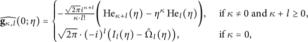 $$\begin{align*}\widehat{\mathbf{g}_{\kappa,l}}(0;\eta)=\begin{cases} -\frac{\sqrt{2\pi}i^{\kappa+l}}{\kappa \cdot l!}\bigg(\operatorname{He}_{\kappa+l}(\eta)-\eta^{\kappa}\operatorname{He}_{l}(\eta)\bigg),& \text{ if }\kappa\neq0\text{ and }\kappa+l\geq0, \\ \sqrt{2\pi}\cdot(-i)^{l}\big(I_{l}(\eta)-\tilde{\Omega}_{l}(\eta)\big),& \text{ if }\kappa=0, \end{cases}\end{align*}$$
where $I_{\nu ,j}$
and
$I_{\nu ,j}$
and $\tilde {\Omega }_{k}$
are defined in equation (3.26) and Remark 3.13, respectively.
$\tilde {\Omega }_{k}$
are defined in equation (3.26) and Remark 3.13, respectively.
Proof When $\kappa \neq 0$
and
$\kappa \neq 0$
and $\eta>0$
, we can integrate equation (3.25) (using the fact that Remark 3.15 extends to the functions
$\eta>0$
, we can integrate equation (3.25) (using the fact that Remark 3.15 extends to the functions $\mathbf {g}_{\kappa ,l}$
) to obtain
$\mathbf {g}_{\kappa ,l}$
) to obtain
 $$ \begin{align*} \widehat{\mathbf{g}_{\kappa,l}}(0;\eta)&=\int_{-\infty}^{\infty}\mathbf{g}_{\kappa,l}(\xi;\eta)d\xi=\frac{1}{\kappa}\int_{-\infty}^{\infty} \bigg(\kern-2pt -\frac{\mathrm{g}_{\kappa+l+1}(\xi;\eta)}{l!}+\sqrt{2\pi}(i\eta)^{\kappa}P_{l}(i\eta)\delta(\xi)\bigg)d\xi \\ &=\frac{1}{\kappa}\bigg(-\frac{\widehat{\mathrm{g}_{\kappa+l+1}}(0;\eta)}{l!}+\sqrt{2\pi}P_{l}(i\eta)(i\eta)^{\kappa}\kern-1pt\bigg), \end{align*} $$
which gives the desired value by Lemma 3.19 and Corollary 3.7.
When $\kappa =0$
, we evaluate directly, where the formula from Remark 3.20 gives
$\kappa =0$
, we evaluate directly, where the formula from Remark 3.20 gives
 $$\begin{align*}\widehat{\mathbf{g}_{0,l}}(0;\eta)=\sqrt{2\pi}(-i)^{l}I_{l}(\eta)-(-1)^{l}\int_{-\infty}^{\infty}\frac{h_{l}(\xi)-(-1)^{l}(P_{l}(i\eta)\mathrm{e}(\xi)+\Pi_{l}(\xi,i\eta)\mathrm{g}(\xi))}{\xi+i\eta}d\xi.\end{align*}$$
As equation (3.17) transforms the latter integral into $(-1)^{l}\sqrt {2\pi }\Omega _{l}(i\eta )$
via equation (3.15), we get the desired value by Remark 3.13. This proves the proposition.
$(-1)^{l}\sqrt {2\pi }\Omega _{l}(i\eta )$
via equation (3.15), we get the desired value by Remark 3.13. This proves the proposition.
3.6 Asymptotic estimates
For determining the asymptotic behavior of the functions $I_{\nu ,j}$
and the Fourier transforms
$I_{\nu ,j}$
and the Fourier transforms $\widehat {\mathbf {g}_{\kappa ,l}}$
, we shall also need the following special functions. Like the definition of
$\widehat {\mathbf {g}_{\kappa ,l}}$
, we shall also need the following special functions. Like the definition of $\tilde {\Omega }_{k}$
in Remark 3.13, the polynomials
$\tilde {\Omega }_{k}$
in Remark 3.13, the polynomials $P_{\nu }$
and
$P_{\nu }$
and $Q_{\nu }$
for
$Q_{\nu }$
for $\nu \in \mathbb {Z}$
given in equation (3.6) and Remark 3.8 have the modifications
$\nu \in \mathbb {Z}$
given in equation (3.6) and Remark 3.8 have the modifications
 $$ \begin{align} \widetilde{P}_{\nu}(\eta):=i^{\nu}P_{\nu}(i\eta)\qquad\mathrm{and}\qquad\widetilde{Q}_{\nu}(\eta):=i^{\nu-1}Q_{\nu}(i\eta), \end{align} $$
of the same parities as $P_{\nu }$
and
$P_{\nu }$
and $Q_{\nu }$
. Using these, we define the functions
$Q_{\nu }$
. Using these, we define the functions
 $$ \begin{align} \begin{aligned} &J_{-1}(\eta):=\mathrm{g}(i\eta)=e^{\eta^{2}/2},\quad J_{0}(\eta):=-\int_{0}^{\eta}e^{r^{2}/2}dr=\frac{1}{\sqrt{2\pi}}\int_{0}^{\infty} \frac{e^{-\eta s}-e^{\eta s}}{s}\mathrm{g}(s)ds, \\ &\mathrm{and}\qquad J_{\nu}(\eta):=\tilde{P}_{\nu}(\eta)J_{0}(\eta)-\tilde{Q}_{\nu}(\eta)J_{-1}(\eta)\qquad\mathrm{for}\qquad\nu\in\mathbb{Z} \end{aligned} \end{align} $$
(the two expressions for $J_{0}(\eta )$
are the same because they vanish at
$J_{0}(\eta )$
are the same because they vanish at $\eta =0$
and have the same derivative, and since
$\eta =0$
and have the same derivative, and since $\widetilde {P}_{0}=\widetilde {Q}_{-1}=1$
and
$\widetilde {P}_{0}=\widetilde {Q}_{-1}=1$
and $\widetilde {P}_{-1}=\widetilde {Q}_{0}=0$
, the two definitions for
$\widetilde {P}_{-1}=\widetilde {Q}_{0}=0$
, the two definitions for $\nu =0$
and for
$\nu =0$
and for $\nu =-1$
coincide). Since the polynomials from equation (3.30) satisfy identities analogous to those from equation (3.6) and Remark 3.6, the latter of which yields the equality
$\nu =-1$
coincide). Since the polynomials from equation (3.30) satisfy identities analogous to those from equation (3.6) and Remark 3.6, the latter of which yields the equality $\eta J_{\nu }(\eta )+\eta J_{\nu -1}(\eta )=-J_{\nu -2}(\eta )$
for every
$\eta J_{\nu }(\eta )+\eta J_{\nu -1}(\eta )=-J_{\nu -2}(\eta )$
for every $\eta $
and
$\eta $
and $\nu $
, evaluating the derivatives of
$\nu $
, evaluating the derivatives of $J_{0}$
and
$J_{0}$
and $J_{-1}$
implies, for all
$J_{-1}$
implies, for all $\nu \in \mathbb {Z}$
, the relations
$\nu \in \mathbb {Z}$
, the relations
 $$ \begin{align} J_{\nu}'=-J_{\nu-1},\quad J_{\nu}(-\eta)=(-1)^{\nu-1}J_{\nu}(\eta),\quad\mathrm{and}\quad\eta^{3}\frac{d}{d\eta}\frac{J_{\nu}(\eta)}{\eta^{\nu}}=\frac{J_{\nu-2}(\eta)}{\eta^{\nu-2}}. \end{align} $$
The following estimates will be helpful when we evaluate sums of Fourier transforms later.
Lemma 3.23 For any $\epsilon>0$
and fixed
$\epsilon>0$
and fixed $\eta \in \mathbb {R}$
, we have the asymptotic growth
$\eta \in \mathbb {R}$
, we have the asymptotic growth
 $$\begin{align*}I_{-1,0}(\eta,t)=\begin{cases} \sqrt{2\pi}J_{-1}(\eta)+o_{\eta,\epsilon}(e^{-(1-\epsilon)t^{2}/2}), & t\to\infty, \\ o_{\eta,\epsilon}(e^{-(1-\epsilon)t^{2}/2}),& t\to-\infty,\end{cases}\end{align*}$$
with $J_{-1}(\eta )$
from equation (3.31). More generally, given
$J_{-1}(\eta )$
from equation (3.31). More generally, given $j\in \mathbb {N}$
, we have
$j\in \mathbb {N}$
, we have
 $$\begin{align*}I_{-1,j}(\eta,t)=P_{j}(t-\eta)I_{-1,0}(\eta,t)+o_{j,\eta,\epsilon}(e^{-(1-\epsilon)t^{2}/2})\qquad\mathrm{as}\qquad t\to\pm\infty.\end{align*}$$
Moreover, given $\eta>0$
and such
$\eta>0$
and such $\epsilon $
, and with
$\epsilon $
, and with $J_{0}$
from equation (3.31), we get
$J_{0}$
from equation (3.31), we get
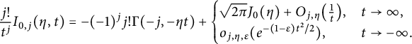 $$\begin{align*}\frac{j!}{t^{j}}I_{0,j}(\eta,t)=-(-1)^{j}j!\Gamma(-j,-\eta t)+\begin{cases} \sqrt{2\pi}J_{0}(\eta)+O_{j,\eta}\big(\frac{1}{t}\big), & t\to\infty, \\ o_{j,\eta,\epsilon}(e^{-(1-\epsilon)t^{2}/2}), & t\to-\infty. \end{cases}\end{align*}$$
Proof Using equation (3.4) and the value $\sqrt {2\pi }$
of
$\sqrt {2\pi }$
of $\int _{-\infty }^{\infty }g(\xi )d\xi $
, the first equation follows from
$\int _{-\infty }^{\infty }g(\xi )d\xi $
, the first equation follows from
 $$\begin{align*}I_{-1,0}(\eta,t)=\int_{-t}^{\infty}e^{-\eta w-w^{2}/2}dw=e^{\eta^{2}/2}\int_{\eta-t}^{\infty} \mathrm{g}(s)ds=\begin{cases}e^{\eta^{2}/2}\big(\sqrt{2\pi}-\mathrm{e}(t-\eta)\big), & t>\eta, \\ -e^{\eta^{2}/2}\mathrm{e}(\eta-t), & t<\eta,\end{cases} \end{align*}$$
and Remark 3.15. Next, using the definition in equation (3.26) and simple algebra, we get, for every $\eta \in \mathbb {R}$
and
$\eta \in \mathbb {R}$
and $j\in \mathbb {N}$
, the equality
$j\in \mathbb {N}$
, the equality
 $$\begin{align*}\delta_{j,0}e^{\eta t-t^{2}/2}=-\int_{-t}^{\infty}\frac{d}{dw}\big(\tfrac{(w+t)^{j}}{j!}e^{-\eta w-w^{2}/2}\big)dw=(j+1)I_{-1,j+1}-(t-\eta)I_{-1,j}-(1-\delta_{j,0})I_{-1,j-1}. \end{align*}$$
Since the left-hand side times any polynomial is $o_{\epsilon }(e^{-(1-\epsilon )t^{2}/2})$
as
$o_{\epsilon }(e^{-(1-\epsilon )t^{2}/2})$
as $t\to \pm \infty $
, a simple induction on j combines with Remark 3.6 to prove the second relation.
$t\to \pm \infty $
, a simple induction on j combines with Remark 3.6 to prove the second relation.
Now, suppose $t\neq 0$
and
$t\neq 0$
and $\eta>0$
. For
$\eta>0$
. For $j=0$
, we evaluate
$j=0$
, we evaluate
 $$\begin{align*}I_{0,0}(\eta,t)=\int_{-t}^{\infty}e^{-\eta w}\frac{\mathrm{g}(w)-1}{w}dw=\int_{-t}^{|t|}e^{-\eta w}\frac{\mathrm{g}(w)}{w}dw+\int_{|t|}^{\infty}e^{-\eta w}\frac{\mathrm{g}(w)}{w}dw-\Gamma(0,-\eta t). \end{align*}$$
As $t\to -\infty $
, the first term above vanishes and the second term is
$t\to -\infty $
, the first term above vanishes and the second term is $o_{\eta ,\epsilon }(e^{-(1-\epsilon )t^{2}/2})$
for any fixed
$o_{\eta ,\epsilon }(e^{-(1-\epsilon )t^{2}/2})$
for any fixed $\eta \in \mathbb {R}$
. As
$\eta \in \mathbb {R}$
. As $t\to \infty $
, the second term behaves the same, whereas using equation (3.31), we see that the first term contributes
$t\to \infty $
, the second term behaves the same, whereas using equation (3.31), we see that the first term contributes
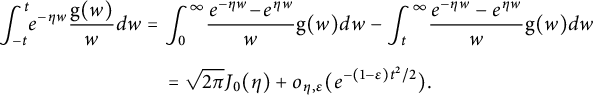 $$\begin{align*}\int_{-t}^{t}\!\!e^{-\eta w}\frac{\mathrm{g}(w)}{w}dw&=\int_{0}^{\infty}\!\frac{e^{-\eta w}\!-\!e^{\eta w}}{w}\mathrm{g}(w)dw-\int_{t}^{\infty}\!\frac{e^{-\eta w}-e^{\eta w}}{w}\mathrm{g}(w)dw\\[6pt] & \quad =\sqrt{2\pi}J_{0}(\eta)+o_{\eta,\epsilon}(e^{-(1-\epsilon)t^{2}/2}). \end{align*}$$
This proves the third equality for $j=0$
. When
$j=0$
. When $j\geq 1$
, we can write
$j\geq 1$
, we can write $\frac {j!}{t^{j}}I_{0,j}(\eta ,t)$
as
$\frac {j!}{t^{j}}I_{0,j}(\eta ,t)$
as
 $$\begin{align*}\frac{1}{t^{j}}\int_{-t}^{\infty}\frac{(w+t)^{j}-t^{j}}{w}e^{-\eta w-w^{2}/2}dw-\frac{e^{\eta t}}{t^{j}}\int_{0}^{\infty}\frac{s^{j}-t^{j}}{s-t}e^{-\eta s}ds+\int_{-t}^{\infty}e^{-\eta w}\frac{\mathrm{g}(w)-1}{w}dw. \end{align*}$$
After expanding $(w+t)^{j}$
binomially, the first term is seen to be
$(w+t)^{j}$
binomially, the first term is seen to be $o_{j,\eta ,\epsilon }(e^{-(1-\epsilon )t^{2}/2})$
as
$o_{j,\eta ,\epsilon }(e^{-(1-\epsilon )t^{2}/2})$
as $t\to -\infty $
and
$t\to -\infty $
and $O_{j,\eta }\big (\frac {1}{t}\big )$
as
$O_{j,\eta }\big (\frac {1}{t}\big )$
as $t\to \infty $
. Expanding
$t\to \infty $
. Expanding $\frac {s^{j}-s^{j}}{s-t}$
and applying equation (3.2), the second term becomes
$\frac {s^{j}-s^{j}}{s-t}$
and applying equation (3.2), the second term becomes $-(-1)^{j}j!\Gamma (-j,-\eta t)+\Gamma (0,-\eta t)$
, and the third term is just the expression for
$-(-1)^{j}j!\Gamma (-j,-\eta t)+\Gamma (0,-\eta t)$
, and the third term is just the expression for $j=0$
. Putting everything together proves the last desired equality. This proves the lemma.
$j=0$
. Putting everything together proves the last desired equality. This proves the lemma.
In fact, the first term in the last equation in the proof of Lemma 3.23 can easily be evaluated explicitly up to $o_{j,\eta ,\epsilon }(e^{-(1-\epsilon )t^{2}/2})$
also when
$o_{j,\eta ,\epsilon }(e^{-(1-\epsilon )t^{2}/2})$
also when $t\to \infty $
, but the estimate
$t\to \infty $
, but the estimate $O_{j,\eta }\big (\frac {1}{t}\big )$
will be sufficient for our purposes.
$O_{j,\eta }\big (\frac {1}{t}\big )$
will be sufficient for our purposes.
Remark 3.24 The generating series $\sum _{j=0}^{\infty }I_{-1,j}(0,0)X^{j}$
of the constants
$\sum _{j=0}^{\infty }I_{-1,j}(0,0)X^{j}$
of the constants $\big \{I_{-1,j}(0,0)\}_{j=0}^{\infty }$
is
$\big \{I_{-1,j}(0,0)\}_{j=0}^{\infty }$
is
 $$\begin{align*}\int_{0}^{\infty}e^{wX-w^{2}/2}dw=e^{X^{2}/2}\int_{0}^{\infty}e^{-(w-X)^{2}/2}dw=e^{X^{2}/2} \bigg(\int_{0}^{\infty}e^{-w^{2}/2}dw+\int_{0}^{X}e^{-w^{2}/2}dw\bigg) \end{align*}$$
(by symmetry), which equals $\Upsilon (0,X)+\sqrt {\pi /2}\Psi (0,X)$
by Theorem 3.4. It therefore follows from equations (3.7) and (3.17) and the parity from Proposition 3.14 that
$\Upsilon (0,X)+\sqrt {\pi /2}\Psi (0,X)$
by Theorem 3.4. It therefore follows from equations (3.7) and (3.17) and the parity from Proposition 3.14 that
 $$\begin{align*}I_{-1,j}(0,0)=Q_{j}(0)+\sqrt{\pi/2}P_{j}(0)=\lim_{\xi\to0^{-}}h_{j}(\xi)=(-1)^{j-1}\lim_{\xi\to0^{+}}h_{j}(\xi)\quad\mathrm{for}\quad j\in\mathbb{N}. \end{align*}$$
We can now state the asymptotic expansion of $\widehat {\mathbf {g}_{\kappa ,l}}(t;\eta )$
.
$\widehat {\mathbf {g}_{\kappa ,l}}(t;\eta )$
.
Proposition 3.25 Take $\kappa \in \mathbb {Z}$
,
$\kappa \in \mathbb {Z}$
, $l\in \mathbb {N}$
, and
$l\in \mathbb {N}$
, and $\eta \in \mathbb {R}$
, with
$\eta \in \mathbb {R}$
, with $\eta>0$
in case
$\eta>0$
in case $\kappa \leq 0$
. We then have
$\kappa \leq 0$
. We then have
 $$\begin{align*}\widehat{\mathbf{g}_{\kappa,l}}(t;\eta)=-\sqrt{2\pi}\frac{i^{\kappa+l}\operatorname{He}_{l}(\eta)}{l!(-2\pi t)^{\kappa}}e^{-2\pi\eta t}\Gamma(\kappa,-2\pi\eta t)+o_{\kappa,l,\eta,\epsilon}(e^{-2\pi^{2}(1-\epsilon)t^{2}}), \end{align*}$$
an expression holding as $t\to -\infty $
as well as in the limit
$t\to -\infty $
as well as in the limit $t\to \infty $
when
$t\to \infty $
when $\kappa \geq 1$
. On the other hand, if
$\kappa \geq 1$
. On the other hand, if $\kappa \leq 0$
and
$\kappa \leq 0$
and $\eta>0$
, then the limit as
$\eta>0$
, then the limit as $t\to \infty $
is given by the same formula plus the term
$t\to \infty $
is given by the same formula plus the term
 $$\begin{align*}\frac{2\pi(-i)^{\kappa+l}}{|\kappa|!(-2\pi t)^{\kappa}}e^{-2\pi\eta t}\big[J_{l}(\eta)+O_{\kappa,l,\eta}\big(\tfrac{1}{t}\big)\big],\end{align*}$$
where $J_{l}(\eta )$
is the function defined in equation (3.31).
$J_{l}(\eta )$
is the function defined in equation (3.31).
Proof Taking the Fourier transform of equation (3.24) allows us to write
 $$\begin{align*}\widehat{\mathbf{g}_{\kappa,l}}(t;\eta)=P_{l}(i\eta)\widehat{\mathrm{e}_{\kappa}}(t;\eta)+\Pi_{l}\big(\tfrac{\partial_{t}}{-2\pi i},i\eta\big)\widehat{\mathrm{g}_{\kappa}}(t;\eta). \end{align*}$$
When $\kappa \geq 1$
, we apply Lemma 3.19 and equation (3.2) to obtain that
$\kappa \geq 1$
, we apply Lemma 3.19 and equation (3.2) to obtain that
 $$\begin{align*}\widehat{\mathrm{e}_{\kappa}}(t;\eta)=-\sqrt{2\pi}\frac{e^{-2\pi\eta t}\Gamma(\kappa,-2\pi\eta t)}{(2\pi it)^{\kappa}}+o_{\kappa,l,\epsilon}(\eta^{\kappa-1}e^{-(1-\epsilon)t^{2}/2})\qquad\mathrm{as}\qquad t\to\pm\infty \end{align*}$$
and that $\Pi _{l}\big (\frac {\partial _{t}}{-2\pi i},i\eta \big )\widehat {\mathrm {g}_{\kappa }}(t;\eta )$
is bounded by the same error term. This establishes, via Corollary 3.7, the desired formula in this case. On the other hand, for
$\Pi _{l}\big (\frac {\partial _{t}}{-2\pi i},i\eta \big )\widehat {\mathrm {g}_{\kappa }}(t;\eta )$
is bounded by the same error term. This establishes, via Corollary 3.7, the desired formula in this case. On the other hand, for $\kappa \leq 0$
and
$\kappa \leq 0$
and $\eta>0$
, we deduce from Lemma 3.19 that
$\eta>0$
, we deduce from Lemma 3.19 that
 $$\begin{align*}\widehat{\mathbf{g}_{\kappa,l}}(t;\eta)&=\sqrt{2\pi} \cdot i^{\kappa}e^{-2\pi\eta t}P_{l}(i\eta)I_{0,-\kappa}(\eta,2\pi t)\\& \quad +\sqrt{2\pi} \cdot i^{\kappa-1}\Pi_{l}\big(\tfrac{\partial_{t}}{-2\pi i},i\eta\big)e^{-2\pi\eta t}I_{-1,-\kappa}(\eta,2\pi t).\end{align*}$$
Lemma 3.23 now shows that, in the limit $t\to -\infty $
, the first summand is
$t\to -\infty $
, the first summand is
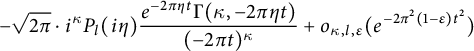 $$\begin{align*}-\sqrt{2\pi} \cdot i^{\kappa}P_{l}(i\eta)\frac{e^{-2 \pi\eta t}\Gamma(\kappa,-2\pi\eta t)}{(-2\pi t)^{\kappa}}+o_{\kappa,l,\epsilon}(e^{-2\pi^{2}(1-\epsilon)t^{2}}) \end{align*}$$
and the second one goes into the error term, which yields the required formula also here by another application of Corollary 3.7. In the limit $t\to \infty $
, we get the same contribution, but we need to consider the additional terms from Lemma 3.23 in that limit. The term arising from the first summand is
$t\to \infty $
, we get the same contribution, but we need to consider the additional terms from Lemma 3.23 in that limit. The term arising from the first summand is
 $$ \begin{align} \frac{2\pi \cdot i^{\kappa}e^{-2\pi\eta t}}{|\kappa|!(2\pi t)^{\kappa}}\big[P_{l}(i\eta)J_{0}(\eta)+O_{\kappa,l,\eta}\big(\tfrac{1}{t}\big)\big]. \end{align} $$
For the one from the second summand, Remark 3.10 allows us to write
 $$ \begin{align*} &\Pi_{l}\big(\tfrac{\partial_{t}}{-2\pi i},i\eta\big)e^{-2\pi\eta t}I_{-1,-\kappa}(\eta,2\pi t)\\ & \quad =\big[-Q_{l}(i\eta)+\tilde{\Pi}_{l}\big(\tfrac{\partial_{t}}{-2\pi i}+i\eta,i\eta\big)\big]e^{-2\pi\eta t}I_{-1,-\kappa}(\eta,2\pi t) \\ & \quad =e^{-2\pi\eta t}\big[-Q_{l}(i\eta)I_{-1,-\kappa}(\eta,2\pi t)+\tilde{\Pi}_{l}\big(\tfrac{\partial_{t}}{-2\pi i},i\eta\big)I_{-1,-\kappa}(\eta,2\pi t)\big] \end{align*} $$
(by the action on that exponent). Lemma 3.23 and the fact that Corollary 3.2 gives the estimate $P_{|\kappa |}(2\pi t-\eta )=\frac {(2\pi t)^{|\kappa |}}{|\kappa |!}\big [1+O_{\kappa ,\eta }\big (\frac {1}{t}\big )\big ]$
show that
$P_{|\kappa |}(2\pi t-\eta )=\frac {(2\pi t)^{|\kappa |}}{|\kappa |!}\big [1+O_{\kappa ,\eta }\big (\frac {1}{t}\big )\big ]$
show that $\sqrt {2\pi } \cdot i^{\kappa -1}$
times the first summand here is
$\sqrt {2\pi } \cdot i^{\kappa -1}$
times the first summand here is
 $$\begin{align*}-\frac{2\pi \cdot i^{\kappa-1}e^{-2\pi\eta t}}{|\kappa|!(2\pi t)^{\kappa}}\big[Q_{l}(i\eta)J_{-1}(\eta)+O_{\kappa,l,\eta}\big(\tfrac{1}{t}\big)\big]. \end{align*}$$
Equations (3.30) and (3.31) now show that this expression combines with the one from equation (3.33) to the asserted extra term, up to the required error term. Finally, equation (3.28) and the property of $\tilde {\Pi }_{l}$
from Remark 3.10 imply, via Lemma 3.23 again, that the expression involving that polynomial also goes into the error term. This proves the proposition.
$\tilde {\Pi }_{l}$
from Remark 3.10 imply, via Lemma 3.23 again, that the expression involving that polynomial also goes into the error term. This proves the proposition.
3.7 Lattice sums
To evaluate the constant term of the Shintani lift, we need to calculate certain lattice sums involving the function $\mathbf {g}_{\kappa ,l}$
defined in equation (3.24). For
$\mathbf {g}_{\kappa ,l}$
defined in equation (3.24). For $\kappa \in \mathbb {Z}$
,
$\kappa \in \mathbb {Z}$
, $l\in \mathbb {N}$
,
$l\in \mathbb {N}$
, $\eta \in \mathbb {R}$
, a real number
$\eta \in \mathbb {R}$
, a real number $\upsilon>0$
, and an element
$\upsilon>0$
, and an element $\omega \in \mathbb {R}/\mathbb {Z}$
, we consider the sum
$\omega \in \mathbb {R}/\mathbb {Z}$
, we consider the sum
 $$ \begin{align} \mathbf{G}_{\kappa,l}(\omega;\upsilon,\eta):=\sum_{0\neq\xi\in\mathbb{Z}+\omega}\mathbf{g}_{\kappa,l}(\upsilon\xi;\eta), \end{align} $$
which converges absolutely by Remark 3.15 and defines a continuous function in $\eta $
. We will be interested in its value at
$\eta $
. We will be interested in its value at $\eta =0$
, denoted by
$\eta =0$
, denoted by
 $$ \begin{align} \mathbf{G}_{\kappa,l}(\omega;\upsilon):=\mathbf{G}_{\kappa,l}(\omega;\upsilon,0)=\lim_{\eta\to0^{+}}\mathbf{G}_{\kappa,l}(\omega;\upsilon,\eta), \end{align} $$
and its asymptotic expansion as $\upsilon \to 0^{+}$
.
$\upsilon \to 0^{+}$
.
Remark 3.26 The function $\mathbf {G}_{\kappa ,l}$
from equation (3.34), or its variant from equation (3.35), is defined as a lattice sum, and would naturally be expressible also via its Fourier series, which amounts to the Poisson Summation Formula. Indeed, the summed function
$\mathbf {G}_{\kappa ,l}$
from equation (3.34), or its variant from equation (3.35), is defined as a lattice sum, and would naturally be expressible also via its Fourier series, which amounts to the Poisson Summation Formula. Indeed, the summed function $\mathbf {g}_{\kappa ,l}$
is differentiable away from 0 with a strongly decaying derivative, making
$\mathbf {g}_{\kappa ,l}$
is differentiable away from 0 with a strongly decaying derivative, making $\mathbf {G}_{\kappa ,l}$
differentiable with respect to
$\mathbf {G}_{\kappa ,l}$
differentiable with respect to $\omega $
when
$\omega $
when $\omega \neq 0$
. Therefore, the Fourier expansion of the lattice sum
$\omega \neq 0$
. Therefore, the Fourier expansion of the lattice sum $\mathbf {G}_{\kappa ,l}$
converges pointwise to it for every
$\mathbf {G}_{\kappa ,l}$
converges pointwise to it for every $\omega \neq 0$
. Since the mth Fourier coefficient of
$\omega \neq 0$
. Since the mth Fourier coefficient of $\mathbf {G}_{\kappa ,l}$
(for
$\mathbf {G}_{\kappa ,l}$
(for $\eta \neq 0$
) is, by simple integration,
$\eta \neq 0$
) is, by simple integration, $\frac {1}{\upsilon }\widehat {\mathbf {g}_{\kappa ,l}}\big (\frac {m}{\upsilon };\eta \big )$
, we obtain that the Poisson Summation Formula for
$\frac {1}{\upsilon }\widehat {\mathbf {g}_{\kappa ,l}}\big (\frac {m}{\upsilon };\eta \big )$
, we obtain that the Poisson Summation Formula for $\mathbf {G}_{\kappa ,l}$
is valid for
$\mathbf {G}_{\kappa ,l}$
is valid for $\omega \neq 0$
. In fact, since the one-sided derivatives of
$\omega \neq 0$
. In fact, since the one-sided derivatives of $\mathbf {g}_{\kappa ,l}$
also exist (provided that
$\mathbf {g}_{\kappa ,l}$
also exist (provided that $\mathbf {g}_{\kappa ,l}(0)$
is modified to have the limit value from the appropriate side), the Fourier series converges also at
$\mathbf {g}_{\kappa ,l}(0)$
is modified to have the limit value from the appropriate side), the Fourier series converges also at $\omega =0$
to a value that can be described (both Fourier series convergence statements follow, for example, from the Dirichlet–Dini Criterion). However, it is easier to consider the value at
$\omega =0$
to a value that can be described (both Fourier series convergence statements follow, for example, from the Dirichlet–Dini Criterion). However, it is easier to consider the value at $\omega =0$
in terms of equation (3.44).
$\omega =0$
in terms of equation (3.44).
For analyzing it, we first need to recall a few familiar functions. Let $\{B_{\mu }(\omega )\}_{\mu =0}^{\infty }$
(for
$\{B_{\mu }(\omega )\}_{\mu =0}^{\infty }$
(for $\omega \in \mathbb {R}$
) be the Bernoulli polynomials defined as
$\omega \in \mathbb {R}$
) be the Bernoulli polynomials defined as
 $$\begin{align*}\frac{te^{\omega t}}{e^{t}-1}=\sum_{\mu=0}^{\infty}B_{\mu}(\omega)\frac{t^{\mu}}{\mu!},\quad\mathrm{so\ that\ in\ particular}\quad B_{1}(\omega)=\omega-\tfrac{1}{2}, \end{align*}$$
and then $B_{\mu }:=B_{\mu }(0)$
are the Bernoulli numbers. Moreover, one defines
$B_{\mu }:=B_{\mu }(0)$
are the Bernoulli numbers. Moreover, one defines $\mathbb {B}_{\mu }$
to be the 1-periodic function that coincides with
$\mathbb {B}_{\mu }$
to be the 1-periodic function that coincides with $B_{\mu }$
on the interval
$B_{\mu }$
on the interval $(0,1)$
, and whose value on the integers is 0 in case
$(0,1)$
, and whose value on the integers is 0 in case $\mu =1$
and
$\mu =1$
and $B_{\mu }$
otherwise. Then
$B_{\mu }$
otherwise. Then $\mathbb {B}_{\mu }$
with
$\mathbb {B}_{\mu }$
with $\mu \geq 2$
is continuous on
$\mu \geq 2$
is continuous on $\mathbb {R}$
(and
$\mathbb {R}$
(and $\mathbb {B}_{0}$
is the constant function 1), and we have
$\mathbb {B}_{0}$
is the constant function 1), and we have
 $$ \begin{align} \mathbb{B}_{1}(0)=0=\lim_{\omega\to0^{+}}\mathbb{B}_{1}(\omega)+\tfrac{1}{2}=\lim_{\omega\to0-}\mathbb{B}_{1}(\omega)-\tfrac{1}{2}\quad\mathrm{and}\quad\mathbb{B}_{\mu}(\omega)=-\sum_{0 \neq m\in\mathbb{Z}}\frac{\mu!\mathbf{e}(m\omega)}{(2\pi im)^{\mu}}, \end{align} $$
the latter Fourier expansion being valid for every $\omega \in \mathbb {R}/\mathbb {Z}$
and
$\omega \in \mathbb {R}/\mathbb {Z}$
and $0<\mu \in \mathbb {N}$
(this is essentially equations (13)–(15) in Section 1.13 of [Reference Erdélyi, Magnus, Oberhettinger and TricomiEMOT]).
$0<\mu \in \mathbb {N}$
(this is essentially equations (13)–(15) in Section 1.13 of [Reference Erdélyi, Magnus, Oberhettinger and TricomiEMOT]).
We also recall from Section 1.11 of [Reference Erdélyi, Magnus, Oberhettinger and TricomiEMOT] the function
 $$ \begin{align} F(q,s)=\sum_{m=1}^{\infty}\frac{q^{m}}{m^{s}}\qquad\mathrm{for}\qquad s\in\mathbb{C} \quad\mathrm{and}\quad q\in\mathbb{C}\quad\mathrm{with}\quad|q|<1. \end{align} $$
Since we shall use this function only when $s=-j$
for
$s=-j$
for $j\in \mathbb {N}$
, where
$j\in \mathbb {N}$
, where $F(q,-j)$
is a polynomial in q divided by
$F(q,-j)$
is a polynomial in q divided by $(1-q)^{j+1}$
, the analytic continuation to any
$(1-q)^{j+1}$
, the analytic continuation to any $q\in \mathbb {C}\setminus [1,\infty )$
, and even to any
$q\in \mathbb {C}\setminus [1,\infty )$
, and even to any $1 \neq q\in \mathbb {C}$
, is immediate. Writing
$1 \neq q\in \mathbb {C}$
, is immediate. Writing $q=\mathbf {e}(\omega )$
for
$q=\mathbf {e}(\omega )$
for $\omega \in \mathbb {R}$
, the fact that
$\omega \in \mathbb {R}$
, the fact that $F(q,0)=\frac {q}{1-q}$
combines with equation (15) of Section 1.11 of [Reference Erdélyi, Magnus, Oberhettinger and TricomiEMOT] (for
$F(q,0)=\frac {q}{1-q}$
combines with equation (15) of Section 1.11 of [Reference Erdélyi, Magnus, Oberhettinger and TricomiEMOT] (for $j\geq 1$
) to give, for all
$j\geq 1$
) to give, for all $j\in \mathbb {N}$
, the expansion
$j\in \mathbb {N}$
, the expansion
 $$ \begin{align} F\big(\mathbf{e}(\omega),-j\big)=\frac{j!}{(-2\pi i\cdot\omega)^{j+1}}-\frac{B_{j+1}+\delta_{j,0}}{j+1}+O(\omega). \end{align} $$
Another function to recall is the polygamma function, defined for $m\in \mathbb {N}$
and
$m\in \mathbb {N}$
and $z\in \mathbb {C}$
as
$z\in \mathbb {C}$
as
 $$ \begin{align} \psi^{(m)}(z):=\frac{d^{m+1}}{dz^{m+1}}\log\Gamma(z)=-\gamma\delta_{m,0}+(-1)^{m}m!\sum_{a=0}^{\infty}\bigg(\frac{\delta_{m,0}}{(a+1)^{m+1}}-\frac{1}{(a+z)^{m+1}}\bigg), \end{align} $$
where $\delta _{m,0}$
is the Kronecker
$\delta _{m,0}$
is the Kronecker $\delta $
-symbol again.
$\delta $
-symbol again.
Let $\tilde {\psi }^{(m)}$
be the 1-periodic function that coincides with
$\tilde {\psi }^{(m)}$
be the 1-periodic function that coincides with $\psi ^{(m)}$
from equation (3.39) on
$\psi ^{(m)}$
from equation (3.39) on $(0,1]$
. Then, for
$(0,1]$
. Then, for $\kappa \in \mathbb {Z}$
and
$\kappa \in \mathbb {Z}$
and $\omega \in \mathbb {R}/\mathbb {Z}$
, we define
$\omega \in \mathbb {R}/\mathbb {Z}$
, we define
 $$ \begin{align} \Phi_{\kappa}(\omega):=\begin{cases} -\mathbb{B}_{\kappa}(\omega)/\kappa, & \kappa\geq1, \\ -\big[\tilde{\psi}^{(|\kappa|)}(-\omega)+(-1)^{\kappa}\tilde{\psi}^{(|\kappa|)}(\omega)\big]\big/2|\kappa|!, & \kappa\leq0, \end{cases} \end{align} $$
as well as
 $$ \begin{align} \Xi_{\kappa}(\omega):=\frac{(-2\pi i)^{1-\kappa}}{\sqrt{2\pi}}\begin{cases} F(\mathbf{e}(\omega),\kappa)/|\kappa|!+\delta_{\kappa,0}/2, & \kappa\leq0\text{ and }\omega\not\in\mathbb{Z}, \\ -\mathbb{B}_{1-\kappa}(0)/(1-\kappa)!, & \kappa\leq1\text{ and }\omega\in\mathbb{Z}, \\ 0, & \text{otherwise.} \end{cases} \end{align} $$
Note that, for all $\kappa \in 2\mathbb {Z}$
, we have the equality
$\kappa \in 2\mathbb {Z}$
, we have the equality
 $$ \begin{align} \Phi_{\kappa}(1)=\operatorname{CT}_{s=1-\kappa}\zeta(s). \end{align} $$
Recalling the notation $H_{n}$
for the nth harmonic number, we shall also need the constant
$H_{n}$
for the nth harmonic number, we shall also need the constant
 $$ \begin{align} C_{l}:=\frac{\gamma+\log2-2H_{l}+H_{\lfloor l/2 \rfloor}}{2}=\frac{\gamma+\log2}{2}-\sum_{a=1,\ 2 \nmid a}^{l}\frac{1}{a}. \end{align} $$
We remark that it is easy to see, via the asymptotic $H_{n}=\log n+\gamma +o(1)$
as
$H_{n}=\log n+\gamma +o(1)$
as $n\to \infty $
, that
$n\to \infty $
, that $C_{l}$
from equation (3.43) grows as
$C_{l}$
from equation (3.43) grows as $-\frac {\log l}{2}+o(1)$
as
$-\frac {\log l}{2}+o(1)$
as $l\to \infty $
.
$l\to \infty $
.
The evaluation of the expression that we need is now carried out as follows.
Proposition 3.27 Take $\kappa \in \mathbb {Z}$
,
$\kappa \in \mathbb {Z}$
, $l\in \mathbb {N}$
,
$l\in \mathbb {N}$
, $\eta \in \mathbb {R}$
,
$\eta \in \mathbb {R}$
, $\upsilon>0$
, and
$\upsilon>0$
, and $\omega \in \mathbb {R}/\mathbb {Z}$
. Then the value of the expression
$\omega \in \mathbb {R}/\mathbb {Z}$
. Then the value of the expression $\mathbf {G}_{\kappa ,l}(\omega ;\upsilon )$
from equation (3.35) is
$\mathbf {G}_{\kappa ,l}(\omega ;\upsilon )$
from equation (3.35) is
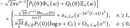 $$\begin{align*}&-\sqrt{2\pi}\upsilon^{\kappa-1}\big[P_{l}(0)\Phi_{\kappa}(\omega)+Q_{l}(0)\Xi_{\kappa}(\omega)\big]\\ & \quad +\begin{cases} -\frac{\sqrt{2\pi} \cdot i^{\kappa+l}\operatorname{He}_{\kappa+l}(0)}{\upsilon\kappa \cdot l!}+o_{\kappa,l,\epsilon}(e^{-2\pi^{2}(1-\epsilon)/\upsilon^{2}}), & \kappa\geq1, \\ \frac{\sqrt{2\pi}}{\upsilon}\delta_{\kappa,0}P_{l}(0)(\log\upsilon+C_{l})+O_{\kappa,l,\omega}(\upsilon^{\kappa}), & \kappa\leq0, \end{cases} \end{align*}$$
with the O-notation concerning the behavior as $\upsilon \to 0^{+}$
.
$\upsilon \to 0^{+}$
.
Proof Consider first the case where $\kappa \geq 1$
. For
$\kappa \geq 1$
. For $\omega \neq 0$
, we use the Poisson Summation Formula (justified by Remark 3.26), and applying Propositions 3.22 and 3.25 gives us
$\omega \neq 0$
, we use the Poisson Summation Formula (justified by Remark 3.26), and applying Propositions 3.22 and 3.25 gives us
 $$ \begin{align*} &\mathbf{G}_{\kappa,l}(\omega;\upsilon)\\ & \quad =\frac{1}{\upsilon}\bigg(\widehat{\mathbf{g}_{\kappa,l}}(0;0)+\lim_{\eta\to0}\sum_{0 \neq m\in\mathbb{Z}}\mathbf{e}(m\omega)\widehat{\mathbf{g}_{\kappa,l}}\big(\tfrac{m}{\upsilon};\eta\big)\bigg) \\ & \quad =-\frac{\sqrt{2\pi}i^{\kappa+l}}{\upsilon\kappa}\bigg(\frac{\operatorname{He}_{\kappa+l}(0)}{l!}+\frac{\kappa\operatorname{He}_{l}(0)}{l!}\lim_{\eta\to0}\sum_{0 \neq m\in\mathbb{Z}}\frac{\mathbf{e}(m\omega)\upsilon^{\kappa}}{(-2\pi m)^{\kappa}}e^{-2\pi\eta m/\upsilon}\Gamma\big(\kappa,-\tfrac{2\pi\eta m}{\upsilon}\big)\bigg) \\ & \quad =\frac{\sqrt{2\pi}}{\upsilon\kappa}\bigg(\frac{-i^{\kappa+l}\operatorname{He}_{\kappa+l}(0)}{l!}-\kappa!P_{l}(0)\sum_{0 \neq m\in\mathbb{Z}}\frac{\mathbf{e}(m\omega)\upsilon^{\kappa}}{(2\pi im)^{\kappa}}\bigg) \\ & \quad =\frac{\sqrt{2\pi}}{\upsilon\kappa}\bigg(\frac{-i^{\kappa+l}\operatorname{He}_{\kappa+l}(0)}{l!}+P_{l}(0)\upsilon^{\kappa}\mathbb{B}_{\kappa}(\omega)\bigg), \end{align*} $$
via Corollary 3.7 and equation (3.36), up to an error term of $o_{\kappa ,l,\epsilon }(e^{-2\pi ^{2}(1-\epsilon )/\upsilon ^{2}})$
. From the definition, it is also clear that
$o_{\kappa ,l,\epsilon }(e^{-2\pi ^{2}(1-\epsilon )/\upsilon ^{2}})$
. From the definition, it is also clear that
 $$ \begin{align} \mathbf{G}_{\kappa,l}(0;\upsilon)=\lim_{\omega\to0^{+}}\big(\mathbf{G}_{\kappa,l}(\omega+\mathbb{Z};\upsilon)-\mathbf{g}_{\kappa,l}(\upsilon\omega;0)\big). \end{align} $$
Equation (3.24) implies that $-\lim _{\xi \to 0}\mathbf {g}_{\kappa ,l}(\xi ;0)$
vanishes for
$-\lim _{\xi \to 0}\mathbf {g}_{\kappa ,l}(\xi ;0)$
vanishes for $\kappa>1$
, and we have
$\kappa>1$
, and we have
 $$\begin{align*}-\lim_{\xi\to0^{+}}\mathbf{g}_{1,l}(\xi;0)=\lim_{\xi\to0^{+}}(-1)^{l+1}h_{l}(\xi)=I_{-1,l}(0,0)=P_{l}(0)\sqrt{\pi/2}+Q_{l}(0) \end{align*}$$
by Remark 3.24. Substituting these into equation (3.44), and applying equation (3.36) for $\kappa =1$
, completes the proof for
$\kappa =1$
, completes the proof for $\kappa \geq 1$
.
$\kappa \geq 1$
.
For $\kappa \leq 0$
, we will first consider the case where
$\kappa \leq 0$
, we will first consider the case where $l=1$
, in which
$l=1$
, in which
 $$\begin{align*}\mathbf{g}_{\kappa,1}(\xi;0)=\xi^{\kappa}h_{0}(\xi)-\xi^{\kappa-1}h_{1}(\xi)=-\xi^{\kappa-1}\mathrm{g}(\xi);\quad\!\!\mathrm{hence}\!\!\quad \mathbf{G}_{\kappa,1}(\omega;\upsilon)=-\lim_{\eta\to0^{+}}\sum_{0 \neq \xi\in\mathbb{Z}+\omega}\mathrm{g_{\kappa}}(\upsilon\xi;\eta). \end{align*}$$
Assuming that $\omega \neq 0$
, we apply equation (3.35), the Poisson summation formula again, Lemmas 3.19 and 3.23, and equations (3.11) and equation (3.37) (with its analytic continuation), which compares
$\omega \neq 0$
, we apply equation (3.35), the Poisson summation formula again, Lemmas 3.19 and 3.23, and equations (3.11) and equation (3.37) (with its analytic continuation), which compares $\mathbf {G}_{\kappa ,1}(\omega ;\upsilon )$
with
$\mathbf {G}_{\kappa ,1}(\omega ;\upsilon )$
with
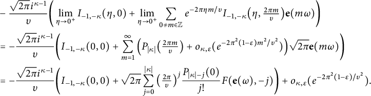 $$ \begin{align} &-\frac{\sqrt{2\pi}i^{\kappa-1}}{\upsilon}\bigg(\lim_{\eta\to0^{+}}I_{-1,-\kappa}(\eta,0)+\lim_{\eta\to0^{+}}\sum_{0 \neq m\in\mathbb{Z}}e^{-2\pi\eta m/\upsilon}I_{-1,-\kappa}\big(\eta,\tfrac{2\pi m}{\upsilon}\big)\mathbf{e}(m\omega)\bigg)\nonumber \\ &=-\frac{\sqrt{2\pi}i^{\kappa-1}}{\upsilon}\bigg(I_{-1,-\kappa}(0,0)+\sum_{m=1}^{\infty}\Big(P_{|\kappa|}\big(\tfrac{2\pi m}{\upsilon}\big)+o_{\kappa,\epsilon}(e^{-2\pi^{2}(1-\epsilon)m^{2}/\upsilon^{2}})\Big)\sqrt{2\pi}\mathbf{e}(m\omega)\bigg) \nonumber\\ &=-\frac{\sqrt{2\pi}i^{\kappa-1}}{\upsilon}\bigg(I_{-1,-\kappa}(0,0)+ \sqrt{2\pi}\sum_{j=0}^{|\kappa|}\big(\tfrac{2\pi}{\upsilon}\big)^{j}\frac{P_{|\kappa|-j}(0)}{j!}F(\mathbf{e}(\omega),-j)\bigg) +o_{\kappa,\epsilon}(e^{-2\pi^{2}(1-\epsilon)/\upsilon^{2}}).\nonumber\\ \end{align} $$
Now, the summands with $j<|\kappa |$
give
$j<|\kappa |$
give $O_{\kappa ,\omega }(\upsilon ^{\kappa })$
, and the same applies to the first term when
$O_{\kappa ,\omega }(\upsilon ^{\kappa })$
, and the same applies to the first term when $\kappa \leq -1$
. Since
$\kappa \leq -1$
. Since $I_{-1,0}(0,0)=\sqrt {\frac {\pi }{2}}$
by Remark 3.24, this is indeed the desired value, since
$I_{-1,0}(0,0)=\sqrt {\frac {\pi }{2}}$
by Remark 3.24, this is indeed the desired value, since $P_{1}(0)=0$
. For
$P_{1}(0)=0$
. For $\omega =0$
, we apply equation (3.44), where we have seen that the second term there is now
$\omega =0$
, we apply equation (3.44), where we have seen that the second term there is now $+\frac {\mathrm {g}(\upsilon \omega )}{(\upsilon \omega )^{|\kappa |+1}}$
. We expand the term
$+\frac {\mathrm {g}(\upsilon \omega )}{(\upsilon \omega )^{|\kappa |+1}}$
. We expand the term $F\big (\mathbf {e}(\omega ),\kappa \big )$
from equation (3.45) as in equation (3.38), and observe that the singularities in
$F\big (\mathbf {e}(\omega ),\kappa \big )$
from equation (3.45) as in equation (3.38), and observe that the singularities in $\omega $
cancel with those of the Laurent expansion of
$\omega $
cancel with those of the Laurent expansion of $\frac {\mathrm {g}(\upsilon \omega )}{(\upsilon \omega )^{|\kappa |+1}}$
, which is
$\frac {\mathrm {g}(\upsilon \omega )}{(\upsilon \omega )^{|\kappa |+1}}$
, which is $\sum _{\nu =0}^{\infty }i^{\nu }P_{\nu }(0)(\upsilon \omega )^{\nu +\kappa -1}$
by equation (3.8) and Corollary 3.7. Substituting into the limit from equation (3.44) yields
$\sum _{\nu =0}^{\infty }i^{\nu }P_{\nu }(0)(\upsilon \omega )^{\nu +\kappa -1}$
by equation (3.8) and Corollary 3.7. Substituting into the limit from equation (3.44) yields
 $$\begin{align*}-\frac{\sqrt{2\pi}i^{\kappa-1}}{\upsilon}\bigg(I_{-1,-\kappa}(0,0)- \sqrt{2\pi}\sum_{j=0}^{|\kappa|}\big(\tfrac{2\pi}{\upsilon}\big)^{j}\frac{P_{|\kappa|-j}(0)}{(j+1)!}(B_{j+1}+\delta_{j,0})\bigg) +1+o_{\kappa,\epsilon}(e^{-2\pi^{2}(1-\epsilon)/\upsilon^{2}}), \end{align*}$$
where again the same terms (and the 1) go into the error term. Since for $\kappa =0$
the two terms cancel, the result follows also in this case.
$\kappa =0$
the two terms cancel, the result follows also in this case.
We now consider the case $l=0$
, where equations (3.24), (3.34), and (3.35) and the trick from the proof of Lemma 8.5 of [Reference Bruinier, Funke and ImamoğluBFI] evaluate
$l=0$
, where equations (3.24), (3.34), and (3.35) and the trick from the proof of Lemma 8.5 of [Reference Bruinier, Funke and ImamoğluBFI] evaluate $\mathbf {G}_{\kappa ,0}(\omega ;\upsilon )$
as
$\mathbf {G}_{\kappa ,0}(\omega ;\upsilon )$
as
 $$ \begin{align} \sum_{0 \neq \xi\in\mathbb{Z}+\omega}\frac{\mathrm{e}(\upsilon\xi)}{(\upsilon\xi)^{|\kappa|+1}}=-\!\!\sum_{0 \neq \xi\in\mathbb{Z}+\omega}\frac{\operatorname{sgn}(\xi)}{(\upsilon\xi)^{|\kappa|+1}}\operatorname{CT}_{s=0}(\upsilon|\xi|)^{-s}\bigg(\kern-1.2pt\int_{0}^{\infty}e^{-w^{2}/2}w^{s}dw-\int_{0}^{\upsilon|\xi|}e^{-w^{2}/2}w^{s}dw\kern-1.2pt\bigg). \end{align} $$
Recalling the Hurwitz zeta function $\zeta (s,z):=\sum _{n=1}^{\infty }\frac {1}{(n+z)^{s}}$
, the first term in equation (3.46) is the constant term at
$\zeta (s,z):=\sum _{n=1}^{\infty }\frac {1}{(n+z)^{s}}$
, the first term in equation (3.46) is the constant term at $s=0$
of
$s=0$
of $-\frac {2^{(s-1)/2}}{\upsilon ^{|\kappa |+1+s}}\Gamma \big (\frac {s+1}{2}\big )$
times
$-\frac {2^{(s-1)/2}}{\upsilon ^{|\kappa |+1+s}}\Gamma \big (\frac {s+1}{2}\big )$
times
 $$\begin{align*}\sum_{0<\xi\in\mathbb{Z}+\omega}\frac{1}{\xi^{|\kappa|+1+s}}+\sum_{0<\xi\in\mathbb{Z}-\omega} \frac{(-1)^{\kappa}}{\xi^{|\kappa|+1+s}}=\zeta(|\kappa|+1+s,\omega)+(-1)^{\kappa}\zeta(|\kappa|+1+s,-\omega), \end{align*}$$
where $\pm \omega $
here means the corresponding representatives in
$\pm \omega $
here means the corresponding representatives in $(0,1]$
. Since
$(0,1]$
. Since $\zeta (m+1+s,z)$
with
$\zeta (m+1+s,z)$
with $m\in \mathbb {N}$
expands as
$m\in \mathbb {N}$
expands as $\frac {\delta _{m,0}}{s}-\frac {(-1)^{m}\psi ^{(m)}(z)}{m!}+O(s)$
(see equation (9) on Section 1.10 of [Reference Erdélyi, Magnus, Oberhettinger and TricomiEMOT] for
$\frac {\delta _{m,0}}{s}-\frac {(-1)^{m}\psi ^{(m)}(z)}{m!}+O(s)$
(see equation (9) on Section 1.10 of [Reference Erdélyi, Magnus, Oberhettinger and TricomiEMOT] for $m=0$
and just equation (3.39) for
$m=0$
and just equation (3.39) for $m>0$
), the Taylor expansion of the remaining functions and the value
$m>0$
), the Taylor expansion of the remaining functions and the value $-\gamma -2\log 2$
of
$-\gamma -2\log 2$
of $\psi \big (\frac {1}{2}\big )$
produce the constant term
$\psi \big (\frac {1}{2}\big )$
produce the constant term
 $$\begin{align*}-\sqrt{2\pi}\upsilon^{\kappa-1}\bigg(-\frac{\tilde{\psi}^{(|\kappa|)}(-\omega)+(-1)^{\kappa} \tilde{\psi}^{(|\kappa|)}(\omega)}{2|\kappa|!}-\delta_{\kappa,0}\frac{\gamma+\log2+2\log\upsilon}{2}\bigg), \end{align*}$$
which is the desired expression since $C_{0}=\frac {\gamma +\log 2}{2}$
by equation (3.43). The second term in equation (3.46) becomes, after a simple substitution,
$C_{0}=\frac {\gamma +\log 2}{2}$
by equation (3.43). The second term in equation (3.46) becomes, after a simple substitution,
 $$\begin{align*}\operatorname{CT}_{s=0}\sum_{0 \neq \xi\in\mathbb{Z}+\omega}\int_{0}^{1}\frac{\mathrm{g}(\upsilon\rho\xi)}{(\upsilon\xi)^{|\kappa|}} \rho^{s}d\rho=-\operatorname{CT}_{s=0}\int_{0}^{1}\mathbf{G}_{\kappa+1,1}(\omega;\upsilon\rho)\rho^{s-\kappa}d\rho. \end{align*}$$
For $\kappa \leq -1$
, our expression for
$\kappa \leq -1$
, our expression for $\mathbf {G}_{\kappa +1,1}(\omega ;\upsilon \rho )$
is
$\mathbf {G}_{\kappa +1,1}(\omega ;\upsilon \rho )$
is $O_{\kappa }\big ((\upsilon \rho )^{\kappa }\big )$
; hence the integral converges at
$O_{\kappa }\big ((\upsilon \rho )^{\kappa }\big )$
; hence the integral converges at $s=0$
and is
$s=0$
and is $O_{\kappa }(\upsilon ^{\kappa })$
. When
$O_{\kappa }(\upsilon ^{\kappa })$
. When $\kappa =0$
, we have
$\kappa =0$
, we have $\mathbf {G}_{1,1}(\omega ;\upsilon \rho )=-\frac {\sqrt {2\pi }}{\upsilon \rho }-\sqrt {2\pi }\Xi _{1}(\omega )$
up to rapidly decreasing functions, so that the integral is
$\mathbf {G}_{1,1}(\omega ;\upsilon \rho )=-\frac {\sqrt {2\pi }}{\upsilon \rho }-\sqrt {2\pi }\Xi _{1}(\omega )$
up to rapidly decreasing functions, so that the integral is $-\frac {\sqrt {2\pi }}{\upsilon s}$
(with no constant term), again plus
$-\frac {\sqrt {2\pi }}{\upsilon s}$
(with no constant term), again plus $O(1)=O_{\kappa }(\upsilon ^{\kappa })$
. This proves the result for
$O(1)=O_{\kappa }(\upsilon ^{\kappa })$
. This proves the result for $l=0$
as well.
$l=0$
as well.
For general $l\in \mathbb {N}$
, equation (3.24) and Remark 3.10 allow us to write
$l\in \mathbb {N}$
, equation (3.24) and Remark 3.10 allow us to write
 $$ \begin{align*} \mathbf{G}_{\kappa,l}(\omega;\upsilon)&=\sum_{0 \neq \xi\in\mathbb{Z}+\omega}\mathbf{g}_{\kappa,l}(\upsilon\xi;0)=P_{l}(0)\sum_{0 \neq \xi\in\mathbb{Z}+\omega}\frac{\mathrm{e}(\upsilon\xi)}{(\upsilon\xi)^{|\kappa|+1}}+\sum_{0\neq\xi\in\mathbb{Z}+\omega}\Pi_{l}(\upsilon\xi,0)\frac{\mathrm{g}(\upsilon\xi)}{(\upsilon\xi)^{|\kappa|+1}} \\ &=P_{l}(0)\mathbf{G}_{\kappa,0}(\omega;\upsilon)+Q_{l}(0)\mathbf{G}_{\kappa,1}(\omega;\upsilon)+\sum_{0\neq\xi\in\mathbb{Z}+\omega}\frac{\tilde{\Pi}_{l}(\upsilon\xi,0)}{\upsilon\xi} \frac{\mathrm{g}(\upsilon\xi)}{(\upsilon\xi)^{|\kappa|}}, \end{align*} $$
where $\frac {\tilde {\Pi }_{l}(\upsilon \xi )}{\upsilon \xi }$
is a polynomial in
$\frac {\tilde {\Pi }_{l}(\upsilon \xi )}{\upsilon \xi }$
is a polynomial in $\upsilon \xi $
. The first two terms now give the desired formula, up to
$\upsilon \xi $
. The first two terms now give the desired formula, up to $\frac {\sqrt {2\pi }}{\upsilon }P_{l}(0)(C_{l}-C_{0})$
in case
$\frac {\sqrt {2\pi }}{\upsilon }P_{l}(0)(C_{l}-C_{0})$
in case $\kappa =0$
. When
$\kappa =0$
. When $\kappa \leq -1$
, it suffices to view the third term as a linear combination of
$\kappa \leq -1$
, it suffices to view the third term as a linear combination of $\mathbf {G}_{j,1}(\omega ;\upsilon )$
with
$\mathbf {G}_{j,1}(\omega ;\upsilon )$
with $j\geq \kappa +1$
, all of which are
$j\geq \kappa +1$
, all of which are $O(\upsilon ^{j-1})$
when
$O(\upsilon ^{j-1})$
when $j\leq 0$
and
$j\leq 0$
and $O\big (\frac {1}{\upsilon }\big )$
in case
$O\big (\frac {1}{\upsilon }\big )$
in case $j>0$
, since these are all
$j>0$
, since these are all $O(\upsilon ^{\kappa })$
. For
$O(\upsilon ^{\kappa })$
. For $\kappa =0$
, we evaluate
$\kappa =0$
, we evaluate $\sum _{\xi \in \mathbb {Z}+\omega }\frac {\tilde {\Pi }_{l}(\upsilon \xi ,0)}{\upsilon \xi }\mathrm {g}(\upsilon \xi )$
using the Poisson Summation Formula, where all the Fourier terms with
$\sum _{\xi \in \mathbb {Z}+\omega }\frac {\tilde {\Pi }_{l}(\upsilon \xi ,0)}{\upsilon \xi }\mathrm {g}(\upsilon \xi )$
using the Poisson Summation Formula, where all the Fourier terms with $m\neq 0$
give
$m\neq 0$
give $o_{l,\epsilon }(e^{-2\pi ^{2}(1-\epsilon )/\upsilon ^{2}})$
once again. Finally,
$o_{l,\epsilon }(e^{-2\pi ^{2}(1-\epsilon )/\upsilon ^{2}})$
once again. Finally, $\frac {1}{\upsilon }$
times the zeroth Fourier term is
$\frac {1}{\upsilon }$
times the zeroth Fourier term is $\frac {\sqrt {2\pi }}{\upsilon }E_{l}(0)$
by equation (3.13), which is precisely the required expression by Lemma 3.11 and equation (3.43). This completes the proof of the proposition.
$\frac {\sqrt {2\pi }}{\upsilon }E_{l}(0)$
by equation (3.13), which is precisely the required expression by Lemma 3.11 and equation (3.43). This completes the proof of the proposition.
4 Nearly holomorphic modular forms
In this section, we shall prove our result in the most general case, evaluating the Shintani lift $\mathcal {I}_{k,L}(\tau ,f)$
from equation (2.24) for a nearly holomorphic modular form
$\mathcal {I}_{k,L}(\tau ,f)$
from equation (2.24) for a nearly holomorphic modular form $f\in \widetilde {M}_{2k}^{!}(\Gamma )$
. Each of the Fourier coefficients of the lift is evaluated separately, with the partition into types as is already seen in [Reference Alfes and EhlenANS, Reference Bruinier, Funke and ImamoğluBFI, Reference Duke, Imamoğlu and TóthDIT] and others, into negative indices, non-square positive indices, square positive indices, and vanishing indices. This requires the definition of several types of traces that show up in the calculations. The reader who wishes to compare our formulae with those from [Reference Alfes and EhlenANS] should consult Remark 2.8, due to the difference in conventions that is explained there.
$f\in \widetilde {M}_{2k}^{!}(\Gamma )$
. Each of the Fourier coefficients of the lift is evaluated separately, with the partition into types as is already seen in [Reference Alfes and EhlenANS, Reference Bruinier, Funke and ImamoğluBFI, Reference Duke, Imamoğlu and TóthDIT] and others, into negative indices, non-square positive indices, square positive indices, and vanishing indices. This requires the definition of several types of traces that show up in the calculations. The reader who wishes to compare our formulae with those from [Reference Alfes and EhlenANS] should consult Remark 2.8, due to the difference in conventions that is explained there.
4.1 Traces and regularizations
Recall that if $\lambda \in L^{*}$
satisfies
$\lambda \in L^{*}$
satisfies $Q(\lambda )<0$
, then the stabilizer
$Q(\lambda )<0$
, then the stabilizer $\Gamma _{\lambda }$
of
$\Gamma _{\lambda }$
of $\lambda $
in
$\lambda $
in $\Gamma $
is finite, and
$\Gamma $
is finite, and $\lambda $
is a multiple of
$\lambda $
is a multiple of $Z^{\perp }(z_{\lambda })$
for a unique
$Z^{\perp }(z_{\lambda })$
for a unique $z_{\lambda }\in \mathcal {H}$
. We then define, for every
$z_{\lambda }\in \mathcal {H}$
. We then define, for every $k\in \mathbb {Z}$
and
$k\in \mathbb {Z}$
and $f\in \mathcal {A}_{0}^{!}(\Gamma )$
, the trace
$f\in \mathcal {A}_{0}^{!}(\Gamma )$
, the trace
 $$ \begin{align} \operatorname{Tr}_{\lambda}^{(k)}(f):=\frac{\big[-\operatorname{sgn}\big(\lambda,Z^{\perp}(z_{\lambda})\big)\big]^{k}}{|\Gamma_{\lambda}|}f(z_{\lambda}). \end{align} $$
If $Q(\lambda )>0$
, then we recall the geodesic
$Q(\lambda )>0$
, then we recall the geodesic $c_{\lambda }\subseteq \mathcal {H}$
and its image
$c_{\lambda }\subseteq \mathcal {H}$
and its image $c(\lambda ) \subseteq Y$
from equation (2.15), and that when
$c(\lambda ) \subseteq Y$
from equation (2.15), and that when $\lambda $
is not split-hyperbolic, i.e., when
$\lambda $
is not split-hyperbolic, i.e., when $\iota (\lambda )=0$
in the notation of equation (2.16), the latter is a closed geodesic inside the open modular curve Y. We can then define, for every
$\iota (\lambda )=0$
in the notation of equation (2.16), the latter is a closed geodesic inside the open modular curve Y. We can then define, for every $g\in \mathcal {A}_{2k}^{!}(\Gamma )$
, the trace
$g\in \mathcal {A}_{2k}^{!}(\Gamma )$
, the trace
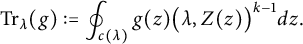 $$ \begin{align} \operatorname{Tr}_{\lambda}(g):=\oint_{c(\lambda)}g(z)\big(\lambda,Z(z)\big)^{k-1}dz. \end{align} $$
On the other hand, when $\lambda $
is split-hyperbolic, i.e., when
$\lambda $
is split-hyperbolic, i.e., when $\iota (\lambda )=1$
, the image
$\iota (\lambda )=1$
, the image $c(\lambda )$
of
$c(\lambda )$
of $c_{\lambda }$
in Y is not compact, and if g grows toward the cusps, then the integral corresponding to that from equation (4.2) does not converge. We shall regularize it only for nearly holomorphic modular forms, i.e., for
$c_{\lambda }$
in Y is not compact, and if g grows toward the cusps, then the integral corresponding to that from equation (4.2) does not converge. We shall regularize it only for nearly holomorphic modular forms, i.e., for $g\in \widetilde {M}_{2k}^{!}(\Gamma )$
. Then its Fourier expansion near the cusp associated with some
$g\in \widetilde {M}_{2k}^{!}(\Gamma )$
. Then its Fourier expansion near the cusp associated with some $\ell \in \operatorname {Iso}(V)$
is given, in the coordinates from equation (2.12), by
$\ell \in \operatorname {Iso}(V)$
is given, in the coordinates from equation (2.12), by
 $$ \begin{align} g_{\ell}(z_{\ell}):=(g\mid_{2k}\sigma_{\ell})(z_{\ell})=\sum_{l=0}^{p}\frac{g_{\ell,l}(z_{\ell})}{y_{\ell}^{l}}=\sum_{l=0}^{p}\sum_{n\in\mathbb{Z}}\frac{c_{\ell}(n,l)q_{\ell}^{n}}{y_{\ell}^{l}}= \sum_{l=0}^{p}\sum_{n\leq0}\frac{c_{\ell}(n,l)q_{\ell}^{n}}{y_{\ell}^{l}}+g_{\ell}^{0}(z_{\ell}), \end{align} $$
where p is the depth of g, $c_{\ell }(n,l)=0$
for all
$c_{\ell }(n,l)=0$
for all $0 \leq l \leq p$
when
$0 \leq l \leq p$
when $n\ll 0$
, and the latter decomposition is into the (finite) principal part and the cuspidal part
$n\ll 0$
, and the latter decomposition is into the (finite) principal part and the cuspidal part $g_{\ell }^{0}$
. Recall our extension of the incomplete Gamma function in (3.2), and the truncated modular curve
$g_{\ell }^{0}$
. Recall our extension of the incomplete Gamma function in (3.2), and the truncated modular curve $Y_{T}$
from equation (2.13) for any
$Y_{T}$
from equation (2.13) for any $T>1$
. We also set for n and
$T>1$
. We also set for n and $\kappa $
in
$\kappa $
in $\mathbb {Z}$
, positive reals c and T, split-hyperbolic
$\mathbb {Z}$
, positive reals c and T, split-hyperbolic $\lambda \in V$
, and
$\lambda \in V$
, and $g\in \widetilde {M}_{2k}^{!}(\Gamma )$
with expansion as in equation (4.3) for
$g\in \widetilde {M}_{2k}^{!}(\Gamma )$
with expansion as in equation (4.3) for $\ell =\ell _{\lambda }$
, the quantities
$\ell =\ell _{\lambda }$
, the quantities
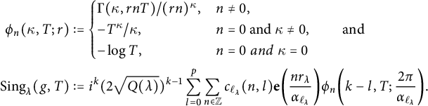 $$ \begin{align} \begin{aligned} \phi_{n}(\kappa,T;r)&:=\begin{cases} \Gamma(\kappa,rnT)/(rn)^{\kappa}, & n\neq0, \\ -T^{\kappa}/\kappa, & n=0\mathrm{\ and\ }\kappa\neq0, \\ -\log T, & n=0{\ and\ }\kappa=0 \end{cases}\qquad\mathrm{and} \\ \operatorname{Sing}_{\lambda}(g,T)&:=i^{k}(2\sqrt{Q(\lambda)})^{k-1}\sum_{l=0}^{p}\sum_{n\in\mathbb{Z}}c_{\ell_{\lambda}}(n,l)\mathbf{e}\bigg(\frac{nr_{\lambda}}{\alpha_{\ell_{\lambda}}}\bigg) \phi_{n}\bigg(k-l,T;\frac{2\pi}{\alpha_{\ell_{\lambda}}}\bigg). \end{aligned} \end{align} $$
Note that when $n=0$
,
$n=0$
, $\phi _{0}$
is independent of r, and we can then omit it from the notation. In addition, assuming that
$\phi _{0}$
is independent of r, and we can then omit it from the notation. In addition, assuming that $f\in \widetilde {M}_{2k}^{!}(\Gamma )$
expands as in equation (4.3), the weight lowering property of the operator
$f\in \widetilde {M}_{2k}^{!}(\Gamma )$
expands as in equation (4.3), the weight lowering property of the operator $L_{z}$
implies that for every
$L_{z}$
implies that for every $\nu \in \mathbb {N}$
we can write
$\nu \in \mathbb {N}$
we can write $(L_{z}^{\nu }f)_{\ell }(z_{\ell })$
as
$(L_{z}^{\nu }f)_{\ell }(z_{\ell })$
as
 $$ \begin{align} (L_{z}^{\nu}f\mid_{2k-2\nu}\sigma_{\ell})(z_{\ell})=L_{z_{\ell}}^{\nu}f_{\ell}(z_{\ell})=(-1)^{\nu}\sum_{l=\nu}^{p}\frac{l!f_{\ell,l}(z_{\ell})}{(l-\nu)!y_{\ell}^{l}}= (-1)^{\nu}\sum_{n\in\mathbb{Z}}\sum_{l=\nu}^{p}\frac{l!c_{\ell}(n,l)q_{\ell}^{n}}{(l-\nu)!y_{\ell}^{l-\nu}}. \end{align} $$
We can now define the trace to be
 $$ \begin{align} \operatorname{Tr}_{\lambda}(g):=\lim_{T\to\infty}\Bigg(\int_{c(\lambda) \cap Y_{T}}g(z)\big(\lambda,Z(z)\big)^{k-1}dz+\operatorname{Sing}_{\lambda}(g,T)+(-1)^{k}\operatorname{Sing}_{-\lambda}(g,T)\Bigg). \end{align} $$
We now prove that this is a regularization of the required trace.
Proposition 4.1 The quantity in the limit defining $\operatorname {Tr}_{\lambda }(g)$
in equation (4.6) exists and is independent of the choice of T when it is sufficiently large.
$\operatorname {Tr}_{\lambda }(g)$
in equation (4.6) exists and is independent of the choice of T when it is sufficiently large.
Proof Since $c_{\lambda }$
only intersects the cusps
$c_{\lambda }$
only intersects the cusps $\ell _{\pm \lambda }$
, there exists some
$\ell _{\pm \lambda }$
, there exists some $R>1$
such that for all
$R>1$
such that for all $T>R$
, we find that
$T>R$
, we find that $c(\lambda ) \cap Y_{T} \cong c_{\lambda }\cap \mathcal {H}_{T}$
is contained in
$c(\lambda ) \cap Y_{T} \cong c_{\lambda }\cap \mathcal {H}_{T}$
is contained in $\mathcal {H}_{R}\cup \sigma _{\ell _{\lambda }}\mathcal {F}_{T}^{\alpha _{\ell _{\lambda }}}\cup \sigma _{\ell _{-\lambda }}\mathcal {F}_{T}^{\alpha _{\ell _{-\lambda }}}$
. We thus obtain
$\mathcal {H}_{R}\cup \sigma _{\ell _{\lambda }}\mathcal {F}_{T}^{\alpha _{\ell _{\lambda }}}\cup \sigma _{\ell _{-\lambda }}\mathcal {F}_{T}^{\alpha _{\ell _{-\lambda }}}$
. We thus obtain
 $$\begin{align*}\int_{c(\lambda) \cap Y_{T}}g(z)\big(\lambda,Z(z)\big)^{k-1}dz&=\int_{c_{\lambda}\cap\mathcal{H}_{R}}\tilde{g} (z)dz+\int_{c_{\lambda}\cap\sigma_{\ell_{\lambda}}\mathcal{F}_{T}^{\alpha_{\ell_{\lambda}}}\setminus\mathcal{H}_{R}}\tilde{g}(z)dz\\ & \quad + \int_{c_{\lambda}\cap\sigma_{\ell_{-\lambda}}\mathcal{F}_{T}^{\alpha_{\ell_{-\lambda}}}\setminus\mathcal{H}_{R}}\tilde{g}(z)dz \end{align*}$$
for every $T>R$
, where we wrote
$T>R$
, where we wrote $\tilde {g}(z)$
for
$\tilde {g}(z)$
for $g(z)\big (\lambda ,Z(z)\big )^{k-1}$
. The first term is independent of T, and if we change, in the integral corresponding to
$g(z)\big (\lambda ,Z(z)\big )^{k-1}$
. The first term is independent of T, and if we change, in the integral corresponding to $\pm \lambda $
, the variable to
$\pm \lambda $
, the variable to $z_{\ell }$
for
$z_{\ell }$
for $\ell =\ell _{\pm \lambda }$
from equation (2.12), then it becomes
$\ell =\ell _{\pm \lambda }$
from equation (2.12), then it becomes
 $$\begin{align*}(\pm1)^{k}\int_{r_{\pm\lambda}+iR}^{r_{\pm\lambda}+iT}g_{\ell}(z_{\ell})\big(\sigma_{\ell}^{-1}(\pm\lambda),Z(z_{\ell})\big)^{k-1}dz_{\ell}&=(\pm i)^{k}(2\sqrt{Q(\lambda)})^{k-1}\\ & \quad \times \int_{R}^{T}g_{\ell}(r_{\pm\lambda}+iy_{\ell})y_{\ell}^{k-1}dy_{\ell} \end{align*}$$
via equation (2.17). This expression is a differentiable function of T, and equations (3.3) and (4.3) show that its derivative is minus that of $\operatorname {Sing}_{\lambda }(g,T)$
from equation (4.4). Hence, the expression from equation (4.6) is independent of T as long as
$\operatorname {Sing}_{\lambda }(g,T)$
from equation (4.4). Hence, the expression from equation (4.6) is independent of T as long as $T>R$
, and in particular
$T>R$
, and in particular $\operatorname {Tr}_{\lambda }(g)$
exists. This proves the proposition.
$\operatorname {Tr}_{\lambda }(g)$
exists. This proves the proposition.
Note that $\lim _{T\to \infty }\phi _{n}(\kappa ,T;r)=0$
for any
$\lim _{T\to \infty }\phi _{n}(\kappa ,T;r)=0$
for any $r>0$
when
$r>0$
when $n>0$
, and the integral of the part
$n>0$
, and the integral of the part $g_{\ell _{\pm \lambda }}^{0}$
from equation (4.3) converges as
$g_{\ell _{\pm \lambda }}^{0}$
from equation (4.3) converges as $T\to \infty $
. Hence, the regularization from Proposition 4.1 is essentially only of the integral of the principal part. This regularized integral can also be viewed as the special value at
$T\to \infty $
. Hence, the regularization from Proposition 4.1 is essentially only of the integral of the principal part. This regularized integral can also be viewed as the special value at $s=k$
of an appropriately regularized L-function of g, as in, e.g., [Reference Bringmann, Fricke and KentBFK].
$s=k$
of an appropriately regularized L-function of g, as in, e.g., [Reference Bringmann, Fricke and KentBFK].
Following [Reference Alfes and EhlenANS, Reference Bruinier, Funke and ImamoğluBFI], we now give an equivalent expression for the regularized theta lift $\mathcal {I}_{k,L}(\tau ,f)$
of f from equation (2.24).
$\mathcal {I}_{k,L}(\tau ,f)$
of f from equation (2.24).
Proposition 4.2 For $f\in \widetilde {M}^{!}_{2k}(\Gamma )$
with asymptotic expansion at the cusp
$f\in \widetilde {M}^{!}_{2k}(\Gamma )$
with asymptotic expansion at the cusp $\ell $
as in equation (4.3), the regularized theta lift
$\ell $
as in equation (4.3), the regularized theta lift $\mathcal {I}_{k,L}(\tau ,f)$
of f from equation (2.24) can be written as
$\mathcal {I}_{k,L}(\tau ,f)$
of f from equation (2.24) can be written as
 $$\begin{align*}\lim_{T\to\infty}\Bigg(\int_{Y_{T}}f(z)\Theta_{k,L}(\tau,z)d\mu(z)+\sum_{\ell\in\Gamma\backslash\operatorname{Iso}(V)} i^{k}\frac{\varepsilon_{\ell}}{\sqrt{N}}\Theta_{k,\ell}(\tau)\sum_{l=0}^{p}c_{\ell}(0,l) \phi_{0}(k-l,T)\Bigg), \end{align*}$$
where $\phi _{0}$
is defined in equation (
4.4
).Footnote
5
$\phi _{0}$
is defined in equation (
4.4
).Footnote
5
Proof We argue as in Proposition 5.2 of [Reference Alfes and EhlenANS], focusing on the modifications required for our statement, and leaving many details out as they are identical. For fixed T, the constant term in the integral over $Y_{T}$
is the substitution
$Y_{T}$
is the substitution $s=0$
, and near a cusp
$s=0$
, and near a cusp $\ell $
, Lemma 2.9 expresses
$\ell $
, Lemma 2.9 expresses $\Theta _{k,L}(\tau ,z)$
as a multiple of
$\Theta _{k,L}(\tau ,z)$
as a multiple of $\Theta _{k,\ell }(\tau )$
plus decreasing terms, whose integral vanishes as
$\Theta _{k,\ell }(\tau )$
plus decreasing terms, whose integral vanishes as $T\to \infty $
. Here, instead of the first equation on page 2319 of [Reference Alfes and EhlenANS], the integral of our nearly holomorphic modular form yields
$T\to \infty $
. Here, instead of the first equation on page 2319 of [Reference Alfes and EhlenANS], the integral of our nearly holomorphic modular form yields
 $$\begin{align*}\int_{1}^{\infty}\!\int_{0}^{\alpha_{\ell}}(f\mid_{2k}\sigma_{\ell}) (z_{\ell})y_{\ell}^{k-1-s}dx_{\ell}dy_{\ell}=\alpha_{\ell}\sum_{l=0}^{p}c_{\ell}(0,l)\int_{1}^{\infty} y_{\ell}^{k-s-1-l}dy_{\ell}=\alpha_{\ell}\sum_{l=0}^{p} \frac{c_{\ell}(0,l)}{k-l-s}. \end{align*}$$
The same identifications of these constant terms with our functions $\phi _{0}(k-l,T)$
yield the desired result. This proves the proposition.
$\phi _{0}(k-l,T)$
yield the desired result. This proves the proposition.
For k, $f\in \mathcal {A}_{0}^{!}(\Gamma )$
, and
$f\in \mathcal {A}_{0}^{!}(\Gamma )$
, and $g\in \mathcal {A}_{2k}^{!}(\Gamma )$
as above and an index
$g\in \mathcal {A}_{2k}^{!}(\Gamma )$
as above and an index $m\neq 0$
, we can define the combinations
$m\neq 0$
, we can define the combinations
 $$ \begin{align} \operatorname{Tr}_{m,h}^{(k)}(f):=\sum_{\lambda\in\Gamma \backslash L_{m,h}}\operatorname{Tr}_{\lambda}^{(k)}(f)\text{ for }m<0,\quad \operatorname{Tr}_{m,h}(g):=\sum_{\lambda\in\Gamma \backslash L_{m,h}}\operatorname{Tr}_{\lambda}(g)\text{ for }m>0. \end{align} $$
Note that $\Gamma \backslash L_{m,h}$
is finite when
$\Gamma \backslash L_{m,h}$
is finite when $m\neq 0$
, so that there is no question of convergence in equation (4.7). On the other hand, when
$m\neq 0$
, so that there is no question of convergence in equation (4.7). On the other hand, when $g\in \widetilde {M}^{!}_{2k}(\Gamma )$
has the usual expansion and
$g\in \widetilde {M}^{!}_{2k}(\Gamma )$
has the usual expansion and $Q(\lambda )=m=0$
, we will define the trace to be
$Q(\lambda )=m=0$
, we will define the trace to be
 $$ \begin{align} \operatorname{Tr}_{0,h}(g):=\sum_{\ell\in\Gamma\backslash\operatorname{Iso}(V)}\frac{\varepsilon_{\ell}}{\sqrt{N}}\iota_{\ell}(0,h)c_{\ell}(0,0)(\sqrt{N}\beta_{\ell})^{k}\Phi_{k}(\omega_{\ell,h}), \end{align} $$
where $\iota _{\ell }(m,h)$
,
$\iota _{\ell }(m,h)$
, $\omega _{\ell ,h}$
, and
$\omega _{\ell ,h}$
, and $\Phi _{\kappa }$
are defined in equations (2.18), (2.11), and (3.40), respectively.
$\Phi _{\kappa }$
are defined in equations (2.18), (2.11), and (3.40), respectively.
The main term of the Shintani lift from Theorem 4.3 will have the traces from equations (4.7) and (4.8) as coefficients. However, for the terms with $\iota (m)=1$
, we need to define some corrections. Recall that when
$\iota (m)=1$
, we need to define some corrections. Recall that when $m>0$
and
$m>0$
and $\iota _{\ell }(m,h)=1$
, Remark 2.7 implies that the numbers
$\iota _{\ell }(m,h)=1$
, Remark 2.7 implies that the numbers $r_{\lambda }$
for oriented
$r_{\lambda }$
for oriented $\lambda \in L_{m,h}\cap \ell ^{\perp }$
are all the same modulo
$\lambda \in L_{m,h}\cap \ell ^{\perp }$
are all the same modulo $\frac {\beta _{\ell }}{2}\sqrt {\frac {N}{m}}\mathbb {Z}$
. We can thus define, for our element
$\frac {\beta _{\ell }}{2}\sqrt {\frac {N}{m}}\mathbb {Z}$
. We can thus define, for our element $f\in \widetilde {M}^{!}_{2k}(\Gamma )$
of depth p expanded as in equation (4.3) near each cusp
$f\in \widetilde {M}^{!}_{2k}(\Gamma )$
of depth p expanded as in equation (4.3) near each cusp $\ell \in \Gamma \backslash \operatorname {Iso}(V)$
, the complementary trace
$\ell \in \Gamma \backslash \operatorname {Iso}(V)$
, the complementary trace
 $$ \begin{align} \begin{aligned} &\operatorname{Tr}^{\mathrm{c}}_{m,h}(f,v):=-(-2i\sqrt{m})^{k}\cdot\sqrt{2\pi}\sum_{\ell\in\Gamma\backslash\operatorname{Iso}(V)} \big(\iota_{\ell}(m,h)+(-1)^{k}\iota_{\ell}(m,-h)\big)\frac{\varepsilon_{\ell}}{\sqrt{N}} \\ &\times\sum_{\substack{0>n\in\mathbb{Z} \\ n\equiv0\bmod 2\varepsilon_{\ell}\sqrt{m/N}}}\mathbf{e}\bigg(\frac{nr_{\lambda}}{\alpha_{\ell}}\bigg)\sum_{l=k}^{p}\bigg(\frac{2\pi n}{\alpha_{\ell}}\bigg)^{l-k}\frac{l!c_{\ell}(n,l)}{(l-k)!}\cdot\frac{J_{l}\big(2\sqrt{2\pi mv}\big)}{\big(2\sqrt{2\pi mv}\big)^{l}}, \end{aligned} \end{align} $$
with $J_{l}(\eta )$
from equation (3.31). Note that the sum over n in equation (4.9) is finite, and is empty for all but finitely many values of m.
$J_{l}(\eta )$
from equation (3.31). Note that the sum over n in equation (4.9) is finite, and is empty for all but finitely many values of m.
We also define the complementary trace from constants
 $$ \begin{align} \begin{aligned} &\operatorname{Tr}^{\mathrm{cc}}_{m,h}(f,v):=-(-2i\sqrt{m})^{k}\sum_{\ell\in\Gamma\backslash\operatorname{Iso}(V)} \big(\iota_{\ell}(m,h)+(-1)^{k}\iota_{\ell}(m,-h)\big)\frac{\varepsilon_{\ell}}{\sqrt{N}} \\ &\times k!c_{\ell}(0,k)\frac{I_{k}\big(2\sqrt{2\pi mv}\big)-\tilde{\Omega}_{k}\big(2\sqrt{2\pi mv}\big)}{\big(2\sqrt{2\pi mv}\big)^{k}}, \end{aligned} \end{align} $$
where $I_{k}$
and
$I_{k}$
and $\tilde {\Omega }_{k}$
are defined in equation (3.26) and Remark 3.13, respectively. The name represents the fact that only the constant terms
$\tilde {\Omega }_{k}$
are defined in equation (3.26) and Remark 3.13, respectively. The name represents the fact that only the constant terms $c_{\ell }(0,k)$
contribute to it.
$c_{\ell }(0,k)$
contribute to it.
When $m=0$
, there is only a complementary trace from constants, which is defined as
$m=0$
, there is only a complementary trace from constants, which is defined as
 $$ \begin{align} \begin{aligned} &\operatorname{Tr}^{\mathrm{cc}}_{0,h}(f,v):=\delta_{k,0}\delta_{h,0}\sqrt{v} \int_{Y}^{{\mathrm{reg}}}f(z)d\mu(z)+\sum_{\ell\in\Gamma\backslash\operatorname{Iso}(V)}\iota_{\ell}(0,h) \frac{\varepsilon_{\ell}}{\sqrt{N}}\times \\ &\Bigg(\kern-2pt -k!c_{\ell}(0,k)P_{k}(0)\frac{\log\big(\sqrt{2\pi Nv}\beta_{\ell}\big)+C_{k}}{(2\pi v)^{k/2}}+\sum_{l=0}^{p}l!c_{\ell}(0,l)Q_{l}(0)\frac{(\sqrt{N}\beta_{\ell})^{k-l}\Xi_{k-l}(\omega_{\ell,h})}{(2\pi v)^{l/2}}\kern-2pt\Bigg), \end{aligned} \end{align} $$
where $C_{k}$
and
$C_{k}$
and $\Xi _{\kappa }$
are defined in equations (3.43) and (3.41) respectively, and for
$\Xi _{\kappa }$
are defined in equations (3.43) and (3.41) respectively, and for $f\in \widetilde {M}^{!}_{2k}(\Gamma )$
, the regularized integral
$f\in \widetilde {M}^{!}_{2k}(\Gamma )$
, the regularized integral $\int _{Y}^{{\mathrm {reg}}}f(z)d\mu (z)$
is the (convergent) limit
$\int _{Y}^{{\mathrm {reg}}}f(z)d\mu (z)$
is the (convergent) limit $\lim _{T\to \infty }\int _{Y_{T}}f(z)d\mu (z)$
.
$\lim _{T\to \infty }\int _{Y_{T}}f(z)d\mu (z)$
.
4.2 Main theorem and proof
We can now state and prove our main theorem. Given $k\in \mathbb {N}$
and an element
$k\in \mathbb {N}$
and an element $f\in \widetilde {M}_{2k}^{!}(\Gamma )$
, we gather the traces from equations (4.7) and (4.8) and define
$f\in \widetilde {M}_{2k}^{!}(\Gamma )$
, we gather the traces from equations (4.7) and (4.8) and define
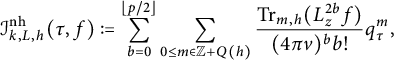 $$ \begin{align} \mathcal{I}_{k,L,h}^{\mathrm{nh}}(\tau,f):=\sum_{b=0}^{\lfloor p/2 \rfloor}\sum_{0 \leq m\in\mathbb{Z}+Q(h)}\frac{\operatorname{Tr}_{m,h}(L_{z}^{2b}f)}{(4\pi v)^{b}b!}q_{\tau}^{m}, \end{align} $$
which is a nearly holomorphic function of depth $\big \lfloor \frac {p}{2}\big \rfloor $
on
$\big \lfloor \frac {p}{2}\big \rfloor $
on $\mathcal {H}$
that is bounded at
$\mathcal {H}$
that is bounded at $\infty $
. Using the negative index case of equation (4.7), we also define
$\infty $
. Using the negative index case of equation (4.7), we also define
 $$ \begin{align} \mathcal{I}_{k,L,h}^{\mathrm{neg}}(\tau,f):=\sum_{0>m\in\mathbb{Z}+Q(h)}\sum_{l=k}^{p}\frac{4^{k}\sqrt{\pi}|m|^{\frac{k-1}{2}}h_{l}\big(2\sqrt{2\pi|m|v}\big)}{\sqrt{2}\big(4\sqrt{2\pi|m|v}\big)^{l}(l-k)!} \operatorname{Tr}_{m,h}^{(k)}(R_{2k-2l}^{l-k}L_{z}^{l}f)q_{\tau}^{m}, \end{align} $$
which resembles the non-holomorphic part of a harmonic weak Maass form with cuspidal $\xi $
-image (see also the proof of Proposition 4.5). We also gather the traces from equations 4.9–4.11, and set
$\xi $
-image (see also the proof of Proposition 4.5). We also gather the traces from equations 4.9–4.11, and set
 $$ \begin{align} \mathcal{I}_{k,L,h}^{\mathrm{c}}(\tau,f):=\sum_{\substack{0<m\in\mathbb{Z}+Q(h) \\ \iota(m)=1}}\!\operatorname{Tr}^{\mathrm{c}}_{m,h}(f,v)q_{\tau}^{m}\quad\mathrm{and}\quad\mathcal{I}_{k,L,h}^{\mathrm{cc}}(\tau,f):=\sum_{\substack{0 \leq m\in\mathbb{Z}+Q(h) \\ \iota(m)=1}}\!\operatorname{Tr}^{\mathrm{cc}}_{m,h}(f,v)q_{\tau}^{m}, \end{align} $$
where the former is a finite sum of increasing terms, and the second one is infinite but converges.
The main result, which evaluates the regularized Shintani lift of f, now reads as follows.
Theorem 4.3 Write the vector-valued Shintani lift $\mathcal {I}_{k,L}(\tau ,f)$
of
$\mathcal {I}_{k,L}(\tau ,f)$
of $f\in \widetilde {M}_{2k}^{!}(\Gamma )$
, which is defined in equation (2.24) and lies in
$f\in \widetilde {M}_{2k}^{!}(\Gamma )$
, which is defined in equation (2.24) and lies in $\mathcal {A}_{k+\frac {1}{2}}\big (\operatorname {Mp}_{2}(\mathbb {Z}),\rho _{L}\big )$
, as
$\mathcal {A}_{k+\frac {1}{2}}\big (\operatorname {Mp}_{2}(\mathbb {Z}),\rho _{L}\big )$
, as $\sum _{h \in D_{L}}\mathcal {I}_{k,L,h}(\tau ,f)\mathfrak {e}_{h}$
. Then the scalar-valued coefficient associated with
$\sum _{h \in D_{L}}\mathcal {I}_{k,L,h}(\tau ,f)\mathfrak {e}_{h}$
. Then the scalar-valued coefficient associated with $h \in D_{L}$
is given by
$h \in D_{L}$
is given by
 $$\begin{align*}\mathcal{I}_{k,L,h}(\tau,f)=\mathcal{I}_{k,L,h}^{\mathrm{nh}}(\tau,f)+\mathcal{I}_{k,L,h}^{\mathrm{neg}}(\tau,f)+\mathcal{I}_{k,L,h}^{\mathrm{c}}(\tau,f)+\mathcal{I}_{k,L,h}^{\mathrm{cc}}(\tau,f),\end{align*}$$
Proof We apply Proposition 4.2, and expand $\Theta _{k,L}(\tau ,z)$
and
$\Theta _{k,L}(\tau ,z)$
and $\Theta _{k,\ell }(\tau )$
using equations (3.21) and (2.23) respectively, which gives
$\Theta _{k,\ell }(\tau )$
using equations (3.21) and (2.23) respectively, which gives
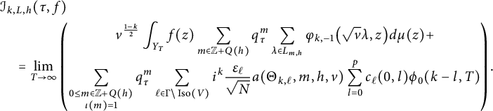 $$ \begin{align} \\[-3pc] &\mathcal{I}_{k,L,h}(\tau,f)\nonumber \\ &\quad =\lim_{T\to\infty}\left(\!\!\!\begin{array}{c}\displaystyle v^{\frac{1-k}{2}}\int_{Y_{T}}f(z)\sum_{m\in\mathbb{Z}+Q(h)}q_{\tau}^{m}\sum_{\lambda \in L_{m,h}}\varphi_{k,-1}\big(\sqrt{v}\lambda,z\big)d\mu(z)+ \\ \displaystyle\sum_{\substack{0 \leq m\in\mathbb{Z}+Q(h) \\ \iota(m)=1}}q_{\tau}^{m}\sum_{\ell\in\Gamma\backslash\operatorname{Iso}(V)}i^{k}\frac{\varepsilon_{\ell}}{\sqrt{N}}a(\Theta_{k,\ell},m,h,v)\sum_{l=0}^{p}c_{\ell}(0,l)\phi_{0}(k-l,T)\end{array}\!\!\!\!\right).\nonumber \end{align} $$
We may interchange the order of integration and summation as both are absolutely convergent for fixed T. Propositions 4.10–4.13 now evaluate the coefficient of $q_{\tau }^{m}$
to be the one implied by the asserted sum. This proves the theorem.
$q_{\tau }^{m}$
to be the one implied by the asserted sum. This proves the theorem.
A much simpler but interesting special case is the one where the depth $p<k$
.
$p<k$
.
Corollary 4.4 Assume that $f\in \widetilde {M}_{2k}^{!,\leq p}(\Gamma )$
, and that
$f\in \widetilde {M}_{2k}^{!,\leq p}(\Gamma )$
, and that $p<k$
. Then
$p<k$
. Then
 $$\begin{align*}\mathcal{I}_{k,L}(\tau,f)=\sum_{h \in D_{L}}\mathcal{I}^{\mathrm{nh}}_{k,L,h}(\tau,f)\mathfrak{e}_{h}\in\widetilde{M}_{k+\frac{1}{2}}^{\leq\lfloor p/2 \rfloor}\big(\operatorname{Mp}_{2}(\mathbb{Z}),\rho_{L}\big).\end{align*}$$
For $p=0$
, we recover the part of Theorem 6.1 of [Reference Alfes and EhlenANS] with weakly holomorphic input.
$p=0$
, we recover the part of Theorem 6.1 of [Reference Alfes and EhlenANS] with weakly holomorphic input.
Proof If $p<k$
, then
$p<k$
, then $\mathcal {I}^{\mathrm {neg}}_{k,L,h}$
and
$\mathcal {I}^{\mathrm {neg}}_{k,L,h}$
and $\mathcal {I}^{\mathrm {c}}_{k,L,h}$
vanish identically (because both involve sums over
$\mathcal {I}^{\mathrm {c}}_{k,L,h}$
vanish identically (because both involve sums over $k \leq l \leq p$
), and equations (4.10) and (4.11) imply that
$k \leq l \leq p$
), and equations (4.10) and (4.11) imply that $\mathcal {I}^{\mathrm {cc}}_{k,L,h}$
consists only of the constant term
$\mathcal {I}^{\mathrm {cc}}_{k,L,h}$
consists only of the constant term
 $$\begin{align*}\operatorname{Tr}^{\mathrm{cc}}_{0,h}(f,v)= \sum_{\ell\in\Gamma\backslash\operatorname{Iso}(V)}\iota_{\ell}(0,h)\frac{\varepsilon_{\ell}}{\sqrt{N}}\sum_{l=0}^{k-1}l!c_{\ell}(0,l)Q_{l}(0) \frac{(\sqrt{N}\beta_{\ell})^{k-l}\Xi_{k-l}(\omega_{\ell,h})}{(2\pi v)^{l/2}} \end{align*}$$
(because $c_{\ell }(0,k)=0$
when
$c_{\ell }(0,k)=0$
when $p<k$
). Since
$p<k$
). Since $k-l>0$
, the only term
$k-l>0$
, the only term $\Xi _{k-l}(\omega _{\ell ,h})$
from equation (3.41) that may not vanish is when
$\Xi _{k-l}(\omega _{\ell ,h})$
from equation (3.41) that may not vanish is when $l=k-1$
and
$l=k-1$
and $\omega _{\ell ,h}=0$
, where it equals the constant
$\omega _{\ell ,h}=0$
, where it equals the constant $-\frac {1}{\sqrt {2\pi }}$
. However, equation (2.11) shows that the latter equality only holds when
$-\frac {1}{\sqrt {2\pi }}$
. However, equation (2.11) shows that the latter equality only holds when $h=0$
, and thus equation (2.18) yields
$h=0$
, and thus equation (2.18) yields $\iota _{\ell }(0,h)=1$
for all
$\iota _{\ell }(0,h)=1$
for all $\ell $
, and the terms involving
$\ell $
, and the terms involving $\varepsilon _{\ell }$
,
$\varepsilon _{\ell }$
, $\beta _{\ell }$
, and
$\beta _{\ell }$
, and $\sqrt {N}$
reduce to
$\sqrt {N}$
reduce to $\alpha _{\ell }$
when
$\alpha _{\ell }$
when $l=k-1$
by equation (2.10). This reduces our expression for
$l=k-1$
by equation (2.10). This reduces our expression for $\mathcal {I}^{\mathrm {cc}}_{k,L,h}$
to
$\mathcal {I}^{\mathrm {cc}}_{k,L,h}$
to $-\frac {Q_{k-1}(0)}{(2\pi )^{k/2}v^{(k-1)/2}}$
times
$-\frac {Q_{k-1}(0)}{(2\pi )^{k/2}v^{(k-1)/2}}$
times $\sum _{\ell }\alpha _{\ell }c_{\ell }(0,k-1)$
. However, the
$\sum _{\ell }\alpha _{\ell }c_{\ell }(0,k-1)$
. However, the $c_{\ell }(0,k-1)$
’s are, up to constant multiple that is independent of
$c_{\ell }(0,k-1)$
’s are, up to constant multiple that is independent of $\ell $
, the constant terms of the weakly holomorphic modular form
$\ell $
, the constant terms of the weakly holomorphic modular form $L_{z}^{k-1}f \in M_{2}^{!}(\Gamma )$
, and by equation (2.12), multiplying each by
$L_{z}^{k-1}f \in M_{2}^{!}(\Gamma )$
, and by equation (2.12), multiplying each by $\alpha _{\ell }$
yields the residue of the corresponding meromorphic differential
$\alpha _{\ell }$
yields the residue of the corresponding meromorphic differential $L_{z}^{k-1}fdz$
at the cusp
$L_{z}^{k-1}fdz$
at the cusp $\ell $
(again, up to a constant multiple that is independent of
$\ell $
(again, up to a constant multiple that is independent of $\ell $
). Thus,
$\ell $
). Thus, $\mathcal {I}^{\mathrm {cc}}_{k,L,h}$
is a multiple of the sum of residues of a meromorphic differential on the compact curve associated with
$\mathcal {I}^{\mathrm {cc}}_{k,L,h}$
is a multiple of the sum of residues of a meromorphic differential on the compact curve associated with $\Gamma $
at all of its poles, which therefore vanishes (this also explains Remark 1.4). This proves the corollary.
$\Gamma $
at all of its poles, which therefore vanishes (this also explains Remark 1.4). This proves the corollary.
When $p \geq k$
, Corollary 4.4 no longer holds, but one can obtain a nearly holomorphic modular form after applying an appropriate weight-changing operator.
$p \geq k$
, Corollary 4.4 no longer holds, but one can obtain a nearly holomorphic modular form after applying an appropriate weight-changing operator.
Proposition 4.5 For any $f\in \widetilde {M}_{2k}^{!,\leq p}(\Gamma )$
for which the constant terms
$f\in \widetilde {M}_{2k}^{!,\leq p}(\Gamma )$
for which the constant terms $c_{\ell }(0,k)$
vanish for every
$c_{\ell }(0,k)$
vanish for every $\ell $
, we have
$\ell $
, we have
 $$\begin{align*}\xi_{k-2\lfloor p/2 \rfloor+\frac{1}{2}}L_{\tau}^{\lfloor p/2 \rfloor}\mathcal{I}_{k,L}(\tau,f)\in\widetilde{M}_{2\lfloor p/2 \rfloor-k+\frac{3}{2}}^{\leq p-k}\big(\operatorname{Mp}_{2}(\mathbb{Z}),\overline{\rho}_{L}\big). \end{align*}$$
Note that, for $p<k$
, the depth is negative, so that the space
$p<k$
, the depth is negative, so that the space $\widetilde {M}_{2\lfloor p/2 \rfloor -k+\frac {3}{2}}^{\leq p-k}(\overline {\rho }_{L})$
is trivial, and indeed the modular forms that are annihilated by the operator in question are those lying in
$\widetilde {M}_{2\lfloor p/2 \rfloor -k+\frac {3}{2}}^{\leq p-k}(\overline {\rho }_{L})$
is trivial, and indeed the modular forms that are annihilated by the operator in question are those lying in $\widetilde {M}_{k+\frac {1}{2}}^{\leq \lfloor p/2 \rfloor }\big (\operatorname {Mp}_{2}(\mathbb {Z}),\rho _{L}\big )$
.
$\widetilde {M}_{k+\frac {1}{2}}^{\leq \lfloor p/2 \rfloor }\big (\operatorname {Mp}_{2}(\mathbb {Z}),\rho _{L}\big )$
.
Proof The fact that $\xi _{k-2\lfloor p/2 \rfloor +\frac {1}{2}}L_{\tau }^{\lfloor p/2 \rfloor }\mathcal {I}_{k,L}(\tau ,f)$
lies in
$\xi _{k-2\lfloor p/2 \rfloor +\frac {1}{2}}L_{\tau }^{\lfloor p/2 \rfloor }\mathcal {I}_{k,L}(\tau ,f)$
lies in $\mathcal {A}_{2\lfloor p/2 \rfloor -k+\frac {3}{2}}\big (\operatorname {Mp}_{2}(\mathbb {Z}),\overline {\rho }_{L}\big )$
follows from the weight changing properties of
$\mathcal {A}_{2\lfloor p/2 \rfloor -k+\frac {3}{2}}\big (\operatorname {Mp}_{2}(\mathbb {Z}),\overline {\rho }_{L}\big )$
follows from the weight changing properties of $L_{\tau }$
and
$L_{\tau }$
and $\xi _{k-2\lfloor p/2 \rfloor +\frac {1}{2}}$
, including the conjugation of the representation in equation (3.41). For investigating its analytic properties, we need to evaluate the operation of
$\xi _{k-2\lfloor p/2 \rfloor +\frac {1}{2}}$
, including the conjugation of the representation in equation (3.41). For investigating its analytic properties, we need to evaluate the operation of $L_{\tau }$
on each of the summands in Theorem 4.3.
$L_{\tau }$
on each of the summands in Theorem 4.3.
The first summand, from equation (4.12), is nearly holomorphic of depth $\big \lfloor \frac {p}{2}\big \rfloor $
. Every application of
$\big \lfloor \frac {p}{2}\big \rfloor $
. Every application of $L_{\tau }$
reduces the depth by 1, and then the application of the
$L_{\tau }$
reduces the depth by 1, and then the application of the $\xi $
-operator, which is again
$\xi $
-operator, which is again $L_{\tau }$
composed with a modified complex conjugation, annihilates the weakly holomorphic expression
$L_{\tau }$
composed with a modified complex conjugation, annihilates the weakly holomorphic expression $L_{\tau }^{\lfloor p/2 \rfloor }\mathcal {I}_{k,L,h}^{\mathrm {nh}}(\tau ,f)$
. Now, the terms from equation (4.13), as well as those from equation (4.14) defined in equation (4.9), involve the expressions
$L_{\tau }^{\lfloor p/2 \rfloor }\mathcal {I}_{k,L,h}^{\mathrm {nh}}(\tau ,f)$
. Now, the terms from equation (4.13), as well as those from equation (4.14) defined in equation (4.9), involve the expressions $\frac {h_{l}(\eta )}{\eta ^{l}}$
and
$\frac {h_{l}(\eta )}{\eta ^{l}}$
and $\frac {J_{l}(\eta )}{\eta ^{l}}$
respectively, for
$\frac {J_{l}(\eta )}{\eta ^{l}}$
respectively, for $\eta =2\sqrt {2\pi |m|v}$
and
$\eta =2\sqrt {2\pi |m|v}$
and $k \leq l \leq p$
, times constants times
$k \leq l \leq p$
, times constants times $q_{\tau }^{m}$
. As applying
$q_{\tau }^{m}$
. As applying $L_{\tau }=-2iv^{2}\partial _{\overline {\tau }}$
to a function of
$L_{\tau }=-2iv^{2}\partial _{\overline {\tau }}$
to a function of $\eta $
is the same as
$\eta $
is the same as $\frac {\eta ^{3}}{16\pi |m|}\frac {d}{d\eta }$
, Lemma 3.16 and equation (3.32) imply that this effect amounts, up to scalar multiples, to subtracting 2 from the index l. After doing so
$\frac {\eta ^{3}}{16\pi |m|}\frac {d}{d\eta }$
, Lemma 3.16 and equation (3.32) imply that this effect amounts, up to scalar multiples, to subtracting 2 from the index l. After doing so $\big \lfloor \frac {p}{2}\big \rfloor +1$
times (including the action of the
$\big \lfloor \frac {p}{2}\big \rfloor +1$
times (including the action of the $\xi $
-operator), we remain only with indices
$\xi $
-operator), we remain only with indices $k-2\big \lfloor \frac {p}{2}\big \rfloor -2 \leq l \leq p-2\big \lfloor \frac {p}{2}\big \rfloor -2$
, that are thus negative.
$k-2\big \lfloor \frac {p}{2}\big \rfloor -2 \leq l \leq p-2\big \lfloor \frac {p}{2}\big \rfloor -2$
, that are thus negative.
However, equations (3.17) and (3.31), the vanishing of $P_{\nu }$
and
$P_{\nu }$
and $\widetilde {P}_{\nu }$
via Remark 3.8 and equation (3.30), and the parity of
$\widetilde {P}_{\nu }$
via Remark 3.8 and equation (3.30), and the parity of $Q_{\nu }$
and
$Q_{\nu }$
and $\widetilde {Q}_{\nu }$
imply that for negative l, such expressions are odd polynomials in
$\widetilde {Q}_{\nu }$
imply that for negative l, such expressions are odd polynomials in $\eta $
, of degree at most
$\eta $
, of degree at most $4\big \lfloor \frac {p}{2}\big \rfloor +3-2k$
multiplied by
$4\big \lfloor \frac {p}{2}\big \rfloor +3-2k$
multiplied by $e^{\pm \eta ^{2}/2}$
respectively. Recalling that for the effect of
$e^{\pm \eta ^{2}/2}$
respectively. Recalling that for the effect of $\xi _{k-2\lfloor p/2 \rfloor +\frac {1}{2}}$
we must conjugate and multiply by v to the negative half-integral power
$\xi _{k-2\lfloor p/2 \rfloor +\frac {1}{2}}$
we must conjugate and multiply by v to the negative half-integral power $k-2\big \lfloor \frac {p}{2}\big \rfloor -\frac {3}{2}$
, and substituting the value
$k-2\big \lfloor \frac {p}{2}\big \rfloor -\frac {3}{2}$
, and substituting the value $2\sqrt {2\pi |m|v}$
of
$2\sqrt {2\pi |m|v}$
of $\eta $
, we indeed obtain a decaying nearly holomorphic expression from the image of
$\eta $
, we indeed obtain a decaying nearly holomorphic expression from the image of $\mathcal {I}_{k,L,h}^{\mathrm {neg}}(\tau ,f)$
for each
$\mathcal {I}_{k,L,h}^{\mathrm {neg}}(\tau ,f)$
for each $h \in D_{L}$
, and a finite increasing nearly holomorphic expression from the image of
$h \in D_{L}$
, and a finite increasing nearly holomorphic expression from the image of $\mathcal {I}_{k,L,h}^{\mathrm {c}}(\tau ,f)$
for every h. For the depth bound, we need the lowest power of
$\mathcal {I}_{k,L,h}^{\mathrm {c}}(\tau ,f)$
for every h. For the depth bound, we need the lowest power of $\eta $
in the expressions
$\eta $
in the expressions $\eta ^{|l|}Q_{l}(\eta )$
or
$\eta ^{|l|}Q_{l}(\eta )$
or $\eta ^{|l|}\widetilde {Q}_{l}(\eta )$
for negative l in our range, which arises from the value
$\eta ^{|l|}\widetilde {Q}_{l}(\eta )$
for negative l in our range, which arises from the value $p-2\big \lfloor \frac {p}{2}\big \rfloor -2$
of l that is minimal in absolute value, divided by
$p-2\big \lfloor \frac {p}{2}\big \rfloor -2$
of l that is minimal in absolute value, divided by $\eta ^{4\lfloor p/2 \rfloor +3-2k}$
. For odd p, this is
$\eta ^{4\lfloor p/2 \rfloor +3-2k}$
. For odd p, this is $l=-1$
with
$l=-1$
with $\eta $
multiplied by a constant term, yielding a denominator of
$\eta $
multiplied by a constant term, yielding a denominator of $v^{2\lfloor p/2 \rfloor +1-k}=v^{p-k}$
, and if p is even then
$v^{2\lfloor p/2 \rfloor +1-k}=v^{p-k}$
, and if p is even then $l=-2$
is multiplied by a linear polynomial in
$l=-2$
is multiplied by a linear polynomial in $\eta $
, and the denominator is
$\eta $
, and the denominator is $v^{2\lfloor p/2 \rfloor -k}=v^{p-k}$
as well.
$v^{2\lfloor p/2 \rfloor -k}=v^{p-k}$
as well.
It remains to consider the constant terms in equation (4.14), defined in equation (4.11). The first term, appearing only when $k=0$
, is a multiple of
$k=0$
, is a multiple of $\sqrt {v}$
, which after
$\sqrt {v}$
, which after $\big \lfloor \frac {p}{2}\big \rfloor +1$
operations of
$\big \lfloor \frac {p}{2}\big \rfloor +1$
operations of $L_{\tau }$
becomes a multiple of
$L_{\tau }$
becomes a multiple of $v^{\lfloor p/2 \rfloor +3/2}$
, and after conjugating and multiplying by
$v^{\lfloor p/2 \rfloor +3/2}$
, and after conjugating and multiplying by $v^{-2\lfloor p/2 \rfloor -\frac {3}{2}}$
(with
$v^{-2\lfloor p/2 \rfloor -\frac {3}{2}}$
(with $k=0$
) yields
$k=0$
) yields $v^{-\lfloor p/2 \rfloor }$
, indeed nearly holomorphic with the required degree bound. Similarly,
$v^{-\lfloor p/2 \rfloor }$
, indeed nearly holomorphic with the required degree bound. Similarly, $\big \lfloor \frac {p}{2}\big \rfloor +1$
actions of
$\big \lfloor \frac {p}{2}\big \rfloor +1$
actions of $L_{\tau }$
and multiplication by
$L_{\tau }$
and multiplication by $v^{k-2\lfloor p/2 \rfloor -\frac {3}{2}}$
take the lth term in the last in equation (4.11) to a multiple of
$v^{k-2\lfloor p/2 \rfloor -\frac {3}{2}}$
take the lth term in the last in equation (4.11) to a multiple of $v^{k-\lfloor p/2 \rfloor -\frac {l+1}{2}}$
. Since the multiplier
$v^{k-\lfloor p/2 \rfloor -\frac {l+1}{2}}$
. Since the multiplier $Q_{l}(0)$
restricts l to be odd, and with
$Q_{l}(0)$
restricts l to be odd, and with $l \leq p$
the maximal value of
$l \leq p$
the maximal value of $\frac {l+1}{2}$
is
$\frac {l+1}{2}$
is $\big \lceil \frac {p}{2}\big \rceil $
, the result here is nearly holomorphic of degree at most
$\big \lceil \frac {p}{2}\big \rceil $
, the result here is nearly holomorphic of degree at most $p-k$
. As this covers all the expressions that are not multiples of the coefficients
$p-k$
. As this covers all the expressions that are not multiples of the coefficients $c_{\ell }(0,k)$
, this proves the proposition.
$c_{\ell }(0,k)$
, this proves the proposition.
Remark 4.6 A natural question to ask, in view of Proposition 4.5, is what can be said about the $\xi _{k-2\lfloor p/2 \rfloor +\frac {1}{2}}L_{\tau }^{\lfloor p/2 \rfloor }\mathcal {I}_{k,L}(\tau ,f)$
in case the coefficients
$\xi _{k-2\lfloor p/2 \rfloor +\frac {1}{2}}L_{\tau }^{\lfloor p/2 \rfloor }\mathcal {I}_{k,L}(\tau ,f)$
in case the coefficients $c_{\ell }(0,k)$
do not vanish. Following the proof of that proposition, the terms involving
$c_{\ell }(0,k)$
do not vanish. Following the proof of that proposition, the terms involving $\frac {I_{k}(\eta )}{\eta ^{k}}$
from equation (4.10) inside equation (4.14) behave like those with
$\frac {I_{k}(\eta )}{\eta ^{k}}$
from equation (4.10) inside equation (4.14) behave like those with $\frac {h_{l}(\eta )}{\eta ^{l}}$
or
$\frac {h_{l}(\eta )}{\eta ^{l}}$
or $\frac {J_{l}(\eta )}{\eta ^{l}}$
(see Lemma 3.21 and equation (3.29)), and as the polynomial
$\frac {J_{l}(\eta )}{\eta ^{l}}$
(see Lemma 3.21 and equation (3.29)), and as the polynomial $\tilde {\Omega }_{k}$
from Remark 3.13 has degree
$\tilde {\Omega }_{k}$
from Remark 3.13 has degree $k-2$
and parity
$k-2$
and parity $(-1)^{k}$
, the corresponding expression from equation (4.10) is nearly holomorphic of degree at most
$(-1)^{k}$
, the corresponding expression from equation (4.10) is nearly holomorphic of degree at most $\big \lfloor \frac {p}{2}\big \rfloor $
and is thus annihilated by
$\big \lfloor \frac {p}{2}\big \rfloor $
and is thus annihilated by $L_{\tau }^{\lfloor p/2 \rfloor }$
. Now, we can express
$L_{\tau }^{\lfloor p/2 \rfloor }$
. Now, we can express $I_{\nu }$
for
$I_{\nu }$
for $\nu :=k-2\big \lfloor \frac {p}{2}\big \rfloor -2<0$
via equation (3.29), where using equation (3.8) the multiplier of
$\nu :=k-2\big \lfloor \frac {p}{2}\big \rfloor -2<0$
via equation (3.29), where using equation (3.8) the multiplier of $I_{-1}$
becomes a multiple of
$I_{-1}$
becomes a multiple of $P_{-1-\nu }$
. As one can verify by induction that the polynomial
$P_{-1-\nu }$
. As one can verify by induction that the polynomial $\hat {\Omega }_{\nu }$
from equation (3.29) equals minus the same multiple of
$\hat {\Omega }_{\nu }$
from equation (3.29) equals minus the same multiple of $Q_{-1-\nu }$
for
$Q_{-1-\nu }$
for $\nu <0$
, this determines
$\nu <0$
, this determines $I_{\nu }(\eta )$
as a multiple of
$I_{\nu }(\eta )$
as a multiple of $e^{\eta ^{2}/2}h_{-1-\nu }(\eta )$
, and with the powers of m and v, this evaluates the image of the expression from equation (4.10) under
$e^{\eta ^{2}/2}h_{-1-\nu }(\eta )$
, and with the powers of m and v, this evaluates the image of the expression from equation (4.10) under $\xi _{k-2\lfloor p/2 \rfloor +\frac {1}{2}}L_{\tau }^{\lfloor p/2 \rfloor }$
as a multiple of
$\xi _{k-2\lfloor p/2 \rfloor +\frac {1}{2}}L_{\tau }^{\lfloor p/2 \rfloor }$
as a multiple of $\frac {h_{|\nu |-1}(\eta )}{\eta ^{|\nu |-1}}q_{\tau }^{-m}$
with our
$\frac {h_{|\nu |-1}(\eta )}{\eta ^{|\nu |-1}}q_{\tau }^{-m}$
with our $\eta $
. The term with the scalar and the logarithm in the constant term from equation (4.11), which shows up only for even k because of the multiplier
$\eta $
. The term with the scalar and the logarithm in the constant term from equation (4.11), which shows up only for even k because of the multiplier $P_{k}(0)$
, becomes, after this operator, a constant divided by
$P_{k}(0)$
, becomes, after this operator, a constant divided by $v^{\frac {|\nu |-1}{2}}$
. Recall that the nearly holomorphic part from Proposition 4.5 is annihilated after applying
$v^{\frac {|\nu |-1}{2}}$
. Recall that the nearly holomorphic part from Proposition 4.5 is annihilated after applying $\xi _{k-\lceil p/2 \rceil +\frac {3}{2}}L_{\tau }^{k-p}$
, so one can apply this operator to the remaining expression. Using similar considerations once again, and verifying that all the multipliers match (including the constant terms) shows, via equation (2.23), that the resulting expression is a constant multiple of the sum
$\xi _{k-\lceil p/2 \rceil +\frac {3}{2}}L_{\tau }^{k-p}$
, so one can apply this operator to the remaining expression. Using similar considerations once again, and verifying that all the multipliers match (including the constant terms) shows, via equation (2.23), that the resulting expression is a constant multiple of the sum $\sum _{\ell \in \Gamma \backslash \operatorname {Iso}(V)}c_{\ell }(0,k)\Theta _{2\lceil p/2 \rceil -k,\ell }(\tau )$
. In total, for
$\sum _{\ell \in \Gamma \backslash \operatorname {Iso}(V)}c_{\ell }(0,k)\Theta _{2\lceil p/2 \rceil -k,\ell }(\tau )$
. In total, for $p<k$
, the Shintani lift is annihilated by one application of
$p<k$
, the Shintani lift is annihilated by one application of $\xi _{*}L_{\tau }^{*}$
(by Corollary 4.4), when
$\xi _{*}L_{\tau }^{*}$
(by Corollary 4.4), when $p \geq k$
and
$p \geq k$
and $c_{\ell }(0,k)=0$
for all
$c_{\ell }(0,k)=0$
for all $\ell $
, it is killed after two applications of such operators, resembling harmonicity (this is Proposition 4.5), and with the extra term, a third application is required for sending the lift to 0, which is a type of a sesqui-harmonic property (because the theta function from equation (2.23) is nearly holomorphic itself).
$\ell $
, it is killed after two applications of such operators, resembling harmonicity (this is Proposition 4.5), and with the extra term, a third application is required for sending the lift to 0, which is a type of a sesqui-harmonic property (because the theta function from equation (2.23) is nearly holomorphic itself).
We can now deduce the theorems mentioned in the Introduction.
Proof of Theorem 1.1
We apply Theorem 4.3 to the scaled lattice $L_{\Delta }:=\Delta L$
for L from equation (2.8), with
$L_{\Delta }:=\Delta L$
for L from equation (2.8), with $Q=-\frac {\det }{|\Delta |}$
. Then
$Q=-\frac {\det }{|\Delta |}$
. Then $L_{\Delta }^{*}=L^{*}$
and it is well known (see [Reference Gross, Kohnen and ZagierGKZ] or [Reference Alfes-Neumann and SchwagenscheidtAE]) that if
$L_{\Delta }^{*}=L^{*}$
and it is well known (see [Reference Gross, Kohnen and ZagierGKZ] or [Reference Alfes-Neumann and SchwagenscheidtAE]) that if $g\in \mathcal {A}_{\frac {3}{2}}^{!}\big (\operatorname {Mp}_{2}(\mathbb {Z}),\rho _{L_{\Delta }}\big )$
and
$g\in \mathcal {A}_{\frac {3}{2}}^{!}\big (\operatorname {Mp}_{2}(\mathbb {Z}),\rho _{L_{\Delta }}\big )$
and $\Gamma :=\operatorname {PSL}_{2}(\mathbb {Z})$
, then
$\Gamma :=\operatorname {PSL}_{2}(\mathbb {Z})$
, then
 $$\begin{align*}\Upsilon_{\Delta}(g)(z):=\frac{1}{[\Gamma:\Gamma_{L_{\Delta}}]}\sum_{\delta \in D_{L_{\Delta}}}\chi_{\Delta}(\delta)g_{\delta}(4z)\in\mathcal{A}_{\frac{3}{2}}^{!}\big(\tilde{\Gamma}_{0}(4)\big),\end{align*}$$
where $\chi _{\Delta }$
is the character from equation (1.1) and
$\chi _{\Delta }$
is the character from equation (1.1) and $\tilde {\Gamma }_{0}(4)\subseteq \mathrm {Mp}_{2}(\mathbb {Z})$
is the metaplectic cover of
$\tilde {\Gamma }_{0}(4)\subseteq \mathrm {Mp}_{2}(\mathbb {Z})$
is the metaplectic cover of $\Gamma _{0}(4)$
. Moreover, it is in the Kohnen plus space. We denote
$\Gamma _{0}(4)$
. Moreover, it is in the Kohnen plus space. We denote $\mathcal {I}^{*}_{\Delta }(z,f):=\Upsilon _{\Delta }\big (\mathcal {I}^{*}_{1,L_{\Delta }}(z,f)\big )$
for
$\mathcal {I}^{*}_{\Delta }(z,f):=\Upsilon _{\Delta }\big (\mathcal {I}^{*}_{1,L_{\Delta }}(z,f)\big )$
for $*\in \{\mathrm {nh},\mathrm {neg},\mathrm {c},\mathrm {cc}\}$
. When
$*\in \{\mathrm {nh},\mathrm {neg},\mathrm {c},\mathrm {cc}\}$
. When $f=J \cdot E_{2}^{*}$
, we have
$f=J \cdot E_{2}^{*}$
, we have $k=p=1$
, and only nonzero coefficients of the principal part are
$k=p=1$
, and only nonzero coefficients of the principal part are $c_{\ell }(\Delta ,0)=1$
,
$c_{\ell }(\Delta ,0)=1$
, $c_{\ell }(\Delta ,1)=-\frac {3}{\pi }$
, and
$c_{\ell }(\Delta ,1)=-\frac {3}{\pi }$
, and $c_{\ell }(0,0)=-24$
for any
$c_{\ell }(0,0)=-24$
for any $\ell \in \operatorname {Iso}(V)$
. The fact that
$\ell \in \operatorname {Iso}(V)$
. The fact that $c_{\ell }(0,1)=0$
and
$c_{\ell }(0,1)=0$
and $Q_{0}=0$
implies that
$Q_{0}=0$
implies that $\mathcal {I}^{\mathrm {cc}}_{\Delta }(z,f)=0$
, and we have
$\mathcal {I}^{\mathrm {cc}}_{\Delta }(z,f)=0$
, and we have
 $$ \begin{align} \Gamma\backslash\mathcal{Q}_{\Delta^{2}}=\Gamma\big\{[0,|\Delta|,C]\big|C\in\mathbb{Z}/\Delta\mathbb{Z}\big\},\quad \Gamma_{L_{\Delta},\infty}\backslash\ell_{\infty}=\Gamma_{L_{\Delta},\infty}\big\{[0,0,C]\big|C\in\mathbb{Z}/\Delta\mathbb{Z}\big\}, \end{align} $$
with the value $\chi _{\Delta }\big ([0,|\Delta |,C]\big )=\chi _{\Delta }\big ([0,0,C]\big )=\big (\frac {C}{\Delta }\big )$
, the real part
$\chi _{\Delta }\big ([0,|\Delta |,C]\big )=\chi _{\Delta }\big ([0,0,C]\big )=\big (\frac {C}{\Delta }\big )$
, the real part $r_{[0,|\Delta |,C]}=-\frac {C}{|\Delta |}$
, and
$r_{[0,|\Delta |,C]}=-\frac {C}{|\Delta |}$
, and $\mathbb {B}_{1}(\omega _{\ell _{\infty },[0,0,C]})=\mathbb {B}_{1}\big (\frac {C}{|\Delta |}\big )=\frac {C}{|\Delta |}-\frac {1}{2}$
for
$\mathbb {B}_{1}(\omega _{\ell _{\infty },[0,0,C]})=\mathbb {B}_{1}\big (\frac {C}{|\Delta |}\big )=\frac {C}{|\Delta |}-\frac {1}{2}$
for $0<C<|\Delta |$
. Since
$0<C<|\Delta |$
. Since $L_{z}f=\frac {3}{\pi }J$
,
$L_{z}f=\frac {3}{\pi }J$
, $\chi _{\Delta }$
is antisymmetric, and the sign from equation (4.1) is that of
$\chi _{\Delta }$
is antisymmetric, and the sign from equation (4.1) is that of $-A$
from
$-A$
from $\lambda $
as in equation (2.8), we have
$\lambda $
as in equation (2.8), we have
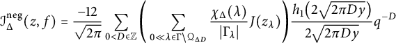 $$\begin{align*}\mathcal{I}^{\mathrm{neg}}_{\Delta}(z,f)=\frac{-12}{\sqrt{2\pi}}\sum_{0<D\in\mathbb{Z}}\Bigg(\sum_{0\ll \lambda\in\Gamma\backslash\mathcal{Q}_{\Delta D}}\frac{\chi_{\Delta}(\lambda)}{|\Gamma_{\lambda}|}J(z_{\lambda})\Bigg)\frac{h_{1}\big(2\sqrt{2\pi Dy}\big)}{2\sqrt{2\pi Dy}}q^{-D} \end{align*}$$
as well as
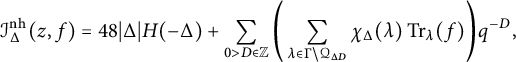 $$\begin{align*}\mathcal{I}^{\mathrm{nh}}_{\Delta}(z,f)=48|\Delta|H(-\Delta)+\sum_{0>D\in\mathbb{Z}}\Bigg(\sum_{\lambda\in\Gamma\backslash\mathcal{Q}_{\Delta D}}\chi_{\Delta}(\lambda)\operatorname{Tr}_{\lambda}(f)\Bigg)q^{-D}, \end{align*}$$
where for the latter constant we use equation (4.16) and the equality
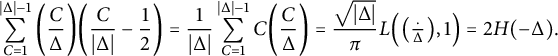 $$\begin{align*}\sum_{C=1}^{|\Delta|-1}\bigg(\frac{C}{\Delta}\bigg)\bigg(\frac{C}{|\Delta|}-\frac{1}{2}\bigg)=\frac{1}{|\Delta|}\sum_{C=1}^{|\Delta|-1}C\bigg(\frac{C}{\Delta}\bigg)=\frac{\sqrt{|\Delta|}}{\pi} L\Big(\big(\tfrac{\cdot}{\Delta}\big),1\Big)=2H(-\Delta). \end{align*}$$
Moreover, the congruence from equation (4.9) gives $a|\Delta $
, the fundamentality of
$a|\Delta $
, the fundamentality of $\Delta $
leaves only
$\Delta $
leaves only $a=|\Delta |$
after
$a=|\Delta |$
after $\Upsilon _{\Delta }$
, and then equation (4.16) and a standard Gauss sum evaluation yield
$\Upsilon _{\Delta }$
, and then equation (4.16) and a standard Gauss sum evaluation yield $\mathcal {I}^{\mathrm {c}}_{\Delta }(z,f)=\frac {12}{\sqrt {2\pi }}\sqrt {|\Delta |}\cdot \frac {J_{1}\big (2\sqrt {2\pi |\Delta |y}\big )}{2\sqrt {2\pi |\Delta |y}}q^{|\Delta |}$
.
$\mathcal {I}^{\mathrm {c}}_{\Delta }(z,f)=\frac {12}{\sqrt {2\pi }}\sqrt {|\Delta |}\cdot \frac {J_{1}\big (2\sqrt {2\pi |\Delta |y}\big )}{2\sqrt {2\pi |\Delta |y}}q^{|\Delta |}$
.
Now, let $\tilde {f}_{-\Delta }(z)$
denote the holomorphic part
$\tilde {f}_{-\Delta }(z)$
denote the holomorphic part $\mathcal {I}^{\mathrm {nh}}_{\Delta }(z,f)$
, which has the required expansion. Since Lemma 3.16 and equation (3.32) imply that
$\mathcal {I}^{\mathrm {nh}}_{\Delta }(z,f)$
, which has the required expansion. Since Lemma 3.16 and equation (3.32) imply that $\xi _{\frac {3}{2}}$
takes the functions
$\xi _{\frac {3}{2}}$
takes the functions $\frac {h_{1}(2\sqrt {2\pi Dy})}{(2\sqrt {2\pi Dy})}q^{-D}$
and
$\frac {h_{1}(2\sqrt {2\pi Dy})}{(2\sqrt {2\pi Dy})}q^{-D}$
and $\frac {J_{1}\big (2\sqrt {2\pi |\Delta |y}\big )}{2\sqrt {2\pi |\Delta |y}}q^{|\Delta |}$
to
$\frac {J_{1}\big (2\sqrt {2\pi |\Delta |y}\big )}{2\sqrt {2\pi |\Delta |y}}q^{|\Delta |}$
to $-\frac {q^{D}}{4\sqrt {2\pi D}}$
and
$-\frac {q^{D}}{4\sqrt {2\pi D}}$
and $+\frac {q^{\Delta }}{4\sqrt {2\pi |\Delta |}}$
respectively, the complement
$+\frac {q^{\Delta }}{4\sqrt {2\pi |\Delta |}}$
respectively, the complement $\mathcal {I}^{\mathrm {neg}}_{\Delta }(z,f)+\mathcal {I}^{\mathrm {c}}_{\Delta }(z,f)$
of
$\mathcal {I}^{\mathrm {neg}}_{\Delta }(z,f)+\mathcal {I}^{\mathrm {c}}_{\Delta }(z,f)$
of $\tilde {f}_{-\Delta }(z)$
is indeed harmonic, with the asserted
$\tilde {f}_{-\Delta }(z)$
is indeed harmonic, with the asserted $\xi _{\frac {3}{2}}$
-image
$\xi _{\frac {3}{2}}$
-image $\frac {3}{2\pi }f_{-\Delta }$
. This completes the proof of the theorem.
$\frac {3}{2\pi }f_{-\Delta }$
. This completes the proof of the theorem.
Proof of Theorem 1.2
We apply Theorem 4.3 to the lattice L in equation (2.8), where for which the parameters are $N=\alpha _{\ell }=\beta _{\ell }=\varepsilon _{\ell }=1$
, combined with the isomorphism from [Reference KohnenK] to scalar-valued modular forms. The vanishing of
$N=\alpha _{\ell }=\beta _{\ell }=\varepsilon _{\ell }=1$
, combined with the isomorphism from [Reference KohnenK] to scalar-valued modular forms. The vanishing of $c(0,k)$
implies the vanishing of the main terms of
$c(0,k)$
implies the vanishing of the main terms of $\mathcal {I}^{\mathrm {cc}}_{k,L}$
. As equations (3.10) and (3.41) evaluate the remaining term from equation (4.11) to be the asserted one, and the first term in equation (4.11) produces the one mentioned in Remark 1.3, this proves the first claim of the (extended) theorem. The remaining two claims follow directly from Corollary 4.4 (there exists only one cusp, so
$\mathcal {I}^{\mathrm {cc}}_{k,L}$
. As equations (3.10) and (3.41) evaluate the remaining term from equation (4.11) to be the asserted one, and the first term in equation (4.11) produces the one mentioned in Remark 1.3, this proves the first claim of the (extended) theorem. The remaining two claims follow directly from Corollary 4.4 (there exists only one cusp, so $c(0,k-1)=0$
in this case) and Proposition 4.5. This proves the theorem.
$c(0,k-1)=0$
in this case) and Proposition 4.5. This proves the theorem.
Remark 4.7 Using [Reference ZemelZe3, Reference ZemelZe7], the sum $\sum _{a=0}^{\lfloor p/2 \rfloor }\frac {1}{v^{a}a!}L_{\tau }^{a}\mathcal {I}_{k,L}(\tau ,f)$
is a (vector-valued) quasi-modular form of weight
$\sum _{a=0}^{\lfloor p/2 \rfloor }\frac {1}{v^{a}a!}L_{\tau }^{a}\mathcal {I}_{k,L}(\tau ,f)$
is a (vector-valued) quasi-modular form of weight $k+\frac {1}{2}$
and depth
$k+\frac {1}{2}$
and depth $\big \lfloor \frac {p}{2}\big \rfloor $
, and one checks that the contribution of
$\big \lfloor \frac {p}{2}\big \rfloor $
, and one checks that the contribution of $\mathcal {I}^{\mathrm {nh}}_{k,L,h}(\tau ,f)$
is just
$\mathcal {I}^{\mathrm {nh}}_{k,L,h}(\tau ,f)$
is just $\sum _{0 \leq m\in \mathbb {Z}+Q(h)}\operatorname {Tr}_{m,h}(f)q_{\tau }^{m}$
for every
$\sum _{0 \leq m\in \mathbb {Z}+Q(h)}\operatorname {Tr}_{m,h}(f)q_{\tau }^{m}$
for every $h \in D_{L}$
. Moreover, Lemmas 3.16 and 3.21 and equation (3.32) show that applying this combination to
$h \in D_{L}$
. Moreover, Lemmas 3.16 and 3.21 and equation (3.32) show that applying this combination to $\mathcal {I}^{\mathrm {neg}}_{k,L,h}(\tau ,f)$
,
$\mathcal {I}^{\mathrm {neg}}_{k,L,h}(\tau ,f)$
, $\mathcal {I}^{\mathrm {c}}_{k,L,h}(\tau ,f)$
, and
$\mathcal {I}^{\mathrm {c}}_{k,L,h}(\tau ,f)$
, and $\mathcal {I}^{\mathrm {cc}}_{k,L,h}(\tau ,f)$
amounts to replacing
$\mathcal {I}^{\mathrm {cc}}_{k,L,h}(\tau ,f)$
amounts to replacing $h_{l}$
from equation (4.13),
$h_{l}$
from equation (4.13), $J_{l}$
in equation (4.9), and
$J_{l}$
in equation (4.9), and $I_{k}$
appearing in equation (4.10) by
$I_{k}$
appearing in equation (4.10) by $\sum _{a}h_{l-2a}{(-2)^{a}a!}$
,
$\sum _{a}h_{l-2a}{(-2)^{a}a!}$
, $\sum _{a}J_{l-2a}{2^{a}a!}$
, and
$\sum _{a}J_{l-2a}{2^{a}a!}$
, and $\sum _{a}I_{k-2a}{2^{a}a!}$
, respectively. Moreover, after substituting equations (3.17), (3.31), and (3.29), the respective coefficient of
$\sum _{a}I_{k-2a}{2^{a}a!}$
, respectively. Moreover, after substituting equations (3.17), (3.31), and (3.29), the respective coefficient of $h_{0}$
,
$h_{0}$
, $J_{0}$
, and
$J_{0}$
, and $I_{0}$
in these combinations is just the corresponding denominator
$I_{0}$
in these combinations is just the corresponding denominator $\eta ^{l}$
or
$\eta ^{l}$
or $\eta ^{k}$
. It would be interesting to investigate these functions further. We also note that as long as
$\eta ^{k}$
. It would be interesting to investigate these functions further. We also note that as long as $2a \leq k$
, the term
$2a \leq k$
, the term $L_{\tau }^{a}\mathcal {I}_{k,L}(\tau ,f)$
is easily verified to be
$L_{\tau }^{a}\mathcal {I}_{k,L}(\tau ,f)$
is easily verified to be $\frac {1}{(-4\pi )^{a}}$
times the Shintani lift
$\frac {1}{(-4\pi )^{a}}$
times the Shintani lift $\mathcal {I}_{k-2a,L}(\tau ,L_{z}^{2a}f)$
.
$\mathcal {I}_{k-2a,L}(\tau ,L_{z}^{2a}f)$
.
4.3 Orbital integrals
In order to prove Theorem 4.3, we need to evaluate equation (4.15), which we can do for every $m\in \mathbb {Z}+Q(h)$
separately. Moreover, the integral over
$m\in \mathbb {Z}+Q(h)$
separately. Moreover, the integral over $Y_{T}$
can be replaced by an integral over
$Y_{T}$
can be replaced by an integral over $\mathcal {F}_{T}$
from equation (2.14), and integrals over (nice) regions in
$\mathcal {F}_{T}$
from equation (2.14), and integrals over (nice) regions in $\mathcal {H}$
can be expressed using the following lemma.
$\mathcal {H}$
can be expressed using the following lemma.
Lemma 4.8 Let $\lambda \in V_{\mathbb {R}}$
and
$\lambda \in V_{\mathbb {R}}$
and $f\in \widetilde {M}^{!}_{2k}(\Gamma )$
of some depth p be given, and take a connected domain
$f\in \widetilde {M}^{!}_{2k}(\Gamma )$
of some depth p be given, and take a connected domain $\mathcal {R}\subseteq \mathcal {H}$
with a piecewise smooth positively oriented boundary
$\mathcal {R}\subseteq \mathcal {H}$
with a piecewise smooth positively oriented boundary $\partial \mathcal {R}$
. Then we have
$\partial \mathcal {R}$
. Then we have
 $$\begin{align*}\int_{\mathcal{R}}f(z)\varphi_{k,-1}\big(\sqrt{v}\lambda,z\big)d\mu(z)=\sum_{\nu=0}^{p}\oint_{\partial\mathcal{R}}(L_{z}^{\nu}f)(z)\varphi_{k-\nu-1,\nu}\big(\sqrt{v}\lambda,z\big)dz.\end{align*}$$
Proof We apply Lemma 2.3 repeatedly, where in the $\nu $
th step f is replaced by
$\nu $
th step f is replaced by $L_{z}^{\nu }f$
and
$L_{z}^{\nu }f$
and $g(z)=\varphi _{k-\nu ,\nu -1}\big (\sqrt {v}\lambda ,z\big )$
. Then Proposition 3.18 allows us to take
$g(z)=\varphi _{k-\nu ,\nu -1}\big (\sqrt {v}\lambda ,z\big )$
. Then Proposition 3.18 allows us to take $G(z)=\varphi _{k-\nu -1,\nu }\big (\sqrt {v}\lambda ,z\big )$
, and the sum ends after
$G(z)=\varphi _{k-\nu -1,\nu }\big (\sqrt {v}\lambda ,z\big )$
, and the sum ends after $\nu =p$
since
$\nu =p$
since $L_{z}^{p+1}f=0$
by assumption. This proves the lemma.
$L_{z}^{p+1}f=0$
by assumption. This proves the lemma.
In view of equation (4.12), we will need the following lemma later.
Lemma 4.9 Let $\lambda \in V$
with
$\lambda \in V$
with $\iota (\lambda )=1$
,
$\iota (\lambda )=1$
, $v>0$
, and
$v>0$
, and $f\in \widetilde {M}^{!}_{2k}(\Gamma )$
of some depth p be given, and denote
$f\in \widetilde {M}^{!}_{2k}(\Gamma )$
of some depth p be given, and denote $\eta =2\sqrt {2\pi Q(\lambda )v}$
. Then we have the equality
$\eta =2\sqrt {2\pi Q(\lambda )v}$
. Then we have the equality
 $$\begin{align*}\sum_{b=0}^{\lfloor p/2 \rfloor}\frac{\operatorname{Sing}_{\lambda}(L_{z}^{2b}f)}{(4\pi v)^{b}b!}=i^{k}\big(2\sqrt{Q(\lambda)}\big)^{k-1}\sum_{n\in\mathbb{Z}}\sum_{l=0}^{p}c_{\ell_{\lambda}}(n,l)\mathbf{e}\bigg(\frac{nr_{\lambda}}{\alpha_{\ell_{\lambda}}}\bigg) \phi_{n}\bigg(k-l,T;\frac{2\pi}{\alpha_{\ell_{\lambda}}}\bigg)\frac{\operatorname{He}_{l}(\eta)}{\eta^{l}}.\end{align*}$$
Proof As Corollary 3.7 presents the coefficient in front of $\operatorname {Sing}_{\lambda }(L_{z}^{\mu }f)$
on the left-hand side of the first equality as
$\operatorname {Sing}_{\lambda }(L_{z}^{\mu }f)$
on the left-hand side of the first equality as $\frac {P_{\mu }(0)}{(2\pi v)^{\mu /2}}$
, substituting equation (4.5), with the summation index l replacing
$\frac {P_{\mu }(0)}{(2\pi v)^{\mu /2}}$
, substituting equation (4.5), with the summation index l replacing $l-\mu $
, into equation (4.4), expresses the left-hand side of the first equality as
$l-\mu $
, into equation (4.4), expresses the left-hand side of the first equality as
 $$ \begin{align*} &\sum_{\mu=0}^{p}\frac{P_{\mu}(0)}{(2\pi v)^{\mu/2}}i^{k-\mu}(2\sqrt{Q(\lambda)})^{k-\mu-1}\sum_{l=\mu}^{p}\sum_{n\in\mathbb{Z}}\frac{l!c_{\ell_{\lambda}}(n,l)}{(l-\mu)!}\mathbf{e}\bigg(\frac{nr_{\lambda}}{\alpha_{\ell_{\lambda}}}\bigg) \phi_{n}\bigg((k-\mu)-(l-\mu),T;\frac{2\pi}{\alpha_{\ell_{\lambda}}}\bigg) \\ &=i^{k}(2\sqrt{Q(\lambda)})^{k-1}\sum_{j=0}^{p}\sum_{n\in\mathbb{Z}}c_{\ell_{\lambda}}(n,l)\mathbf{e}\bigg(\frac{nr_{\lambda}}{\alpha_{\ell_{\lambda}}}\bigg)\phi_{n}\bigg(k-l,T;\frac{2\pi}{\alpha_{\ell_{\lambda}}}\bigg) \sum_{\mu=0}^{l}\frac{l!P_{\mu}(0)}{(l-\mu)!(2i\sqrt{2\pi Q(\lambda)v})^{\mu}}. \end{align*} $$
Equation (3.11) and Corollary 3.7 now express the sum over $\mu $
as
$\mu $
as $\frac {l!P_{l}(i\eta )}{(i\eta )^{l}}=\frac {\operatorname {He}_{l}(\eta )}{\eta ^{l}}$
, as desired. This proves the lemma.
$\frac {l!P_{l}(i\eta )}{(i\eta )^{l}}=\frac {\operatorname {He}_{l}(\eta )}{\eta ^{l}}$
, as desired. This proves the lemma.
Now, the coefficient of $q^{m}$
in equation (4.15) is evaluated for
$q^{m}$
in equation (4.15) is evaluated for $m<0$
,
$m<0$
, $m>0$
with
$m>0$
with $\iota (m)=0$
,
$\iota (m)=0$
, $m>0$
with
$m>0$
with $\iota (m)=1$
, and
$\iota (m)=1$
, and $m=0$
respectively, in the following four propositions.
$m=0$
respectively, in the following four propositions.
Proposition 4.10 For every $h \in D_{L}$
and
$h \in D_{L}$
and $0>m\in \mathbb {Z}+Q(h)$
, we have the equality
$0>m\in \mathbb {Z}+Q(h)$
, we have the equality
 $$\begin{align*}&\lim_{T\to\infty}\!v^{\frac{1-k}{2}}\!\int_{Y_{T}}\!\!f(z)\!\!\sum_{\lambda \in L_{m,h}}\!\!\varphi_{k,-1}\big(\sqrt{v}\lambda,z\big)d\mu(z)\\ & \quad = \sum_{l=k}^{p}\!\frac{4^{k}\sqrt{\pi}|m|^{\frac{k-1}{2}}h_{l}(2\sqrt{2\pi|m|v})\operatorname{Tr}_{m,h}^{(k)}(R_{2k-2l}^{l-k}L_{z}^{l}f)}{\sqrt{2}(4\sqrt{2\pi|m|v})^{l}(l-k)!}.\end{align*}$$
Proof The proof is similar to that of Proposition 3.9 of [Reference Bruinier, Funke, Imamoğlu and LiBFIL]. Remark 3.15 gives us the strong decay of $\varphi _{\kappa ,\nu }\big (\sqrt {v}\lambda ,z\big )$
, so that we can take the integral over
$\varphi _{\kappa ,\nu }\big (\sqrt {v}\lambda ,z\big )$
, so that we can take the integral over $z \in Y$
. Unfolding, cutting out a small neighborhood
$z \in Y$
. Unfolding, cutting out a small neighborhood $B_{\epsilon }(z_{\lambda })$
for each
$B_{\epsilon }(z_{\lambda })$
for each $\lambda \in \Gamma \backslash L_{m,h}$
, and applying Lemma 4.8 yields
$\lambda \in \Gamma \backslash L_{m,h}$
, and applying Lemma 4.8 yields
 $$\begin{align*}&\int_{Y}f(z)\sum_{\lambda \in L_{m,h}}\varphi_{k,-1}\big(\sqrt{v}\lambda,z\big)d\mu(z)\\ & \quad =\lim_{\epsilon\to0}\sum_{\lambda\in \Gamma \backslash L_{m,h}}\!\frac{-1}{|\Gamma_{\lambda}|}\sum_{l=0}^{p}\oint_{\partial B_{\epsilon}(z_{\lambda})}(L_{z}^{l}f)(z)\varphi_{k-1-l,l}\big(\sqrt{v}\lambda,z\big)dz.\end{align*}$$
Substituting equations (2.6) and (3.18) (with $\zeta =\sigma \sqrt {|m|}$
for
$\zeta =\sigma \sqrt {|m|}$
for $\sigma :=-\operatorname {sgn}\big (\lambda ,Z^{\perp }(z_{\lambda })\big )$
), and multiplying by
$\sigma :=-\operatorname {sgn}\big (\lambda ,Z^{\perp }(z_{\lambda })\big )$
), and multiplying by $v^{\frac {1-k}{2}}$
, shows that the desired left-hand side is the sum over
$v^{\frac {1-k}{2}}$
, shows that the desired left-hand side is the sum over $\lambda $
and l of
$\lambda $
and l of
 $$\begin{align*}\sum_{\lambda\in \Gamma \backslash L_{m,h}}\sum_{l=0}^{p}\frac{-\big(4y_{\lambda}\sigma\sqrt{|m|}\big)^{k-1-l}}{(2\pi)^{(l+1)/2}v^{l/2}|\Gamma_{\lambda}|}\lim_{\epsilon\to0}\oint_{\partial B_{\epsilon}(z_{\lambda})}\frac{(L_{z}^{l}f)(z)A_{z_{\lambda}}(z)^{k-1-l}dz}{\big(1-A_{z_{\lambda}}(z)\big)^{2k-2l-2}}h_{l}\big(2\sigma\sqrt{2\pi mv}\tfrac{1+\epsilon^{2}}{1-\epsilon^{2}}\big).\end{align*}$$
Evaluating this limit via Corollary 2.2, using the parity from Proposition 3.14, and applying equations (4.1) and (4.7) yields the desired right-hand side. This proves the proposition.
Proposition 4.11 If $h \in D_{L}$
and
$h \in D_{L}$
and $0<m\in \mathbb {Z}+Q(h)$
with
$0<m\in \mathbb {Z}+Q(h)$
with $\iota (m)=0$
, then we have
$\iota (m)=0$
, then we have
 $$\begin{align*}v^{\frac{1-k}{2}}\lim_{T\to\infty}\int_{Y_{T}}f(z)\sum_{\lambda \in L_{m,h}}\varphi_{k,-1}\big(\sqrt{v}\lambda,z\big)d\mu(z)=\sum_{b=0}^{\lfloor p/2 \rfloor}\frac{\operatorname{Tr}_{m,h}(L_{z}^{2b}f)}{(4\pi v)^{b}b!}.\end{align*}$$
Proof An element $\lambda \in L_{m,h}$
is not perpendicular to
$\lambda \in L_{m,h}$
is not perpendicular to $\ell $
for any
$\ell $
for any $\ell \in \operatorname {Iso}(V)$
, and its stabilizer
$\ell \in \operatorname {Iso}(V)$
, and its stabilizer $\Gamma _{\lambda }$
is infinite cyclic by Lemma 2.5. Therefore, the functions
$\Gamma _{\lambda }$
is infinite cyclic by Lemma 2.5. Therefore, the functions $\varphi _{\kappa ,\nu }\big (\sqrt {v}\lambda ,z\big )$
again decay strongly, via Remark 3.15, toward any cusp
$\varphi _{\kappa ,\nu }\big (\sqrt {v}\lambda ,z\big )$
again decay strongly, via Remark 3.15, toward any cusp $\ell $
. We combine this with the usual unfolding argument to express our left-hand side as
$\ell $
. We combine this with the usual unfolding argument to express our left-hand side as
 $$\begin{align*}&v^{\frac{1-k}{2}}\lim_{T\to\infty}\sum_{\lambda\in\Gamma \backslash L_{m,h}}\int_{\mathcal{F}_{\lambda,T}}f(z)\varphi_{k,-1}\big(\sqrt{v}\lambda,z\big)d\mu(z)\\&\quad =v^{\frac{1-k}{2}}\sum_{\lambda\in\Gamma \backslash L_{m,h}}\int_{\mathcal{F}_{\lambda}}f(z)\varphi_{k,-1}\big(\sqrt{v}\lambda,z\big)d\mu(z), \end{align*}$$
where $\mathcal {F}_{\lambda }$
is a fundamental domain for the action of
$\mathcal {F}_{\lambda }$
is a fundamental domain for the action of $\Gamma _{\lambda }$
on
$\Gamma _{\lambda }$
on $\mathcal {H}$
and
$\mathcal {H}$
and $\mathcal {F}_{\lambda ,T}:=\mathcal {F}_{\lambda }\cap \mathcal {H}_{T}$
(this is well defined modulo
$\mathcal {F}_{\lambda ,T}:=\mathcal {F}_{\lambda }\cap \mathcal {H}_{T}$
(this is well defined modulo $\Gamma $
by equation (3.20) and the modularity of f). We now remove an
$\Gamma $
by equation (3.20) and the modularity of f). We now remove an $\epsilon $
-neighborhood of the geodesic
$\epsilon $
-neighborhood of the geodesic $c_{\lambda }$
from
$c_{\lambda }$
from $\mathcal {F}_{\lambda }$
for applying Lemma 4.8, substitute the value of each
$\mathcal {F}_{\lambda }$
for applying Lemma 4.8, substitute the value of each $\varphi _{k-\nu -1,\nu }$
from equation (3.18), and gather powers of v to write our expression as
$\varphi _{k-\nu -1,\nu }$
from equation (3.18), and gather powers of v to write our expression as
 $$\begin{align*}-\sum_{\lambda\in\Gamma \backslash L_{m,h}} \sum_{\nu=0}^{p} \frac{\lim_{\epsilon\to 0^{+}} \big(h_{\nu}(\epsilon) - h_{\nu}(- \epsilon)\big)}{(2\pi)^{(\nu+1)/2}v^{\nu/2}} \int_{c_{\lambda}\cap \mathcal{F}_{\lambda}}(L_{z}^{\nu}f)(z)(\lambda,Z(z))^{k-\nu-1}dz. \end{align*}$$
However, the integral is $\operatorname {Tr}_{\lambda }(L_{z}^{\nu }f)$
from equation (4.2), summing over
$\operatorname {Tr}_{\lambda }(L_{z}^{\nu }f)$
from equation (4.2), summing over $\lambda $
replaces it by
$\lambda $
replaces it by $\operatorname {Tr}_{m,h}(L_{z}^{\nu }f)$
from equation (4.7), and we have
$\operatorname {Tr}_{m,h}(L_{z}^{\nu }f)$
from equation (4.7), and we have $\lim _{\epsilon \to 0^{+}}\big (h_{\nu }(\epsilon )-h_{\nu }(-\epsilon )\big )=-\sqrt {2\pi }P_{\nu }(0)$
by Proposition 3.14. The desired formula now follows from Corollary 3.7. This proves the proposition.
$\lim _{\epsilon \to 0^{+}}\big (h_{\nu }(\epsilon )-h_{\nu }(-\epsilon )\big )=-\sqrt {2\pi }P_{\nu }(0)$
by Proposition 3.14. The desired formula now follows from Corollary 3.7. This proves the proposition.
When $\iota (m)=1$
, the coefficient
$\iota (m)=1$
, the coefficient $a(\Theta _{k,\ell },m,h,v)$
from (2.23), as well as the traces from equations (4.9) and (4.10), may be nonzero. Recalling the functions
$a(\Theta _{k,\ell },m,h,v)$
from (2.23), as well as the traces from equations (4.9) and (4.10), may be nonzero. Recalling the functions $\phi _{n}$
from equation (4.4), the limit of the corresponding coefficient from equation (4.15) is evaluated as follows.
$\phi _{n}$
from equation (4.4), the limit of the corresponding coefficient from equation (4.15) is evaluated as follows.
Proposition 4.12 Let $h \in D_{L}$
and
$h \in D_{L}$
and $0<m\in \mathbb {Z}+Q(h)$
with
$0<m\in \mathbb {Z}+Q(h)$
with $\iota (m)=1$
be given. Then, for large
$\iota (m)=1$
be given. Then, for large $T>1$
, we have
$T>1$
, we have
 $$\begin{align*}\begin{aligned} v^{\frac{1-k}{2}}&\int_{Y_{T}}f(z)\sum_{\lambda \in L_{m,h}}\varphi_{k,-1}\big(\sqrt{v}\lambda,z\big)d\mu(z)=\sum_{b=0}^{\lfloor p/2 \rfloor}\frac{\operatorname{Tr}_{m,h}(L_{z}^{2b}f)}{(4\pi v)^{b}b!}+\operatorname{Tr}^{\mathrm{c}}_{m,h}(f,v) \\ &+\operatorname{Tr}^{\mathrm{cc}}_{m,h}(f,v)-\sum_{\ell\in\Gamma\backslash\operatorname{Iso}(V)}\frac{\varepsilon_{\ell}i^{k}}{\sqrt{N}}a(\Theta_{k,\ell},m,h,v)\sum_{l=0}^{p}c_{\ell}(0,l)\phi_{0}(k-l,T)+O\big(\tfrac{1}{T}\big). \end{aligned} \end{align*}$$
Proof For $\lambda \in L_{m,h}$
, we set
$\lambda \in L_{m,h}$
, we set $\mathcal {H}_{\lambda ,T}:=\mathcal {H}\setminus \big (B_{\epsilon }(\ell _{\lambda })\cup B_{\epsilon }(\ell _{-\lambda })\big )$
for
$\mathcal {H}_{\lambda ,T}:=\mathcal {H}\setminus \big (B_{\epsilon }(\ell _{\lambda })\cup B_{\epsilon }(\ell _{-\lambda })\big )$
for $\epsilon =e^{-2\pi T}$
. The usual unfolding argument, the fact that the stabilizer of
$\epsilon =e^{-2\pi T}$
. The usual unfolding argument, the fact that the stabilizer of $\lambda \in L_{m,h}$
is trivial by Lemma 2.5, and the decay from Remark 3.15 allow us to replace, as in Lemma 5.2 of [Reference Bruinier and FunkeBF2], the left-hand side by
$\lambda \in L_{m,h}$
is trivial by Lemma 2.5, and the decay from Remark 3.15 allow us to replace, as in Lemma 5.2 of [Reference Bruinier and FunkeBF2], the left-hand side by
 $$\begin{align*}&v^{\frac{1-k}{2}}\!\sum_{\lambda\in\Gamma \backslash L_{m,h}}\!\int_{H_{T}}f(z)\varphi_{k,-1}\big(\sqrt{v}\lambda,z\big)d\mu(z)\\& \quad =v^{\frac{1-k}{2}}\!\!\sum_{\lambda\in\Gamma \backslash L_{m,h}}\!\int_{H_{\lambda,T}}\!f(z)\varphi_{k,-1}\big(\sqrt{v}\lambda,z\big)d\mu(z)+O\big(\tfrac{1}{T}\big)\end{align*}$$
(the error term here is, in fact, much better). The argument from the proof of Proposition 4.11 expresses the term associated with $\lambda \in \Gamma \backslash L_{m,h}$
as
$\lambda \in \Gamma \backslash L_{m,h}$
as
 $$ \begin{align} &\sum_{b=0}^{\lfloor p/2 \rfloor}\frac{1}{(4\pi v)^{b}b!}\int_{c(\lambda) \cap Y_{T}}\!(L_{z}^{2b}f)(z)(\lambda,Z(z))^{k-1-2b}dz\\ & \quad +\sum_{\nu=0}^{p}v^{\frac{1-k}{2}}\int_{\partial \mathcal{H}_{\lambda,T}}\!(L_{z}^{\nu}f)(z)\varphi_{k-\nu-1,\nu}\big(\sqrt{v}\lambda,z\big)dz.\nonumber \end{align} $$
Next, $\partial \mathcal {H}_{\lambda ,T}=\partial B_{\epsilon }(\ell _{\lambda })\cup \partial B_{\epsilon }(\ell _{-\lambda })$
for this
$\partial \mathcal {H}_{\lambda ,T}=\partial B_{\epsilon }(\ell _{\lambda })\cup \partial B_{\epsilon }(\ell _{-\lambda })$
for this $\epsilon $
, both with the opposite orientation. In the integral along the first part, as
$\epsilon $
, both with the opposite orientation. In the integral along the first part, as $\sigma _{\ell }^{-1}$
takes
$\sigma _{\ell }^{-1}$
takes $\partial B_{\epsilon }(\ell _{\lambda })$
to
$\partial B_{\epsilon }(\ell _{\lambda })$
to $\mathbb {R}+iT$
, equation (2.17) expresses the corresponding term in equation (4.17) as
$\mathbb {R}+iT$
, equation (2.17) expresses the corresponding term in equation (4.17) as
 $$\begin{align*}-\sum_{\nu=0}^{p} \int_{-\infty}^{\infty} v^{\frac{1-k}{2}} (L_{z}^{\nu} f|_{2k-2\nu} \sigma_{\ell_{\lambda}}) (x_{\ell_{\lambda}}+iT)\varphi_{k-\nu-1,\nu}\bigg(\sqrt{\tfrac{mv}{N}}\big(\begin{smallmatrix} 1 & -2r_{\lambda} \\ 0 &-1\end{smallmatrix}\big),x_{\ell_{\lambda}}+iT\bigg)dx_{\ell_{\lambda}}. \end{align*}$$
Equation (3.19) thus implies that the integral along $\partial B_{\epsilon }(\ell _{-\lambda })$
is evaluated in the same manner, with
$\partial B_{\epsilon }(\ell _{-\lambda })$
is evaluated in the same manner, with $\lambda $
replaced by
$\lambda $
replaced by $-\lambda $
, and multiplied by
$-\lambda $
, and multiplied by $(-1)^{k}$
.
$(-1)^{k}$
.
Applying equation (3.18), noting that the pairings with $Z(x_{\ell _{\lambda }}+iT)$
and
$Z(x_{\ell _{\lambda }}+iT)$
and $Z^{\perp }(x_{\ell _{\lambda }}+iT)$
are
$Z^{\perp }(x_{\ell _{\lambda }}+iT)$
are $2\sqrt {mv}(x_{\ell _{\lambda }}+iT-r_{\lambda })$
and
$2\sqrt {mv}(x_{\ell _{\lambda }}+iT-r_{\lambda })$
and $\frac {2\sqrt {mv}}{T}(x_{\ell _{\lambda }}-r_{\lambda })$
respectively, we substitute
$\frac {2\sqrt {mv}}{T}(x_{\ell _{\lambda }}-r_{\lambda })$
respectively, we substitute $\eta :=2\sqrt {2\pi mv}$
and
$\eta :=2\sqrt {2\pi mv}$
and $\xi :=\frac {\eta }{T}(x_{\ell _{\lambda }}-r_{\lambda })$
and use equations (4.5) and (3.24) and the definition of the Fourier transform to present the latter expression as
$\xi :=\frac {\eta }{T}(x_{\ell _{\lambda }}-r_{\lambda })$
and use equations (4.5) and (3.24) and the definition of the Fourier transform to present the latter expression as
 $$ \begin{align*} -&v^{\frac{1-k}{2}}\sum_{\nu=0}^{p}\int_{-\infty}^{\infty}\sum_{n\in\mathbb{Z}}\sum_{l=\nu}^{p}\frac{(-1)^{\nu}l!c_{\ell_{\lambda}}(n,l)}{(l-\nu)!T^{l-\nu}}e^{-2\pi nT/\alpha_{\ell_{\lambda}}}\mathbf{e}\Big(\tfrac{nx_{\ell_{\lambda}}}{\alpha_{\ell_{\lambda}}}\Big)\frac{T^{k-\nu-1}}{(2\pi)^{k/2}}(\xi+i\eta)^{k-\nu-1}h_{\nu}(\xi)dx_{\ell_{\lambda}} \\ =&-v^{\frac{1-k}{2}}\sum_{n\in\mathbb{Z}}\sum_{l=0}^{p}\frac{l!c_{\ell_{\lambda}}(n,l)T^{k-l-1}}{(2\pi)^{k/2}}e^{-2\pi nT/\alpha_{\ell_{\lambda}}}\int_{-\infty}^{\infty}\mathbf{e}\Big(\tfrac{nx_{\ell_{\lambda}}}{\alpha_{\ell_{\lambda}}}\Big)\mathbf{g}_{k-l,l}(\xi;\eta)dx_{\ell_{\lambda}} \\ =&-v^{\frac{1-k}{2}}\sum_{n\in\mathbb{Z}}\sum_{l=0}^{p}\frac{l!c_{\ell_{\lambda}}(n,l)T^{k-l}}{(2\pi)^{k/2}\eta}e^{-2\pi nT/\alpha_{\ell_{\lambda}}}\mathbf{e}\Big(\tfrac{nr_{\lambda}}{\alpha_{\ell_{\lambda}}}\Big)\widehat{\mathbf{g}_{k-l,l}}\Big(-\tfrac{nT}{\alpha_{\ell_{\lambda}}\eta};\eta\Big). \end{align*} $$
Propositions 3.22 and 3.25 show, via equation (4.4), that the contribution of fixed n and l to the latter expression is $\frac {i^{k}\eta ^{k-1}}{(2\pi v)^{(k-1)/2}}c_{\ell _{\lambda }}(n,l)\mathbf {e}\big (\frac {nr_{\lambda }}{\alpha _{\ell _{\lambda }}}\big )=i^{k}\big (2\sqrt {m}\big )^{k-1}c_{\ell _{\lambda }}(n,l)\mathbf {e}\big (\frac {nr_{\lambda }}{\alpha _{\ell _{\lambda }}}\big )$
times
$\frac {i^{k}\eta ^{k-1}}{(2\pi v)^{(k-1)/2}}c_{\ell _{\lambda }}(n,l)\mathbf {e}\big (\frac {nr_{\lambda }}{\alpha _{\ell _{\lambda }}}\big )=i^{k}\big (2\sqrt {m}\big )^{k-1}c_{\ell _{\lambda }}(n,l)\mathbf {e}\big (\frac {nr_{\lambda }}{\alpha _{\ell _{\lambda }}}\big )$
times
 $$\begin{align*}\begin{cases} \frac{\operatorname{He}_{l}(\eta)}{\eta^{l}}\phi_{n}\Big(k-l,T;\frac{2\pi}{\alpha_{\ell_{\lambda}}}\Big), & n>0\text{ or }n<0\text{ and }l>k, \\[3pt] \frac{\operatorname{He}_{l}(\eta)}{\eta^{l}}\phi_{n}\Big(k-l,T;\frac{2\pi}{\alpha_{\ell_{\lambda}}}\Big)-(-1)^{k}\sqrt{2\pi}\big(\frac{2\pi n}{\alpha_{\ell_{\lambda}}}\big)^{l-k}\frac{l!}{(l-k)!}\frac{J_{l}(\eta)}{\eta^{l}}, & n<0\text{ and }l \geq k, \\[3pt] \big(\frac{\operatorname{He}_{l}(\eta)}{\eta^{l}}-\frac{\operatorname{He}_{k}(\eta)}{\eta^{k}}\big)\phi_{0}(k-l,T), & n=0\text{ and }l \neq k, \\[3pt] \big(\frac{\operatorname{He}_{l}(\eta)}{\eta^{l}}-\frac{\operatorname{He}_{k}(\eta)}{\eta^{k}}\big)\phi_{0}(k-l,T)-\frac{(-1)^{k}k!}{\eta^{k}}\big(I_{k}(\eta)-\tilde{\Omega}_{k}(\eta)\big), & n=0\text{ and }l=k, \\ \end{cases}\end{align*}$$
where the error terms from the former proposition go into $O\big (\frac {1}{T}\big )$
and the first term with
$O\big (\frac {1}{T}\big )$
and the first term with $l=k$
trivially vanishes.
$l=k$
trivially vanishes.
Now, since $Q(\lambda )=m$
for our
$Q(\lambda )=m$
for our $\lambda $
, Lemma 4.9 shows that the sum over n and l of the first terms gives
$\lambda $
, Lemma 4.9 shows that the sum over n and l of the first terms gives $\sum _{b=0}^{\lfloor p/2 \rfloor }\frac {\operatorname {Sing}_{\lambda }(L_{z}^{2b}f)}{(4\pi v)^{b}b!}$
. Hence, these terms, the corresponding ones from the integral along
$\sum _{b=0}^{\lfloor p/2 \rfloor }\frac {\operatorname {Sing}_{\lambda }(L_{z}^{2b}f)}{(4\pi v)^{b}b!}$
. Hence, these terms, the corresponding ones from the integral along $\partial B_{\epsilon }(\ell _{-\lambda })$
, and the first term from equation (4.17) combine, via equation (4.6), to
$\partial B_{\epsilon }(\ell _{-\lambda })$
, and the first term from equation (4.17) combine, via equation (4.6), to $\sum _{b=0}^{\lfloor p/2 \rfloor }\frac {\operatorname {Tr}_{\lambda }(L_{z}^{2b}f)}{(4\pi v)^{b}b!}$
, and after summing over all
$\sum _{b=0}^{\lfloor p/2 \rfloor }\frac {\operatorname {Tr}_{\lambda }(L_{z}^{2b}f)}{(4\pi v)^{b}b!}$
, and after summing over all $\lambda \in \Gamma \backslash L_{m,h}$
, we get the first asserted term by equation (4.7). Now, fix
$\lambda \in \Gamma \backslash L_{m,h}$
, we get the first asserted term by equation (4.7). Now, fix $\ell \in \Gamma \backslash \operatorname {Iso}(V)$
, and equation (2.18) implies that in the sum of the remaining terms over
$\ell \in \Gamma \backslash \operatorname {Iso}(V)$
, and equation (2.18) implies that in the sum of the remaining terms over $\lambda \in \Gamma \backslash L_{m,h}$
, we only get contributions to the integral along
$\lambda \in \Gamma \backslash L_{m,h}$
, we only get contributions to the integral along $\partial B_{\epsilon }(\ell _{\lambda })$
when
$\partial B_{\epsilon }(\ell _{\lambda })$
when $\iota _{\ell }(m,h)=1$
, and to the one over
$\iota _{\ell }(m,h)=1$
, and to the one over $\partial B_{\epsilon }(\ell _{-\lambda })$
if
$\partial B_{\epsilon }(\ell _{-\lambda })$
if $\iota _{\ell }(m,-h)=1$
, with the sign
$\iota _{\ell }(m,-h)=1$
, with the sign $(-1)^{k}$
. Lemma 2.6 and Remark 2.7 now imply that, for such
$(-1)^{k}$
. Lemma 2.6 and Remark 2.7 now imply that, for such $\ell $
, the sum of
$\ell $
, the sum of $\mathbf {e}\big (\frac {nr_{\lambda }}{\alpha _{\ell _{\lambda }}}\big )$
over
$\mathbf {e}\big (\frac {nr_{\lambda }}{\alpha _{\ell _{\lambda }}}\big )$
over $\lambda $
with
$\lambda $
with $\ell _{\lambda }=\ell $
gives
$\ell _{\lambda }=\ell $
gives $2\varepsilon _{\ell }\sqrt {\frac {m}{N}}\mathbf {e}\big (\frac {nr_{\lambda }}{\alpha _{\ell _{\lambda }}}\big )$
in case
$2\varepsilon _{\ell }\sqrt {\frac {m}{N}}\mathbf {e}\big (\frac {nr_{\lambda }}{\alpha _{\ell _{\lambda }}}\big )$
in case $2\varepsilon _{\ell }\sqrt {\frac {m}{N}}$
divides n and 0 otherwise. The resulting sums thus produce the remaining required terms by equations (4.9), (4.10), and (2.23) and the value of
$2\varepsilon _{\ell }\sqrt {\frac {m}{N}}$
divides n and 0 otherwise. The resulting sums thus produce the remaining required terms by equations (4.9), (4.10), and (2.23) and the value of $\eta $
. This completes the proof of the proposition.
$\eta $
. This completes the proof of the proposition.
The proof of Proposition 4.12 also shows that the regularized traces that show up in that proposition, interpreted as regularized L-values, are not those of $L_{z}^{2b}f$
but rather of its image under the Hecke U-operator of index
$L_{z}^{2b}f$
but rather of its image under the Hecke U-operator of index $2\varepsilon _{\ell }\sqrt {\frac {m}{N}}$
.
$2\varepsilon _{\ell }\sqrt {\frac {m}{N}}$
.
We can now state and prove the analog of Propositions 4.10–4.12 for $m=0$
, again using the expressions from equations (2.23) and (4.4), and with the trace from equation (4.11).
$m=0$
, again using the expressions from equations (2.23) and (4.4), and with the trace from equation (4.11).
Proposition 4.13 For an isotropic element $h \in D_{L}$
and large
$h \in D_{L}$
and large $T>1$
, we have
$T>1$
, we have
 $$\begin{align*}\begin{aligned} v^{\frac{1-k}{2}}\int_{Y_{T}}&f(z)\sum_{\lambda \in L_{0,h}}\varphi_{k,-1}\big(\sqrt{v}\lambda,z\big)d\mu(z)=\sum_{b=0}^{\lfloor p/2 \rfloor}\frac{\operatorname{Tr}_{0,h}(L_{z}^{2b}f)}{(4\pi v)^{b}b!}+\operatorname{Tr}^{\mathrm{cc}}_{0,h}(f,v) \\ &-\sum_{\ell\in\Gamma\backslash\operatorname{Iso}(V)}\frac{i^{k}\varepsilon_{\ell}}{\sqrt{N}}a(\Theta_{k,\ell},0,h,v)\sum_{l=0}^{p}c_{\ell}(0,l)\phi_{0}(k-l,T)+O\big(\tfrac{1}{T}\big). \end{aligned} \end{align*}$$
Proof It is easy to see that $L_{0,h}\setminus \{0\}=\bigcup _{\{\ell \in \operatorname {Iso}(V)\,|\,\iota _{\ell }(0,h)=1\}}[(L+h)\cap \ell ]$
, a union that respects the
$L_{0,h}\setminus \{0\}=\bigcup _{\{\ell \in \operatorname {Iso}(V)\,|\,\iota _{\ell }(0,h)=1\}}[(L+h)\cap \ell ]$
, a union that respects the $\Gamma $
-action. The same unfolding argument from the proofs of Propositions 4.11 and 4.12 allows us to write this part of the left-hand side as
$\Gamma $
-action. The same unfolding argument from the proofs of Propositions 4.11 and 4.12 allows us to write this part of the left-hand side as
 $$\begin{align*}\sum_{\{\ell\in\Gamma\backslash\operatorname{Iso}(V)\,|\,\iota_{\ell}(0,h)=1\}}v^{\frac{1-k}{2}}\int_{\Gamma_{\ell}\backslash\mathcal{H}_{T}}f(z)\sum_{\lambda \in (L+h)\cap\ell}\varphi_{k,-1}\big(\sqrt{v}\lambda,z\big)d\mu(z), \end{align*}$$
and Remark 3.15 implies that replacing $\Gamma _{\ell }\backslash \mathcal {H}_{T}$
by
$\Gamma _{\ell }\backslash \mathcal {H}_{T}$
by $\Gamma _{\ell }\backslash \mathcal {H}_{\ell ,T}$
, for
$\Gamma _{\ell }\backslash \mathcal {H}_{\ell ,T}$
, for $\mathcal {H}_{\ell ,T}:=\mathcal {H}_{T} \setminus B_{\epsilon }(\ell )$
, produces an error term that is much smaller that
$\mathcal {H}_{\ell ,T}:=\mathcal {H}_{T} \setminus B_{\epsilon }(\ell )$
, produces an error term that is much smaller that $O\big (\frac {1}{T}\big )$
Footnote
6
. As
$O\big (\frac {1}{T}\big )$
Footnote
6
. As $\ell $
is perpendicular to neither
$\ell $
is perpendicular to neither $Z(z)$
nor
$Z(z)$
nor $Z^{\perp }(z)$
for any
$Z^{\perp }(z)$
for any $z\in \mathcal {H}$
, when we invoke Lemma 4.8 as the proof of Proposition 4.12, only the (negatively oriented) integral along the boundary
$z\in \mathcal {H}$
, when we invoke Lemma 4.8 as the proof of Proposition 4.12, only the (negatively oriented) integral along the boundary $\Gamma _{\ell }\backslash \partial B_{\epsilon }(\ell )$
remains. Now, since equation (2.9) shows that the latter maps under
$\Gamma _{\ell }\backslash \partial B_{\epsilon }(\ell )$
remains. Now, since equation (2.9) shows that the latter maps under $\sigma _{\ell }^{-1}$
onto
$\sigma _{\ell }^{-1}$
onto $(\mathbb {R}/\alpha _{\ell }\mathbb {Z})+iT$
, equation (2.11) expresses the summand associated with
$(\mathbb {R}/\alpha _{\ell }\mathbb {Z})+iT$
, equation (2.11) expresses the summand associated with $\ell $
as
$\ell $
as
 $$\begin{align*}-\sum_{\nu=0}^{p}v^{\frac{1-k}{2}}\!\int_{\mathbb{R}/\alpha_{\ell}\mathbb{Z}}(L_{z}^{\nu}f\mid_{2k-2\nu}\sigma_{\ell}) (x_{\ell}+iT)\sum_{0\neq\xi\in\mathbb{Z}+\omega_{\ell,h}}\! \varphi_{k-1-\nu,\nu}\Big(\sqrt{v}\big(\begin{smallmatrix} 0 & \beta_{\ell}\xi \\ 0 & 0\end{smallmatrix}\big),x_{\ell}+iT\Big)dx_{\ell}+O\big(\tfrac{1}{T}\big). \end{align*}$$
Here, after applying equation (3.18), the pairings with $Z(x_{\ell _{\lambda }}+iT)$
and
$Z(x_{\ell _{\lambda }}+iT)$
and $Z^{\perp }(x_{\ell _{\lambda }}+iT)$
are just
$Z^{\perp }(x_{\ell _{\lambda }}+iT)$
are just $\sqrt {Nv}\beta _{\ell }\xi $
and
$\sqrt {Nv}\beta _{\ell }\xi $
and $\frac {\sqrt {Nv}\beta _{\ell }\xi }{T}$
respectively. Setting
$\frac {\sqrt {Nv}\beta _{\ell }\xi }{T}$
respectively. Setting $\upsilon :=\frac {\sqrt {2\pi Nv}\beta _{\ell }}{T}$
, equations (3.24), (3.34), (3.35), and (4.5) and simple Fourier integration evaluate the main term as
$\upsilon :=\frac {\sqrt {2\pi Nv}\beta _{\ell }}{T}$
, equations (3.24), (3.34), (3.35), and (4.5) and simple Fourier integration evaluate the main term as
 $$ \begin{align*} &-\sum_{\nu=0}^{p}v^{\frac{1-k}{2}}\int_{\mathbb{R}/\alpha_{\ell}\mathbb{Z}}\sum_{n\in\mathbb{Z}}\sum_{l=\nu}^{p}\frac{(-1)^{\nu}l!c_{\ell}(n,l)}{(l-\nu)!T^{l-\nu}}e^{-2\pi nT/\alpha_{\ell}}\mathbf{e}\bigg(\frac{nx_{\ell}}{\alpha_{\ell}}\bigg)\sum_{0\neq\xi\in\mathbb{Z}+\omega_{\ell,h}}\frac{(T\upsilon\xi)^{k-1-\nu}}{(2\pi)^{k/2}}h_{\nu}(\upsilon\xi)dx_{\ell} \\ &=\!-\sqrt{v}\sum_{l=0}^{p}\frac{l!c_{\ell}(0,l)}{(2\pi v)^{k/2}}\alpha_{\ell}T^{k-1-l}\!\!\!\sum_{0\neq\xi\in\mathbb{Z}+\omega_{\ell,h}}\!\!\!\mathbf{g}_{k-l,l}(\upsilon\xi;0)\!=\!-\sqrt{v}\sum_{l=0}^{p}\frac{l!c_{\ell}(0,l)}{(2\pi v)^{k/2}}\alpha_{\ell}T^{k-1-l}\mathbf{G}_{k-l,l}(\omega_{\ell,h};\upsilon). \end{align*} $$
We apply Proposition 3.27 and substitute the value of $\upsilon $
, equation (2.10), and Corollary 3.7 for
$\upsilon $
, equation (2.10), and Corollary 3.7 for $P_{k}(0)$
, and after summing over
$P_{k}(0)$
, and after summing over $\ell $
, our part of the left-hand side takes the form
$\ell $
, our part of the left-hand side takes the form
 $$ \begin{align*} &\sum_{\substack{\ell\in\Gamma\backslash\operatorname{Iso}(V) \\ \iota_{\ell}(0,h)=1}}\sum_{l=0}^{p}\frac{l!c_{\ell}(0,l)}{(2\pi v)^{(k-1)/2}}\beta_{\ell}\varepsilon_{\ell}\big(\sqrt{2\pi Nv}\beta_{\ell}\big)^{k-1-l}\bigg[P_{l}(0)\Phi_{k-l}(\omega_{\ell,h})+Q_{l}(0)\Xi_{k-l}(\omega_{\ell,h})\bigg] \\ &+\frac{i^{k}\operatorname{He}_{k}(0)}{(2\pi v)^{(k-1)/2}}\sum_{\substack{\ell\in\Gamma\backslash\operatorname{Iso}(V) \\ \iota_{\ell}(0,h)=1}}\frac{\beta_{\ell}\varepsilon_{\ell}}{\sqrt{2\pi Nv}\beta_{\ell}}\left(\!\sum_{\substack{0 \leq l \leq p \\ l \neq k}}{c_{\ell}(0,l)}\tfrac{T^{k-l}}{k-l}-c_{\ell}(0,k)\big(\log\tfrac{\sqrt{2\pi Nv}\beta_{\ell}}{T}+C_{k}\big)\!\right)\!\!+\!O\big(\tfrac{1}{T}\big). \end{align*} $$
Note that the latter terms with $l>k$
do not arise through this argument, but as they decay like our error term, the expression is unaffected by adding them.
$l>k$
do not arise through this argument, but as they decay like our error term, the expression is unaffected by adding them.
After canceling, writing $\iota _{\ell }(0,h)$
as a multiplier, and evaluating
$\iota _{\ell }(0,h)$
as a multiplier, and evaluating $P_{l}(0)$
using Corollary 3.7, equation (4.5) shows that the first terms combine to the desired combination of the traces from equation (4.8). Equation (4.4) then expresses the remaining expression as the main term from equation (4.11) plus
$P_{l}(0)$
using Corollary 3.7, equation (4.5) shows that the first terms combine to the desired combination of the traces from equation (4.8). Equation (4.4) then expresses the remaining expression as the main term from equation (4.11) plus
 $$\begin{align*}-\frac{i^{k}\operatorname{He}_{k}(0)}{(2\pi v)^{k/2}} \sum_{\ell\in\operatorname{Iso}(V)}\iota_{\ell}(0,h) \frac{\varepsilon_{\ell}}{\sqrt{N}}\sum_{l=0}^{p}c_{\ell}(0,l)\phi_{n}(k-l,T), \end{align*}$$
which is the last asserted term by equation (2.23). This gives the desired right-hand side when $h\neq 0$
, and for
$h\neq 0$
, and for $h=0$
, there is also the integral involving
$h=0$
, there is also the integral involving $\varphi _{k,-1}\big (0,z\big )$
from
$\varphi _{k,-1}\big (0,z\big )$
from $0 \in L_{0,0}$
. However, equation (3.18) evaluates it as
$0 \in L_{0,0}$
. However, equation (3.18) evaluates it as $0^{k}h_{-1}(0)=\delta _{k,0}$
, and since in weight 0 we have, by equation (4.3), the bound
$0^{k}h_{-1}(0)=\delta _{k,0}$
, and since in weight 0 we have, by equation (4.3), the bound
 $$\begin{align*}\int_{Y}^{{\mathrm{reg}}}f(z)d\mu(z)-\int_{Y_{T}}f(z)d\mu(z) = \sum_{\ell\in\Gamma\backslash\operatorname{Iso}(V)} \int_{T}^{\infty}\alpha_{\ell}\sum_{l=0}^{p}\frac{c_{\ell}(0,l)}{y_{\ell}^{l+2}}=O\big(\tfrac{1}{T}\big), \end{align*}$$
we indeed get the remaining term from equation (4.11). This proves the proposition.
Acknowledgment
The authors are grateful to D. Zagier for suggesting the explicit value for the generating function $\Upsilon (\xi ,t)$
in equation (3.7), as well as to the two referees for detailed reports, which helped improve the presentation of the paper.
$\Upsilon (\xi ,t)$
in equation (3.7), as well as to the two referees for detailed reports, which helped improve the presentation of the paper.


 Open access