

The Chairman (Mr K. Armstrong, F.I.A.): A very warm welcome to this sessional research event on a stochastic implementation of the age–period–cohort improvement (APCI) model for mortality projections by Richards, Kleinow, Currie and Richie.
Just a quick word about the Actuarial Research Centre (ARC). This paper is not a core part of the ARC research, but the ARC supports the work of one of the authors, Torsten Kleinow, and further details on the ARC can be found on the Institute and Faculty of Actuaries website.
The APCI model is a new addition to the canon of mortality forecasting models. It was introduced by the Continuous Mortality Investigation (CMI) for parameterising a deterministic targeting model. But this paper shows how the APCI model can be implemented as a fully stochastic model. We demonstrate a number of interesting features about the APCI model, including which parameters to smooth, how the fitted data compares against some other models, and how the various models behave in value at risk calculations for solvency purposes.
Stephen Richards will present the paper. Iain Currie and Torsten Kleinow are here to contribute to the discussion and respond to questions from the floor.
Stephen Richards is the managing director of Longevitas, a software company specialising in actuarial tools for the management of mortality and longevity risk. Stephen is an honorary research fellow at the Department of Actuarial Mathematics and Statistics at Heriot-Watt University, where he graduated with his PhD in 2012. His research interests are the application of stochastic methods to biometric risks held by insurance companies.
Iain Currie worked for over 40 years in the Actuarial Mathematics and Statistics Department of Heriot-Watt University, where he is now an honorary research fellow. He is most proud of his discovery of generalised linear array models with its catchy acronym GLAM. He is the joint author, mainly with Stephen Richards, of various papers that have appeared in actuarial journals.
Torsten Kleinow, is associate Professor at the Department of Actuarial Mathematics and Statistics at Heriot-Watt University. He is an expert on statistics and statistical computing, holding a PhD in statistics from Humbolt University, Berlin. His current research interests are related to probabilistic models for human mortality.
Dr S. J. Richards, F.F.A.: This is a product of a combination of my own company, Longevitas, a long-standing relationship with Heriot-Watt University, and the ARC which is supporting Torsten (Kleinow) and a number of other research packages at Heriot-Watt University and elsewhere.
By way of background, the CMI have released a new projection spreadsheet, the latest in a series of deterministic targeting spreadsheets that the CMI makes available for actuaries for use specifically with annuitant mortality. Its latest incarnation, CMI 2016, carried across much of the same ideas from the past. But one important difference is the calibration was done using the new APCI model which the CMI brought out in two working papers over the last few years.
The interesting thing is that the CMI intended the APCI model mainly for the calibration of a spreadsheet Even within the working paper, the CMI acknowledged that it would not be possible to turn the APCI model into a fully stochastic model.
We took this as a suggestion for some research, and we did just that. We took the working paper, the APCI model as published, and then we worked out how best to turn it into a fully stochastic model, and in doing so we uncovered what we think are one or two interesting aspects of the APCI model.
As we can see in Figure 1, the APCI model is structured with the log of the central rated mortality as a term, an age, ∝ x; a term, β x, which is an age-related modulation of a deterministic trend based on a linear trend; a κ term, which is a period effect; plus the γ term, which is a so-called cohort effect. That is the structure of the APCI model itself.
Figure 1 The age–period–cohort improvement (APCI) model
What we are going to do in the paper is compare it to three other models, shown in Figure 2, which are related either directly, or perhaps indirectly, in terms of similar structure.
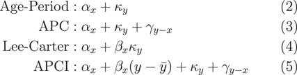
Figure 2 Related models
The first one is the very simple age–period model, which says that the mortality experience in any given year is simply an age component plus a calendar year period component. There is the age–period–cohort (APC) model, an extension which says that the mortality in a given year is a combination of a pure age effect, a pure period effect, plus some so-called cohort effect, which is related to the year of birth.
Third, we have the Lee–Carter model, probably far and away the best known of all the stochastic models in the literature dating back a quarter of a century now, to 1992. That says that the mortality in any given year is a pure age effect plus an age-modulated period effect, the period effect being the κ y and the β x term being the age modulation which allows for the period effect to either be larger or smaller, depending on what year the lives are in that particular year of observation.
Last of all we have the APCI model, the APCI model, which looks, in many ways, quite similar to the three preceding models.
The very simple age–period model is not a model that would be used, in practice, for insurance work. It is far too simple, far too simplistic and does not come anywhere near close to capturing some of the realities of the mortality dynamics. But we have included it here because it is an ancestor model of some of the other models.
Very specifically, if we took the age–period model and just added a so called cohort term, a γ, we would have the rather well-known APC model.
Alternatively, if we took the age and period effect and modulated the period effect by some age-related term, β, we would have the very well-known Lee–Carter model. How does the APCI model fit into this?
The APC and the Lee–Carter models are generalisations of the age–period model, but the APCI model is not in itself a generalisation of these, but it is related. So, for example, if we started with the APC model, we could add a β term, an age-related modulation, and we could change the nature of what κ represents and we would get the APCI model.
This change in the nature of κ is quite important. You will see later how, although the terminology looks the same, with both having a κ and a γ term, the two models are very different and the nature of κ and γ are very different indeed. That is not necessarily obvious just from looking at the formulae; the APCI model is not a straightforward generalisation.
Alternatively, if we took the rather famous Lee–Carter model, add the cohort term and change the nature of κ, we could get to the APCI model.
It is not a generalisation of these models but there are some clear parallels and some possible relation between models. Figure 3 summarises the model relationships.
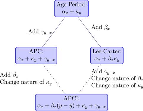
Figure 3 Model relationships
Superficially, we could look at the APCI model as being either an APC model with some Lee–Carter-like β term that had been added or, could think of it as a Lee–Carter model with an added cohort effect plus some other wrinkles.
But, in fact, that is too superficial. There are some very important differences about the APCI model. First, in the Lee–Carter model, the change in mortality, the period-related response to mortality, is age modulated through this β term. That is not the case for the APCI model. The κ term applies without any kind of age modulation term at all. We will see later that that has quite a big impact for insurers.
Similarly, in the APCI model, it is only the expected change, this linear expected change, that is age-dependent because the κ term is not modulated. So it is similar, but not that similar.
In particular, if we were to look at the APC model, the nature of κ, its behaviour, how it looks, what it does, what it represents, is quite different between the APC model and the APCI model. That is something that is not obvious from the maths. The names would lead you to conclude that the APCI model is a generalisation of the APC model. But, as we will see shortly, it has a very different behaviour from the other two models. Although it is related, it is not a generalisation of either.
I will talk a little about the fitting and constraints of these models. All of these models have a potentially infinite number of parameterisations. Take the age–period model as a very simple example. We remember that the age–period model just had two terms (age effect and period effect).
What we could do is define a new age–period model α prime and we could add a constant υ to each one of the α x terms. We could deduct the same constant υ from all the κ terms. When we add α prime and κ prime together: we have exactly the same fit.
There is an infinite number of possible values of υ here. There is an infinite number of possible parameterisations for the age–period model. The same applies to the Lee–Carter and the other models. They have, potentially, an infinite number of parameterisations. To fix on a particular parameterisation, you need to impose what we call an identifiability constraint.
We will have to select these constraints to impose some kind of desired behaviour as part of the fit.
A crucial aspect is that these identifiability constraints will not change the fitted value of the force of mortality at any age or year. So the fit is invariant, but the parameters are obviously different.
The choice that you, as an analyst, make for identifiability constraints is driven by what sort of interpretation you want to place on the parameters, and how you might want to go about forecasting them. This is a choice that the analyst makes but it will not change the fit of the model.
We go back to the age–period model as an example. If we imposed a constraint that the sum of the κ values should be 0, this will not change the model fit but it will mean that the α parameters are very broadly the average of the log of the force of mortality at each age across all the periods.
It does not change the fit, but by imposing this identifiability constraint, it will make the α parameters have a particular and useful interpretation that α x is just the log of the force of mortality at age x, or the average of the log of the force of mortality.
As for our other models, for the age–period model we only need one identifiability constraint and that will nail down all the parameters uniquely. For the Lee–Carter model we need two identifiability constraints. There is a choice and quite a number of different constraint systems. You could use the Lee–Carter model. The commonest is Lee and Carter’s original one. As with the age–period model, we have forced the sum of the κ to be 0 to give this interpretation of α x . Additionally, Lee and Carter suggested forcing some of the β values to be 1.
For the APC model, again we forced the sum of the κ terms to be 0 which gives us a handy interpretation of the α x terms.
Additionally, we forced the sum of the cohort terms to be 0 and we also forced the linear adjusted or linear weighted sum of the cohort terms to be 0.
This very last constraint comes from Cairns et al. (2009), where they wanted the cohort terms to not only have a mean of 0, but also not have any linear trends for forecasting.
The APCI model needs more constraints than this, as we see in Figure 4.
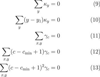
Figure 4 Identifiability constraints for the age–period–cohort improvement (APCI) model
In fact, it needs five. Again, we have the sum of the κ terms being 0 and we have this interpretation of α x . Then we have some additional terms. We have different constraints.
We have, again, the sum of the cohort terms should be 0. We also have this constraint that there should be no linear trends and that there should be no quadratic shape to the γ terms.
It is worth noting that this is one of a number of subtle but important differences between how we fitted the APCI model and how the CMI did it. In the CMI’s working paper, they enforced that the sum of the cohort terms should just be 0. But that has a drawback that a cohort with only one observation has the same weight in the calculation as a cohort with 30 observations. That does not strike us as being particularly good because obviously the cohorts at the edges with few observations have far greater uncertainty.
What we do is we follow the proposal from Cairns et al. (2009). That is a very well-known paper in the North American Actuarial Journal. What they said was that the sum of the cohort terms should weight according to the number of times the cohort term appears in the data. So if a cohort has 30 observations, it has a weight value of 30. If a cohort term only has five observations, it only gets a weighting of five. This way, the cohorts at the edges with a few observations get correspondingly less weight in the calculations.
We think that this is a preferable approach to dealing with cohort terms, so we have adopted this approach. There are more details on this approach and weighting cohorts at the back of the paper in Appendix C.
Looking at the APC and the APCI models, they are all linear. They all use identifiability constraints, or they will need identifiability constraints if you want to nail down a particular parameterisation. They all, potentially, have parameters that can be smoothed.
What we do in our models, similarly to the CMI, is we assume that in the two-dimensional grid we have death and exposure for each age in each calendar year. We assume that the number of deaths observed has a Poisson distribution with a mean which is just the product of the exposure, mid-year exposure, and the force of mortality, mid-year.
We can fit the age–period, APC and APCI models as penalised smooth generalised linear models (GLMs). These are linear models so they can be fitted as GLMs.
As Iain (Currie) covered in one of his earlier papers, we can also fit the Lee–Carter model as a GLM but you have to do it as a pair-wise step conditional on one of the parameter sets.
This is another important difference between how we fitted our models and the CMI fitted theirs. Iain published a paper in the Scandinavian Actuarial Journal in 2013 which, I think, is far more significant than has yet been realised. At the core of the generalised linear model, there is what is called the iterative re-weighted least squares algorithm, which is a very powerful means of quickly fitting a generalised linear model in such a way that it allows for quite a wide variety of distributions, but also for a wide variety of link functions.
What Iain did in his 2013 paper was something very impressive indeed. He has extended the GLM-fitting algorithm so that it will not only maximise the likelihood, as it does with the original Nelder and Wedderburn algorithm, but he has extended the algorithm so that it will also simultaneously maximise the likelihood while also applying your choice of any linear identifiability constraints that you may wish to apply, while also smoothing the parameters that you have chosen to smooth. You get everything in one: model fit, constraints will be applied and the parameters you want to be smoothed will all be smoothed all in one. It is what you might call an integrated process.
This is in contrast to the CMI’s approach where the maximisation of the likelihood, or penalised likelihood, is one stage and there is a separate smoothing stage added on and then there is a separate constraint application stage.
One of the incredible things about Iain’s algorithm is that it does all these things in one integrated algorithm. It is relatively straightforward to implement in programming terms. I strongly commend this to you and details are in his 2013 paper. It is a very, very powerful tool to use. It is a major development and it will have a lot more application in future.
One point to note is that identifiability constraints do not always have to be linear. For example, in the Lee–Carter model, both Girosi and King and Iain and I presented non-linear identifiability constraints. Cairns et al. used some non-linear identifiability constraints as well. However, proving that an identifiability constraint is a constraint is a lot harder if it is not linear. It is a lot easier if it is a linear constraint. The Currie algorithm will only work with linear constraints. That is not too much of a constraint.
Moving on to parameter estimates, we fit our models, the age–period, the APC and APCI models as either straightforward linear models, generalised linear models or the Lee–Carter model with the conditional two steps. You can see what we get for the α x estimates for the four models in Figure 5.
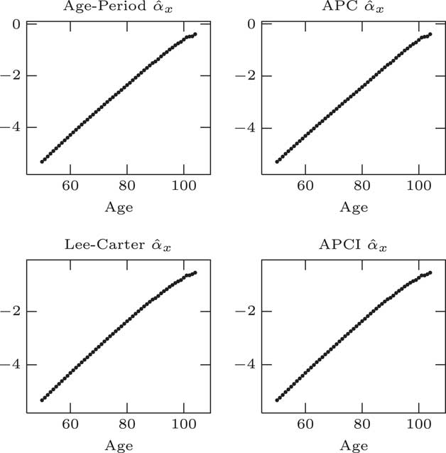
Figure 5 α parameter estimates
Unsurprisingly, they look almost identical. That is because they are basically doing the same job in each case. α x is, essentially, approximately the log of the average log mortality at a given age across the entire period. α x plays the same role, average log mortality by age, as long as we apply this identifiability constraint that the sum of the κ values should be 0.
It is worth noting that although we have used a single parameter for every single age, that is far more parameters than we strictly need. That is clearly an over parameterised part of all the models. These 50+ parameters, are, strictly speaking, unnecessary. There is a very clear smooth pattern. These 50+ parameters could be replaced by a much simpler smoother curve.
What we could do is to reduce what is called the effective dimension of the model by replacing these independent α x parameters with some kind of smooth curve. It would not change the model in any material way.
The β parameters for the Lee–Carter model and the APCI models: at first glance they look quite different; but in fact if you plot minus for the APCI model, you can see in Figure 6 that the β parameters in the Lee–Carter and the APCI models are doing strongly similar jobs – age modulation of the period effect in the case of Lee–Carter model or the linear trend in the APCI model.
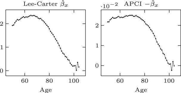
Figure 6 β parameter estimates
Looking at that, it is a more complex shape than it is for α x . It is still an over-parameterisation. We do not need all of these β parameters. We could replace them with a smooth curve and not make any material change to the model.
β x plays an analogous role in both the Lee–Carter and APCI models, although the β x in the APCI model operates only on a linear trend term. We would note that we think to make the β term in APCI models more directly comparable with Lee–Carter β it would have been better multiplied by y bar minus y rather than y minus y bar. We have stuck with the parameterisation that the CMI used.
Like α, the β x could be usefully replaced with some kind of smooth curve to reduce the effective dimension of the model. One important aspect is that smoothing the β x improved the forecasting behaviour of the model.
A paper from Delwarde, Denuit and Eilers shows that smoothing the β x terms in the Lee–Carter model helps reduce the risk that projections at adjacent ages crossed over in the future. So the smoothed β x not just reduces the dimensions of the model, but it is important to smooth its improved forecasting properties as well.
We note, as an aside, that the APCI model has two time-varying components. It has the age-dependent linear trend, which is modulated by β x , and also has an unmodulated period effect, κ y .
The α x and β x terms seem to play very similar roles across the models, where they are present, but what about κ y and the cohort terms?
We can see in Figure 7 that for the age–period, APC and Lee–Carter models, κ plays a very similar role. Not quite the same values but certainly the same behaviour, the same pattern, the same trend and maybe the same methods used for forecasting in these three cases.

Figure 7 κ parameter estimates
We can see here that κ in the APCI model has a very different nature, a very different behaviour, a much less obvious trend and is much harder to forecast as a result.
We can say that while α and β play very similar roles across all models, κ y only plays a similar role for the first three models; it plays a very different role in the APCI model.
Partly as a result of this, the κ values and the APCI model have much less of any kind of clear trend or pattern when it came to forecasting. As we will see, the κ values in the APCI model are very heavily influenced by other structural choices that you make when fitting the APCI model.
If we turn our attention to the cohort term, γ y−x , we can see in Figure 8 that there are very different patterns under the traditional APC model and the APCI model – radically different patterns are coming out here. This is in part because of the different constraints that are applied. The APCI model has an additional constraint, quadratic constraints, which the APC model does not have. This has radically changed the structure and the shape of these γ terms.
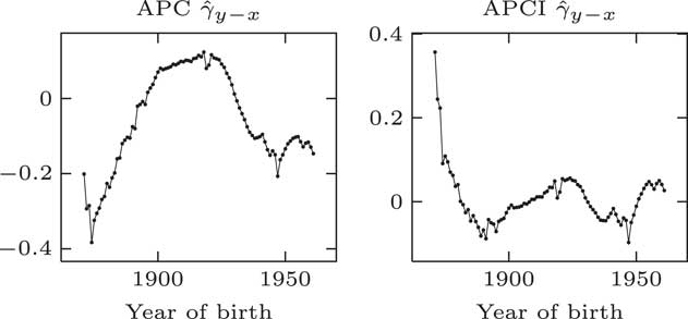
Figure 8 γ parameter estimates
This leads to an interesting question. The γ terms appear to play directly analogous roles in the two models. They look as if they are cohort terms or represent cohort effects. The values taken in the two models are very different and the shapes displayed are very different. If you take a given year of birth, the two models have very different ideas of what the γ term is.
If the shapes of these γ terms and the values are so different between the two models, what do they represent? Can they represent a cohort effect at all if two different models have a very different idea of what the so-called cohort effect should be?
It turns out that the γ terms, although they look like cohort effects, do not have an interpretation which is independent of the model. As Iain said, they do not have a life of their own. They only have a life – an interpretation – with respect to the structure of the model within which they are fitted, and with respect to the other parameters and the constraints. The γ terms are not independent cohort effects or any kind of independent estimate of a so-called cohort effect.
In conclusion here, we do not think that the γ terms describe cohort effects outside of the models; we do not think that they represent the cohort effects in any meaningful way.
With regards to smoothing, the CMI, when they presented the APCI model, smoothed all the parameters, the α, β, κ and the γ. But, as we have seen, only the α and the β terms exhibit sufficient regular behaviour that means they can be smoothed without making any material impact on the model. We ask the question: does it make sense to smooth the κ terms or the γ terms in the APCI model? We do not think it makes sense to smooth either of them because they do not exhibit smooth, regular behaviour.
In the CMI model, there is a smoothing parameter for κ called Sκ. There are corresponding S values for α, β and γ. When maximising the likelihood, it is the CMI maximising the penalised likelihood in the same way as we do here, and it has the smoothing penalty for κ based on the second differences. It multiplies this by the 10 to the power Sκ. It is applying fairly heavy smoothing for κ.
The value for Sκ is set subjectively. The CMI state in their working paper that it is up to the analyst to decide what value to pick for Sκ. They present the results taking a couple of different values.
What is the impact of smoothing κ if so far as we are concerned it ought not to be smooth? To quote from the CMI working paper: life expectancies produced by the APCI model are rather sensitive to the choice that is makes for the Sκ term, with the impact varying quite widely across the age range, with a particularly large impact at ages above 45.
Sκ has a large impact in part because, as we saw earlier, the κ terms do not have any particularly strong pattern. They do not have any particularly obvious trends that one could extrapolate or forecast. In fact, the κ term in the APCI model is really like a leftover collection of other aspects of the model. That is why the values are relatively small. That is why they do not show any particularly clear behaviour.
I do not want to call it a residual because a residual has a clear meaning in statistics. If κ is like the leftover of other aspects of the model, and it is not applied with any kind of age modulation, should you be smoothing it at all? If you smooth something that is essentially a leftover that is very sensitive to other structural choices made in the model, then you are going to obtain some quite radical changes in direction if you try to forecast this smoothed entity. This is one reason why the life expectancies in the CMI’s working paper proved to be so sensitive to the choice of Sκ smoothing parameter
We turn our attention now to some value at risk considerations. One of the interesting things about longevity trend risk is it obviously unfolds over several decades over the remaining lifetime of your annuitant. It is a requirement of our regulations that we should look at all risks, including longevity trend risk, through this 1-year value at risk style prism.
What we did with the APCI model, and others, is we took the approach that we set out in our paper of 2014, where we take a model, we use it to simulate the following year’s mortality experience; we add this experience to the data; refit the model and then look at the forecast that comes out of it; value the liabilities under this forecast; and then repeat 1,000 times, 5,000 or, however, many times you want.
This will give us a density, a distribution if you like, of the liabilities under the 1-year value at risk assessment.
You can see in Figure 9 an example from the 2014 paper. This is from a Lee–Carter model. This gives you an idea of the different forecast mortality rates at age 70 that come out of this value at risk process just from simulating and refitting the model. You can see the different forecasts and it will obviously result in different reserve values.
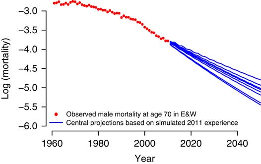
Figure 9 Sensitivity of forecast
For the APCI model, for parameter uncertainty, we use an Autoregressive Integrated Moving Average (ARIMA) model without a mean for all the γ terms. We use ARIMA models with means for κ terms under the age–period, APC and Lee–Carter models. We saw earlier that the κ process has a clear trend, a clear pattern. We are using an ARIMA model without a mean for κ in the APCI model.
You can see in Figure 10 that each of the different models has quite different looking densities. We can see some of the models are broadly unimodal, the age–period and the Lee–Carter models are unimodal; but the APC and the APCI models are bimodals.
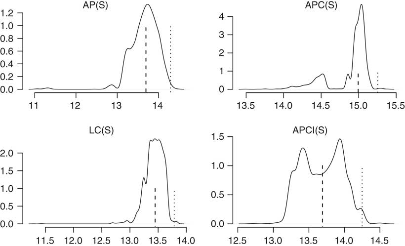
Figure 10 Liability densities
This follows through into some of the conclusions you can draw from the value at risk assessment. The APCI model is particularly interesting. It is almost symmetric, bimodal and symmetric, where the median or the mean is not anywhere near likely to be one of the most commonly occurring values. The value at risk, the 99.5 percentile, is quite far from the mean. It is not the case for some of the other models there. There is a very, very different picture for the value at risk densities in the four different models.
We also did similar calculations for some other models in the paper, but we will not cover those at the moment.
We have a variety of density shapes, not all are unimodal. It is possible, even just using a Lee–Carter model which is unimodal, for some data sets to get bimodal distributions under the value at risk calculations. This is by no means a feature that is restricted to the APC and APCI models. These value at risk calculations are not always unimodal.
For me, the very different pictures of these densities emphasise just how much variability there can be between different models, even ones that seem to be closely related. And for me, this emphasises the over-riding need to use several different models when you are looking at setting not just your best estimate but also when you are setting your capital values under a value at risk approach.
What we have in Figure 11 is the value at risk percentages for a variety of ages for the four models.
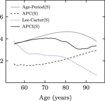
Figure 11 Value at risk
You can see the four different models, despite having relationships between them, paint very different pictures as to what the value at risk capital should be at each age. For me, this is just a reminder why it is important to look at the outputs from many models when you are exercising your expert judgement.
One question which cropped up was why do the capital requirements reduce with age for the Lee–Carter model but not for the APCI model. The answer is that this κ term for the Lee–Carter model is modulated by β x , and β x tends to be small and close to 0 under the Lee–Carter model for high ages. In the APCI model, it is entirely unmodulated and this leads to comparatively larger impact at the older ages. That is one reason why the APCI model paints such a different picture of the capital requirements.
In conclusion, we think that the APCI model is implementable as a fully stochastic model, not just for deterministic purposes. We can see that the APCI model shares a number of features, and also drawbacks, with the age–period, APC and Lee–Carter models.
We have seen here that smoothing the α and β terms of the APCI model is sensible. It does not distort the model. Indeed, smoothing β will improve some of the forecasting properties. We do not think that it is sensible to smooth either κ or γ in the APCI model. They are not well behaved, regular processes. Smoothing them will lead to distortions.
Another recommendation is that the Currie algorithm should be sought out and implemented. It is particularly useful for fitting these penalised, smoothed GLMs.
The Chairman: Thank you for that presentation. I should now like to open the discussion to the floor.
Mr T. J. Gordon, F.I.A.: I am speaking on behalf of the mortality projections committee of the CMI, of which I am the chair. We are strongly in favour of debate that enhances general understanding of mortality modelling and, in particular, throws light on tools as CMI users. We welcome the paper.
We do, however, have some specific points to make. First, the APCI model is used by the current CMI projections model, but it is important for readers of the paper who may link the conclusions of the paper to the validity of the model, to understand that the CMI does not use the APCI model as a stochastic model. The APCI model is used solely to obtain initial improvement rates for projection split between age–period and cohort-related improvements.
The CMI model uses a different model from APCI to project future improvements. In both cases, we view the models as frameworks to help us to arrive at projections and not as the drivers of the projections.
I also have some observations on the paper itself. First, comparing κ terms between the APCI model and the other models considered as is done implicitly in Figure 7 above, is potentially misleading. The other models have κ representing all period dependency, whereas the APCI model is represented by the κ term plus the β term times time.
It would have been more informative to have plotted this, I think.
Second, the paper’s conclusion states that the κ term in the APCI model, which captures period variation over the average trend, does not look like a suitable candidate for smoothing. There is a danger that readers of the paper may therefore conclude that the CMI model is doing something wrong by smoothing the κ term.
I should like to point out that in the CMI model we are specifically looking through to the underlying trend after discarding both the idiosyncratic and the systematic annual noise. The smoothing approach used in the CMI model is mathematically identical to modelling the κ term as an ARIMA(0,2,0) process; that is to say, it treats mortality improvements as a random walk which, given the menagerie of ARIMA models on display in Appendix E, is, prima facie, reasonable in our view and certainly fit for the purpose of deriving the initial improvement rates.
Further, it allows users to select the underlying variability of that random walk. κ is a deliberate feature of the model that allows you just to take a view on how much weight to place on recent changes in mortality improvements.
Finally, the quadratic pattern of cohort dependence on year in the graphs of γ and Figures 5 and 7 in the paper for the constrained and unconstrained APC model, and in Figure 8 in the paper for the unconstrained, although not the constrained, APCI model, we think should be a red light for the authors.
We strongly suspect this feature is an artefact of how the models have been fitted. I refer to Jon Palin’s paper: “When is a cohort not a cohort?” presented at the 2016 international longevity mortality symposium.
This could easily be addressed by different constraints and/or priors.
I conclude my remarks by saying thank you to the authors for an interesting and thought-provoking paper; and again stressing that the CMI welcomes debate. The more scrutiny of components of the CMI model, the more robust the model is likely to be. Thank you.
The Chairman: There are plenty of points there. Were there any points that you would particularly like the authors to respond to right now?
Mr Gordon: I guess there are two particular points. One is the equation you put up for smoothing the κ terms in the CMI model is mathematically the same as having a random walk mortality improvements. When you go on to fit ARIMA processes to the κ term in the other models, the CMI model is implicitly already doing that in the calibration of the APCI model. Those smooth κ terms are no different from the ARIMA process terms that you get for your κ series. They are the same animal, in effect.
Calling one smoothing and another an ARIMA process is drawing an artificial distinction. The CMI model is not designed to be projected as a stochastic model. In other words, in our view, it is fit for purpose because we are trying to understand the underlying smoothed process.
The second point is similar. We think that the quadratic pattern, the parabolic pattern, to those cohort terms that you get from the other models does not pass muster from a common-sense point of view.
Those are the two points. One is: what you have called smoothing is nothing other than ARIMA(0,2,0). Mathematically, it is the same, fitted by maximum likelihood with a prior. The second is that we think that the cohort pattern in the other models is unrealistic.
When you draw the graph of the constrained APCI model and note that there are probably better ways of achieving that, we do not think the fact that it is constrained and has an overall flat cohort pattern is a bad thing. We think that is a good thing.
Dr Richards: I can pick up the last point. It, as you say, does not make too much of a difference which constraint system you choose. I agree the purpose of the selection of which constraint system you want to use is to impose the behaviour that you want on a particular set of parameters.
In the case of the APCI model you have three constraints on the γ terms, one of which is, as you alluded, to remove the quadratic type behaviour or particular shape.
It is perfectly valid to do this if, for example, you wanted to forecast the γ terms for the unobserved cohorts. I do not have any problem with that.
I am not sure I follow the points about the κ process being an implied ARIMA(0,2,0) process. That is presumably one without a mean.
Mr Gordon: Yes.
Dr Richards: I am not entirely convinced that they are completely identical. I will take your comments away and study them.
The Chairman: Would anybody else like to comment or ask a question?
Professor A. D. Wilkie, F.F.A., F.I.A.: I have done a fair bit of time series modelling in a different field. I do not quite understand Tim Gordon’s point that a deterministic smoothing can be the same, or is the same, as an ARIMA model. It may be in some circumstances.
If you say the ARIMA model is just a random process, each year is independent, with some distribution, then if you put a straight line through the middle of it and say that they are all equal to the mean, then you have the same smoothing.
If you think of an Autoregressive 1 (AR1) model, with quite a high standard deviation, then it jiggles up and down around the mean but it will go quite a long way up from the mean and then back down again and below the mean and back up again. Just substituting the mean all the way through does not the same forecast for the future, because the future forecasts for an AR1 model depend on where you are in your final year. It does not just depend on the average. You would go gently. The forecast would move exponentially down towards the mean.
Those are the two simplest models. I do not quite see how they can be the same.
I was going to make a quite separate point, and this is a very general point about stochastic modelling. I think you have a fair amount of allowance for uncertainty in the parameters. Is that right?
Dr Richards: Yes. There is an allowance for parameter risk; but for the value at risk calculations the real driver, the majority driver, of the uncertainty comes from the 1-year uncertainty.
Prof Wilkie: Yes, it would do. When you have done the smoothing – for the α term, you fit a Gompertz straight line, pretty well. But what is the slope of that? You are not sure of what it is. You are pretty sure. There is very small error in it. But there is some uncertainty about that.
With the time series modelling, there is some uncertainty about all the parameters you are getting in.
I am doing some work on a quite different field of investments. I am introducing what I would call a hyper model, a new term, where at the beginning of each simulation, one simulates the parameters for that simulation from some distribution of the parameters, which I suppose is what you are doing as well. Then you simulate using the innovations that you are expecting to come in the time series modelling according to the standard deviation you fitted. But not the standard deviation you fitted overall, rather the standard deviation for that particular simulation.
That means you have twice as many, plus a covariance matrix of, parameters, but you are allowing, I think more reasonably, for the uncertainty in your modelling because all your estimation is done over some finite time period. It is not much more than about 40 years, the time series modelling. It is pretty small. So the standard errors of the parameter estimates are reasonably large.
I think that this is a good policy to use for any actuarial simulation in any field you like.
But a feature about it is that when you are normally doing this sort of fixed parameter fitting, you are wanting a parsimonious model with as few parameters as you can get away with. If one of the extra parameters in the time series model, or in other models, marginally might not be significant, you then miss it out.
If you are wanting to allow, from an actuarial point of view, for the reasonable amount of uncertainty, you should possibly leave it in and be more generous rather than parsimonious.
From the point of view of value at risk, the finance director wants the lowest value you can find. If you presented him with ten models, he will choose the lowest, I suppose. But the prudent actuary should more or less be choosing the highest that you can find because that is the one where there is the most reasonable uncertainty.
I have not done enough of this to know how to balance what is a reasonable extra to put in or a skimped extra to put in. I have been fitting, in one context, straight distributions and skewed distributions with the same sort of parameter structure. Rather than putting skewed coefficients as 0, and saying that it is fixed, it might be a bit different. I am inclined to say it might be different in the future for the investment models that I am looking at, so I will allow for the uncertainty of my skewness estimate even though it is pretty close to 0.
I do not know whether that is a general point that would be useful to make or whether the authors have any feeling about it. It is on a totally general point about the actuarial modelling.
The Chairman: If you are a life office practitioner or a pensions consultant who analyses longevity and uses stochastic models as part of that analysis, I would be very interested to hear whether you feel that this is a material and very useful contribution to the array of stochastic models that you might use and how you think you might use it in the future, particularly because, being slightly more generalist, we do not fully understand all of the statistical nuances of all the models, but we try to use them as best we can to manage longevity risk.
Any thoughts on whether this APCI model will go into the pantheon of models that will be used by life offices and pensions consultants analysing longevity?
Dr I. D. Currie: If I could just come back to what Tim (Gordon) was talking about, one of the big problems in these kinds of models is the interpretation of parameters. I think it is very easy to be misled.
If you take the age–period model, a simple model, you put a constraint on the time term, and lo and behold, it is quite obvious that the α terms correspond to overall mortality and the κ terms refer to the general trend in mortality over time. One is perhaps encouraged to think this will always be the case, whatever kind of model you have.
If you then move to the APC model, what you are certainly doing here is modelling the strength of the cohort influence on mortality. What you are definitely not doing is being able to identify the individual γ with particular cohort effects.
One is a bit misled by the success of this interpretation in the age–period model into thinking that it might extend further down the line. In the APC model it is definitely the case that the constraint has a huge influence on the kind of values that you will obtain.
It is not obvious what the constraint system should be. Very different values can result. Beware of over interpretation of that γ term.
The Chairman: I have come across a number of circumstances where a model seems to fit the data very, very well but does not necessarily produce plausible projections. I do not see why there should not be a sweet spot where there is a model which does both. Yet, it seems to be quite elusive. I am assuming that there is not a trade-off between fitting the data very well, or parsimoniously, and producing good projections. It is just that it is very hard to find.
Dr Richards: It is certainly the case that goodness of fit to the data should not be the sole criterion for judging the quality of our projection model. This, in part, came through from the Cairns et al. (2009) paper, where it compared eight different models. The Renshaw–Haberman model is an example. It fitted the data a lot better than the Lee–Carter model. But it does not have particularly good behaviour in terms of forecasting.
There is not an obvious, direct trade-off between goodness of fit and forecasting. You can have good fitting models that do not have good forecasting behaviours. You can have models, like the Lee–Carter one, that do not fit the data as well but have quite good, robust behaviours.
The Chairman: And having an objective criterion like the Akaike Information Criterion (AIC) and the Bayesian Information Criterion (BIC) does not resolve all of that issue?
Dr Richards: It does not, no. In fact, Torsten and my paper from last year comes back directly to David Wilkie’s point about your choice in the ARIMA model. We showed, just within the particular data set, within a particular fitting of the Lee–Carter model, there is a variety of different ARIMA models to be fitted.
The best fitting model for male data in England and Wales happens to have some additional parameter risk compared to other models because the model is borderline non-stationary – just within the bounds of being stationary.
Although it was clearly the best fitting model, in terms of the AIC, and the next closest models were not sufficiently close that you would choose them, it had instabilities that these not quite so good fitted models did not have. It is a very difficult issue to manage. You can often find good fitting models having unwelcome properties for forecasting.
The Chairman: Which is presumably why you talk a lot about model risk.
Dr Richards: Which is why we talk a lot about model risk, yes. It is absolutely essential to use lots of different models and not just variations on a particular flavour; models that belong to completely different families.
Prof Wilkie: I should have said in the very first place, I was very impressed with how mortality forecasting has gone since I was involved with it about 30 years ago. The CMI was extremely crude. This is marvellous.
As regards the last point, I am going to jump to a different example. If I take the yields on index-linked bonds for the period that they have been issued, the best fitting AR1 model is one with a parameter bigger than one.
They started at 2% and then went up to about 3.5%. They have gone down and down and become negative. My first model that was tracking log yields does not work. You have to go on to just straight yields without the negatives.
If you had the best fitting model then, in the long run, the yields on index linked bonds become more and more negative until in 100 years’ time you are −1,000% or something. That is just nonsense.
You have to put certain constraints on the model if the long-term behaviour is not sensible.
A similar, but quite a different, thing, occurs in an old actuarial textbook about population forecasts made for England and Wales in the 1930s. At that time, the birth rate had been declining. It was assumed, in one of the projections (artificial), that the birth rate would decline linearly, until, about 1950, it reached 0 and there would be no further births in Britain at all after that date.
They did not say this is so much rubbish. What we should be doing, even if it is going down, is taking it down not linearly but exponentially. The whole concept of a linear reduction in mortality is nonsense because after some future year everybody becomes immortal. That is just implausible.
There is no point in fitting a totally unreasonable model, even if it fits nicely the data you have. Particularly with ARIMA models, or any long-term projection model, you have to think about what the long-term structure of the model would be.
Things can appear to go wrong. You may have in the period from, say, 1930 to 1980 inflation which was pretty steadily increasing. One of your best forecasts might have been for it to go on increasing forever.
Similarly with mortality. If you have a period of increasing mortality (I think in Russia after 1990), you might make the mistake of forecasting it going up again forever instead of saying that this is an unfortunate blip and it will come back down again and we will find a way of at least stabilising or possibly reducing.
That is just a general point. You have to use what are long-term, sensible models and not the best fitting ones. And then fit the sensible ones as well as you can.
Dr T. Kleinow: I should like to make a few comments on that subject. I completely agree of course. You want to look at the projection and properties of the models. Also, for exactly the reason that you just mentioned, that you might get unrealistic projections, we think that including a stochastic turn in the projections is so important and also, as you mentioned earlier, to look at the parameter risk in the estimated improvement rates or in the time series parameters, or whatever those parameters might be.
We did that and we looked very carefully at the risk that comes from the uncertainty about the parameters which we have from past observations, we estimate those from past observations, and compare those to the uncertainty that we have about future improvements and unexpected improvements in mortality.
We found that there is a balance between those two. In the short-term there is the future unexpected improvements which are more important but in the long-term it is exactly the parameter uncertainty that becomes so important. That is absolutely right.
Looking at stochastic models, and looking at parameter uncertainty, it takes some of the problem away of getting very unrealistic projections because we do not have just one projection, we have many. We have many scenarios. We have probabilities that we can put on those scenarios.
The Chairman: Just a quick point related to what you said about the plausibility of the model, you justified not smoothing the κ terms, partly in response to the way that the un-smoothed κ looked when you plotted them.
Is there a case for saying that, even if they do not look particularly smooth when you calculate them, it is logical that the κ terms would be smoothed in some way? That is the way that mortality works and therefore you impose a little bit of structure on the κ just from that point of view, rather than just staring at the κ terms that come out of the model.
Dr Richards: I think that argument can apply to the α and β terms. It is not clear to me that that would apply to the κ terms precisely because they pick up period effects which I do not think they should. There is no underlying rationale as to why they should be smooth, in the same way that you can understand why the α x should be smooth because the mortality of a 50-year old would be higher than a 45-year old, and so on.
Similarly, with the β x . You can imagine the rate of improvements can be different, or higher, at age 60 and 70 but once you get to age 100 the improvement will be lower.
You can understand fairly simply why there would be fairly smooth progression, potentially, from one age to the next, and why you would therefore smooth α and β.
I cannot think of a rationale why the κ terms in the APCI model should be an underlying smoothed process.
Dr Kleinow: I completely agree with that statement in particular because in the APCI model there is already a very smooth period term which is β (xy), so already there is a linear improvement in mortality built-in by taking β (xy) and estimating the β x .
Then on top of that, you have the term which captures unexpected improvements. To smooth those seems to be wrong to me. The very nature of mortality is that it cannot be projected with certainty. In the APCI model I would say the κ y is the one term that takes the model stochastic, and that allows for different scenarios to unfold in the future.
Therefore, I would not smooth those parameters.
Prof Wilkie: I will come back on that one. Obviously, mortality should be fairly smooth by age, as Stephen (Richards) says. There can quite well be unexpected upwards movements in mortality. It is very easy for a lot of people to die from infection or catastrophe. It is rather harder for unexpected downward movements to occur.
But take 1919 and the “flu epidemic”, or any of the years a bit before your period, when there were quite severe “flu epidemics” in Britain, or in some years when there have been extremely hot summers and so certain countries south of here have had rather high mortality, you can expect the mortality rate from year to year to jiggle up and down a lot. That is fairly normal.
The slow, gradual medical improvement, you may say, goes reasonably smoothly, yet if you go back to some old CMI figures there was a remarkable drop in mortality in the civilian population in Britain in 1942. After 1942 almost no age reached as high as the 1941 figures. The same thing is not in population figures; it is in the assured lives. Why it is there, I am not quite sure. It is a little bit too early for penicillin. But something like penicillin can produce a step change downwards. Something like a tsunami in some places can produce a step change upwards – but only temporarily.
The Chairman: I should like now to invite Gavin (Jones) to close the discussion. Gavin Jones is the global head of Longevity Pricing at Swiss Re. He has worked in longevity risk and its transfer since 2003 and co-authored, with Stephen Richards, the Staple Inn Actuarial Society (SIAS) paper “Financial Aspects of Longevity Risk”.
Mr G. L. Jones, F.I.A. (closing): The CMI model, as it has evolved since the introduction of cohort projections, first and foremost, offers people a transparent means of communication and has enabled market participants to express a point of view. That has been accomplished by effectively having a different process for the historic fit and for the projection which has been deterministic in nature.
I welcome the sessional paper where the Edinburgh-based authors focus on the stochastic implementation of the current historic fit process, and apply that to projections. Given the huge development over the 25 years since the original Lee–Carter model in mortality modelling, particularly over the last decade, that always provides insights, comparisons and challenges.
Any additional model provides one means of summarising a version of understanding and also gaps in that understanding. For example, the material differences that are shown in the paper on the life expectancy between, for example, the APCS and the APCI model, highlighting, as discussed earlier, the prevalence of model risk.
That implementation of a stochastic model provides a distribution of outcomes and associated regulatory capital calculations. As Tim noted, that is not necessarily what the users of the CMI model will apply it for.
The projection process requires an approach to identification of parameters particularly of κ and γ, where the authors challenge the identifiability of a signal within that process.
That is not a statement that the model is intractable, simply that those parameters, with a constraint applied, highlight fundamental problems in the fit and forecast of mortality.
In order to apply the model, some level of explicit choice is required from its users. The published CMI model provides a simple way for participants to engage in discussions around transaction pricing or funding level of pension schemes.
I would also bring to the attention of the audience the recent Society of Actuaries publication on components of historical mortality improvements which includes the CMI model as one of the variety of models used in the United States mortality improvements.
Underlying the application of stochastic models is the view that there is some form of parameterisable driver which is going to evolve with time.
Whether we work in the context of potential step changes in mortality rates or health care provision, it is a reasonable question as to whether that is a good structural description of mortality evolution, and whether a satisfactory calibration can be from a purely mathematical fit or whether we will need input from outside the model.
As a profession, to understand the range of prospective mortality drivers, we can and do look beyond the confines of explicitly modelled risk.
It is notable that recent awards of the Nobel prize for economics have included two individuals, Angus Deaton and Richard Thaler, both of whom have been associated with the analysis of mortality risk, albeit from very different directions.
Their research addresses problems that would have been familiar to Adam Smith. For us, as interest rates have fallen over the last two decades we too have seen mortality in the form of longevity risk return to the centre of the of our own profession, and indeed our shared roots in the Scottish enlightenment. With that, I would thank the authors.
The Chairman: Thank you, Gavin. On behalf of all us, thanks are due to the authors of the paper, to Stephen, for his presentation and to Gavin for closing a discussion and to all those who have participated in this discussion.
Written Contribution: The following contribution was received from the authors in response to Mr Gordon.
We note the point that the CMI does not use the APCI model for projection, merely to use its parameters in calibrating its deterministic targeting spreadsheet (CMI_2016). It is a curious situation: the APCI model is deemed good enough for fitting to past data but not for projecting future experience! We would note, however, that the APCI model cannot be used to split between age-period and cohort-related improvements, not least because of the identifiability problem: the period and cohort terms estimated are a function of the (arbitrary) identifiability constraints selected. If one changes the identifiability constraints, one gets the same overall fit in the same model, but with potentially very different parameter estimates.
We agree that the
 $$\kappa _{y}$$
terms in the APCI model are not comparable with the terms of the same name in the other models. However, we do not consider Figure 4 misleading, as its purpose is to demonstrate this very point. Figure 4 shows the different nature of the similarly-named
$$\kappa _{y}$$
terms in the APCI model are not comparable with the terms of the same name in the other models. However, we do not consider Figure 4 misleading, as its purpose is to demonstrate this very point. Figure 4 shows the different nature of the similarly-named
 $$\kappa _{y}$$
in the four models, and thus the need to consider
$$\kappa _{y}$$
in the four models, and thus the need to consider
 $$\kappa _{y}$$
in the APCI model as a fundamentally different process from
$$\kappa _{y}$$
in the APCI model as a fundamentally different process from
 $$\kappa _{y}$$
in the other three models.
$$\kappa _{y}$$
in the other three models.
Regarding the point about the CMI’s smoothing of
 $$\kappa _{y}$$
being mathematically identical to modelling the
$$\kappa _{y}$$
being mathematically identical to modelling the
 $$\kappa _{y}$$
term as an ARIMA(0,2,0) process, it is worth noting that the CMI’s fitting procedure imposes the ARIMA(0,2,0) structure on
$$\kappa _{y}$$
term as an ARIMA(0,2,0) process, it is worth noting that the CMI’s fitting procedure imposes the ARIMA(0,2,0) structure on
 $$\kappa _{y}$$
and the rest of the model must accommodate this assumption as best it can. The subjectively
$$\kappa _{y}$$
and the rest of the model must accommodate this assumption as best it can. The subjectively
 $$S_{\kappa }$$
chosen
$$\kappa _{y}$$
value controls the variance of this ARIMA(0,2,0) process, and increasing
$$S_{\kappa }$$
chosen
$$\kappa _{y}$$
value controls the variance of this ARIMA(0,2,0) process, and increasing
 $$S_{\kappa }$$
forces
$$S_{\kappa }$$
forces
 $$\kappa _{y} $$
to appear even smoother. This requires that other parameters accommodate the enforced structure to
$$\kappa _{y} $$
to appear even smoother. This requires that other parameters accommodate the enforced structure to
 $$\kappa _{y} $$
, and it removes more of the random year-by-year fluctuations of mortality rates. Removing those fluctuations might give the incorrect impression that improvement rates are smooth over time and can therefore be projected with a high degree of certainty. In contrast, our approach is the reverse of this: we estimate
$$\kappa _{y} $$
, and it removes more of the random year-by-year fluctuations of mortality rates. Removing those fluctuations might give the incorrect impression that improvement rates are smooth over time and can therefore be projected with a high degree of certainty. In contrast, our approach is the reverse of this: we estimate
 $$\kappa _{y}$$
and then see what ARIMA model best describes the resulting process; in Table 9 in Appendix E we find that an ARIMA(1,1,2) model best describes the APCI
$$\kappa _{y}$$
and then see what ARIMA model best describes the resulting process; in Table 9 in Appendix E we find that an ARIMA(1,1,2) model best describes the APCI
 $$\kappa _{y}$$
for UK males, not ARIMA(0,2,0).
$$\kappa _{y}$$
for UK males, not ARIMA(0,2,0).
It is correct to say that an ARIMA(0,2,0) model for
 $$\kappa _{y}$$
in the APCI model treats mortality improvements as a random walk. A mortality improvement is defined as
$$\kappa _{y}$$
in the APCI model treats mortality improvements as a random walk. A mortality improvement is defined as
 $$1{\minus}{{\mu _{{x,y}} } \over {\mu _{{x,y{\minus}1}} }}$$
, i.e. it is the relative change of the mortality rate in time while holding the age constant. Under the APCI model, the mortality improvement at age
$$1{\minus}{{\mu _{{x,y}} } \over {\mu _{{x,y{\minus}1}} }}$$
, i.e. it is the relative change of the mortality rate in time while holding the age constant. Under the APCI model, the mortality improvement at age
 $$x$$
in year
$$x$$
in year
 $$y$$
is therefore:
$$y$$
is therefore:
 $$\eqalign{ {1{\minus}{{\mu _{{x,y}} } \over {\mu _{{x,y{\minus}1}} }}} \hfill & {{\equals}1{\minus}{{\exp \left( {\alpha _{x} {\plus}\beta _{x} (y{\minus}\bar{y}){\plus}\kappa _{y} {\plus}\gamma _{{y{\minus}x}} } \right)} \over {\exp \left( {\alpha _{x} {\plus}\beta _{x} (y{\minus}1{\minus}\bar{y}){\plus}\kappa _{{y{\minus}1}} {\plus}\gamma _{{y{\minus}1{\minus}x}} } \right)}}} \hfill \cr {} \hfill & {{\equals}1{\minus}\exp \left( {\beta _{x} {\plus}\kappa _{y} {\minus}\kappa _{{y{\minus}1}} {\plus}\gamma _{{y{\minus}x}} {\minus}\gamma _{{y{\minus}1{\minus}x}} } \right)} \hfill \cr {} \hfill & {\,\approx\,{\minus}\beta _{x} {\minus}(\kappa _{y} {\minus}\kappa _{{y{\minus}1}} ){\minus}(\gamma _{{y{\minus}x}} {\minus}\gamma _{{y{\minus}1{\minus}x}} )} \hfill} $$
Equation (1) shows that mortality improvements under the APCI model comprise three components:
∙ A
 $$\beta _{x}$$
term, which is age-dependent but estimated from the data and presumed constant in the forecast.
$$\beta _{x}$$
term, which is age-dependent but estimated from the data and presumed constant in the forecast.
∙ A
 $$(\kappa _{y} {\minus}\kappa _{{y{\minus}1}} )$$
term, which is assumed to have zero mean.
$$(\kappa _{y} {\minus}\kappa _{{y{\minus}1}} )$$
term, which is assumed to have zero mean.
∙ A
 $$(\gamma _{{y{\minus}x}} {\minus}\gamma _{{y{\minus}1{\minus}x}} )$$
term, which is constant in the forecast as long as we are dealing with
$$(\gamma _{{y{\minus}x}} {\minus}\gamma _{{y{\minus}1{\minus}x}} )$$
term, which is constant in the forecast as long as we are dealing with
 $$\gamma$$
terms for observed cohorts, i.e. as long as we are in the lower-left triangle of the forecast region.
$$\gamma$$
terms for observed cohorts, i.e. as long as we are in the lower-left triangle of the forecast region.
If we apply an ARIMA(0,2,0) model to
 $$\kappa _{y}$$
without a mean, this is the same thing as saying that mortality improvements are a random walk with drift, as the drift term is supplied by
$$\kappa _{y}$$
without a mean, this is the same thing as saying that mortality improvements are a random walk with drift, as the drift term is supplied by
 $$\beta _{x}$$
and
$$\beta _{x}$$
and
 $$(\gamma _{{y{\minus}x}} {\minus}\gamma _{{y{\minus}1{\minus}x}} )$$
. However, a random walk has the tendency to move far away from its origin. We would argue that this feature makes an ARIMA(0,1,0) process a reasonable model for
$$(\gamma _{{y{\minus}x}} {\minus}\gamma _{{y{\minus}1{\minus}x}} )$$
. However, a random walk has the tendency to move far away from its origin. We would argue that this feature makes an ARIMA(0,1,0) process a reasonable model for
 $$\kappa _{y}$$
itself, but not an ARIMA(0,2,0) process. An ARIMA(0,2,0) process for
$$\kappa _{y}$$
itself, but not an ARIMA(0,2,0) process. An ARIMA(0,2,0) process for
 $$\kappa _{y}$$
is an altogether more volatile proposition than either a random walk or the ARIMA(1,1,2) we propose in Table 9 in Appendix E.
$$\kappa _{y}$$
is an altogether more volatile proposition than either a random walk or the ARIMA(1,1,2) we propose in Table 9 in Appendix E.
It is correct that varying
 $$S_{\kappa }$$
in the CMI spreadsheet allows users to vary the underlying variability of that ARIMA(0,2,0) process. However, a critical limitation of the CMI spreadsheet is that it is deterministic: users of the spreadsheet can select the forecast they want but they have no corresponding statement of the uncertainty accompanying that forecast. Furthermore, it is impossible to obtain any meaningful measure of uncertainty from an ARIMA process for which the user has just chosen the variance, rather than estimated it from the data.
$$S_{\kappa }$$
in the CMI spreadsheet allows users to vary the underlying variability of that ARIMA(0,2,0) process. However, a critical limitation of the CMI spreadsheet is that it is deterministic: users of the spreadsheet can select the forecast they want but they have no corresponding statement of the uncertainty accompanying that forecast. Furthermore, it is impossible to obtain any meaningful measure of uncertainty from an ARIMA process for which the user has just chosen the variance, rather than estimated it from the data.
The above comments lead the authors to reiterate that
 $$\kappa _{y}$$
in the APCI model should not be smoothed.
$$\kappa _{y}$$
in the APCI model should not be smoothed.


 Open access