

I. INTRODUCTION
Signal-processing research nowadays has a significantly widened scope compared with just a few years ago. It has encompassed many broad areas of information processing from low-level signals to higher-level, human-centric semantic information [Reference Deng2]. Since 2006, deep learning, which is more recently referred to as representation learning, has emerged as a new area of machine learning research [Reference Hinton, Osindero and Teh3–Reference Bengio, Courville and Vincent5]. Within the past few years, the techniques developed from deep learning research have already been impacting a wide range of signal- and information-processing work within the traditional and the new, widened scopes including machine learning and artificial intelligence [Reference Deng1, Reference Bengio, Courville and Vincent5–Reference Arel, Rose and Karnowski8]; see a recent New York Times media coverage of this progress in [Reference Markoff9]. A series of workshops, tutorials, and special issues or conference special sessions have been devoted exclusively to deep learning and its applications to various classical and expanded signal-processing areas. These include: the 2013 International Conference on Learning Representations, the 2013 ICASSP's special session on New Types of Deep Neural Network Learning for Speech Recognition and Related Applications, the 2013 ICML Workshop for Audio, Speech, and Language Processing, the 2013, 2012, 2011, and 2010 NIPS Workshops on Deep Learning and Unsupervised Feature Learning, 2013 ICML Workshop on Representation Learning Challenges, 2013 Intern. Conf. on Learning Representations, 2012 ICML Workshop on Representation Learning, 2011 ICML Workshop on Learning Architectures, Representations, and Optimization for Speech and Visual Information Processing, 2009 ICML Workshop on Learning Feature Hierarchies, 2009 NIPS Workshop on Deep Learning for Speech Recognition and Related Applications, 2012 ICASSP deep learning tutorial, the special section on Deep Learning for Speech and Language Processing in IEEE Trans. Audio, Speech, and Language Processing (January 2012), and the special issue on Learning Deep Architectures in IEEE Trans. Pattern Analysis and Machine Intelligence (2013). The author has been directly involved in the research and in organizing several of the events and editorials above, and has seen the emerging nature of the field; hence a need for providing a tutorial survey article here.
Deep learning refers to a class of machine learning techniques, where many layers of information-processing stages in hierarchical architectures are exploited for pattern classification and for feature or representation learning. It is in the intersections among the research areas of neural network, graphical modeling, optimization, pattern recognition, and signal processing. Three important reasons for the popularity of deep learning today are drastically increased chip processing abilities (e.g., GPU units), the significantly lowered cost of computing hardware, and recent advances in machine learning and signal/information-processing research. Active researchers in this area include those at University of Toronto, New York University, University of Montreal, Microsoft Research, Google, IBM Research, Baidu, Facebook, Stanford University, University of Michigan, MIT, University of Washington, and numerous other places. These researchers have demonstrated successes of deep learning in diverse applications of computer vision, phonetic recognition, voice search, conversational speech recognition, speech and image feature coding, semantic utterance classification, hand-writing recognition, audio processing, visual object recognition, information retrieval, and even in the analysis of molecules that may lead to discovering new drugs as reported recently in [Reference Markoff9].
This paper expands my recent overview material on the same topic as presented in the plenary overview session of APSIPA-ASC2011 as well as the tutorial material presented in the same conference [Reference Deng1]. It is aimed to introduce the APSIPA Transactions' readers to the emerging technologies enabled by deep learning. I attempt to provide a tutorial review on the research work conducted in this exciting area since the birth of deep learning in 2006 that has direct relevance to signal and information processing. Future research directions will be discussed to attract interests from more APSIPA researchers, students, and practitioners for advancing signal and information-processing technology as the core mission of the APSIPA community.
The remainder of this paper is organized as follows:
-
• Section II: A brief historical account of deep learning is provided from the perspective of signal and information processing.
-
• Sections III: A three-way classification scheme for a large body of the work in deep learning is developed. A growing number of deep architectures are classified into: (1) generative, (2) discriminative, and (3) hybrid categories, and high-level descriptions are provided for each category.
-
• Sections IV–VI: For each of the three categories, a tutorial example is chosen to provide more detailed treatment. The examples chosen are: (1) deep autoencoders for the generative category (Section IV); (2) DNNs pretrained with DBN for the hybrid category (Section V); and (3) deep stacking networks (DSNs) and a related special version of recurrent neural networks (RNNs) for the discriminative category (Section VI).
-
• Sections VII: A set of typical and successful applications of deep learning in diverse areas of signal and information processing are reviewed.
-
• Section VIII: A summary and future directions are given.
II. A BRIEF HISTORICAL ACCOUNT OF DEEP LEARNING
Until recently, most machine learning and signal-processing techniques had exploited shallow-structured architectures. These architectures typically contain a single layer of non-linear feature transformations and they lack multiple layers of adaptive non-linear features. Examples of the shallow architectures are conventional, commonly used Gaussian mixture models (GMMs) and hidden Markov models (HMMs), linear or non-linear dynamical systems, conditional random fields (CRFs), maximum entropy (MaxEnt) models, support vector machines (SVMs), logistic regression, kernel regression, and multi-layer perceptron (MLP) neural network with a single hidden layer including extreme learning machine. A property common to these shallow learning models is the relatively simple architecture that consists of only one layer responsible for transforming the raw input signals or features into a problem-specific feature space, which may be unobservable. Take the example of an SVM and other conventional kernel methods. They use a shallow linear pattern separation model with one or zero feature transformation layer when kernel trick is used or otherwise. (Notable exceptions are the recent kernel methods that have been inspired by and integrated with deep learning; e.g., [Reference Cho and Saul10–Reference Vinyals, Jia, Deng and Darrell12].) Shallow architectures have been shown effective in solving many simple or well-constrained problems, but their limited modeling and representational power can cause difficulties when dealing with more complicated real-world applications involving natural signals such as human speech, natural sound and language, and natural image and visual scenes.
Human information-processing mechanisms (e.g., vision and speech), however, suggest the need of deep architectures for extracting complex structure and building internal representation from rich sensory inputs. For example, human speech production and perception systems are both equipped with clearly layered hierarchical structures in transforming the information from the waveform level to the linguistic level [Reference Baker13–Reference Deng16]. In a similar vein, human visual system is also hierarchical in nature, most in the perception side but interestingly also in the “generative” side [Reference George17–Reference Poggio, Jacovitt, Pettorossi, Consolo and Senni19]. It is natural to believe that the state-of-the-art can be advanced in processing these types of natural signals if efficient and effective deep learning algorithms are developed. Information-processing and learning systems with deep architectures are composed of many layers of non-linear processing stages, where each lower layer's outputs are fed to its immediate higher layer as the input. The successful deep learning techniques developed so far share two additional key properties: the generative nature of the model, which typically requires adding an additional top layer to perform discriminative tasks, and an unsupervised pretraining step that makes an effective use of large amounts of unlabeled training data for extracting structures and regularities in the input features.
Historically, the concept of deep learning was originated from artificial neural network research. (Hence, one may occasionally hear the discussion of “new-generation neural networks”.) Feed-forward neural networks or MLPs with many hidden layers are indeed a good example of the models with a deep architecture. Backpropagation, popularized in 1980s, has been a well-known algorithm for learning the weights of these networks. Unfortunately backpropagation alone did not work well in practice for learning networks with more than a small number of hidden layers (see a review and analysis in [Reference Bengio4, Reference Glorot and Bengio20]). The pervasive presence of local optima in the non-convex objective function of the deep networks is the main source of difficulties in the learning. Backpropagation is based on local gradient descent, and starts usually at some random initial points. It often gets trapped in poor local optima, and the severity increases significantly as the depth of the networks increases. This difficulty is partially responsible for steering away most of the machine learning and signal-processing research from neural networks to shallow models that have convex loss functions (e.g., SVMs, CRFs, and MaxEnt models), for which global optimum can be efficiently obtained at the cost of less powerful models.
The optimization difficulty associated with the deep models was empirically alleviated when a reasonably efficient, unsupervised learning algorithm was introduced in the two papers of [Reference Hinton, Osindero and Teh3, Reference Hinton and Salakhutdinov21]. In these papers, a class of deep generative models was introduced, called deep belief network (DBN), which is composed of a stack of restricted Boltzmann machines (RBMs). A core component of the DBN is a greedy, layer-by-layer learning algorithm, which optimizes DBN weights at time complexity linear to the size and depth of the networks. Separately and with some surprise, initializing the weights of an MLP with a correspondingly configured DBN often produces much better results than that with the random weights. As such, MLPs with many hidden layers, or deep neural networks (DNNs), which are learned with unsupervised DBN pretraining followed by backpropagation fine-tuning is sometimes also called DBNs in the literature (e.g., [Reference Dahl, Yu, Deng and Acero22–Reference Mohamed, Dahl and Hinton24]). More recently, researchers have been more careful in distinguishing DNN from DBN [Reference Hinton6, Reference Dahl, Yu, Deng and Acero25], and when DBN is used the initialize the training of a DNN, the resulting network is called DBN–DNN [Reference Hinton6].
In addition to the supply of good initialization points, DBN comes with additional attractive features. First, the learning algorithm makes effective use of unlabeled data. Second, it can be interpreted as Bayesian probabilistic generative model. Third, the values of the hidden variables in the deepest layer are efficient to compute. And fourth, the overfitting problem, which is often observed in the models with millions of parameters such as DBNs, and the under-fitting problem, which occurs often in deep networks, can be effectively addressed by the generative pretraining step. An insightful analysis on what speech information DBNs can capture is provided in [Reference Mohamed, Hinton and Penn26].
The DBN-training procedure is not the only one that makes effective training of DNNs possible. Since the publication of the seminal work [Reference Hinton, Osindero and Teh3, Reference Hinton and Salakhutdinov21], a number of other researchers have been improving and applying the deep learning techniques with success. For example, one can alternatively pretrain DNNs layer by layer by considering each pair of layers as a denoising autoencoder regularized by setting a subset of the inputs to zero [Reference Bengio4, Reference Vincent, Larochelle, Lajoie, Bengio and Manzagol27]. Also, “contractive” autoencoders can be used for the same purpose by regularizing via penalizing the gradient of the activities of the hidden units with respect to the inputs [Reference Rifai, Vincent, Muller, Glorot and Bengio28]. Further, Ranzato et al. [Reference Ranzato, Boureau and LeCun29] developed the sparse encoding symmetric machine (SESM), which has a very similar architecture to RBMs as building blocks of a DBN. In principle, SESM may also be used to effectively initialize the DNN training.
Historically, the use of the generative model of DBN to facilitate the training of DNNs plays an important role in igniting the interest of deep learning for speech feature coding and for speech recognition [Reference Hinton6, Reference Dahl, Yu, Deng and Acero22, Reference Dahl, Yu, Deng and Acero25, Reference Deng, Seltzer, Yu, Acero, Mohamed and Hinton30]. After this effectiveness was demonstrated, further research showed many alternative but simpler ways of doing pretraining. With a large amount of training data, we now know how to learn a DNN by starting with a shallow neural network (i.e., with one hidden layer). After this shallow network has been trained discriminatively, a new hidden layer is inserted between the previous hidden layer and the softmax output layer and the full network is again discriminatively trained. One can continue this process until the desired number of hidden layers is reached in the DNN. And finally, full backpropagation fine-tuning is carried out to complete the DNN training. With more training data and with more careful weight initialization, the above process of discriminative pretraining can be removed also for effective DNN training.
In the next section, an overview is provided on the various architectures of deep learning, including and beyond the original DBN published in [Reference Hinton, Osindero and Teh3].
III. THREE BROAD CLASSES OF DEEP ARCHITECTURES: AN OVERVIEW
As described earlier, deep learning refers to a rather wide class of machine learning techniques and architectures, with the hallmark of using many layers of non-linear information-processing stages that are hierarchical in nature. Depending on how the architectures and techniques are intended for use, e.g., synthesis/generation or recognition/classification, one can broadly categorize most of the work in this area into three main classes:
-
(1) Generative deep architectures, which are intended to characterize the high-order correlation properties of the observed or visible data for pattern analysis or synthesis purposes, and/or characterize the joint statistical distributions of the visible data and their associated classes. In the latter case, the use of Bayes rule can turn this type of architecture into a discriminative one.
-
(2) Discriminative deep architectures, which are intended to directly provide discriminative power for pattern classification, often by characterizing the posterior distributions of classes conditioned on the visible data; and
-
(3) Hybrid deep architectures, where the goal is discrimination but is assisted (often in a significant way) with the outcomes of generative architectures via better optimization or/and regularization, or when discriminative criteria are used to learn the parameters in any of the deep generative models in category (1) above.
Note the use of “hybrid” in (3) above is different from that used sometimes in the literature, which refers to the hybrid pipeline systems for speech recognition feeding the output probabilities of a neural network into an HMM [Reference Bengio, De Mori, Flammia and Kompe31–Reference Morgan33].
By machine learning tradition (e.g., [Reference Deng and Li34]), it may be natural to use a two-way classification scheme according to discriminative learning (e.g., neural networks) versus deep probabilistic generative learning (e.g., DBN, DBM, etc.). This classification scheme, however, misses a key insight gained in deep learning research about how generative models can greatly improve learning DNNs and other deep discriminative models via better optimization and regularization. Also, deep generative models may not necessarily need to be probabilistic; e.g., the deep autoencoder. Nevertheless, the two-way classification points to important differences between DNNs and deep probabilistic models. The former is usually more efficient for training and testing, more flexible in its construction, less constrained (e.g., no normalization by the difficult partition function, which can be replaced by sparsity), and is more suitable for end-to-end learning of complex systems (e.g., no approximate inference and learning). The latter, on the other hand, is easier to interpret and to embed domain knowledge, is easier to compose and to handle uncertainty, but is typically intractable in inference and learning for complex systems. This distinction, however, is retained also in the proposed three-way classification, which is adopted throughout this paper.
Below we briefly review representative work in each of the above three classes, where several basic definitions will be used as summarized in Table 1. Applications of these deep architectures are deferred to Section VII.
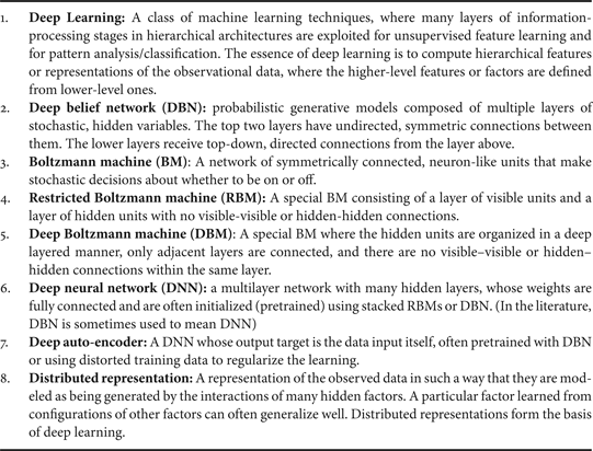
Table 1. Some basic deep learning terminologies.
A) Generative architectures
Associated with this generative category, we often see “unsupervised feature learning”, since the labels for the data are not of concern. When applying generative architectures to pattern recognition (i.e., supervised learning), a key concept here is (unsupervised) pretraining. This concept arises from the need to learn deep networks but learning the lower levels of such networks is difficult, especially when training data are limited. Therefore, it is desirable to learn each lower layer without relying on all the layers above and to learn all layers in a greedy, layer-by-layer manner from bottom up. This is the gist of “pretraining” before subsequent learning of all layers together.
Among the various subclasses of generative deep architecture, the energy-based deep models including autoencoders are the most common (e.g., [Reference Bengio4, Reference LeCun, Chopra, Ranzato and Huang35–Reference Ngiam, Chen, Koh and Ng38]). The original form of the deep autoencoder [Reference Hinton and Salakhutdinov21, Reference Deng, Seltzer, Yu, Acero, Mohamed and Hinton30], which we will give more detail about in Section IV, is a typical example in the generative model category. Most other forms of deep autoencoders are also generative in nature, but with quite different properties and implementations. Examples are transforming autoencoders [Reference Hinton, Krizhevsky and Wang39], predictive sparse coders and their stacked version, and denoising autoencoders and their stacked versions [Reference Vincent, Larochelle, Lajoie, Bengio and Manzagol27].
Specifically, in denoising autoencoders, the input vectors are first corrupted; e.g., randomizing a percentage of the inputs and setting them to zeros. Then one designs the hidden encoding nodes to reconstruct the original, uncorrupted input data using criteria such as KL distance between the original inputs and the reconstructed inputs. Uncorrupted encoded representations are used as the inputs to the next level of the stacked denoising autoencoder.
Another prominent type of generative model is deep Boltzmann machine or DBM [Reference Salakhutdinov and Hinton40–Reference Srivastava and Salakhutdinov42]. A DBM contains many layers of hidden variables, and has no connections between the variables within the same layer. This is a special case of the general Boltzmann machine (BM), which is a network of symmetrically connected units that make stochastic decisions about whether to be on or off. While having very simple learning algorithm, the general BMs are very complex to study and very slow to compute in learning. In a DBM, each layer captures complicated, higher-order correlations between the activities of hidden features in the layer below. DBMs have the potential of learning internal representations that become increasingly complex, highly desirable for solving object and speech recognition problems. Furthermore, the high-level representations can be built from a large supply of unlabeled sensory inputs and very limited labeled data can then be used to only slightly fine-tune the model for a specific task at hand.
When the number of hidden layers of DBM is reduced to one, we have RBM. Like DBM, there are no hidden-to-hidden and no visible-to-visible connections. The main virtue of RBM is that via composing many RBMs, many hidden layers can be learned efficiently using the feature activations of one RBM as the training data for the next. Such composition leads to DBN, which we will describe in more detail, together with RBMs, in Section V.
The standard DBN has been extended to the factored higher-order BM in its bottom layer, with strong results for phone recognition obtained [Reference Dahl, Ranzato, Mohamed and Hinton43]. This model, called mean-covariance RBM or mcRBM, recognizes the limitation of the standard RBM in its ability to represent the covariance structure of the data. However, it is very difficult to train mcRBM and to use it at the higher levels of the deep architecture. Furthermore, the strong results published are not easy to reproduce. In the architecture of [Reference Dahl, Ranzato, Mohamed and Hinton43], the mcRBM parameters in the full DBN are not easy to be fine-tuned using the discriminative information as for the regular RBMs in the higher layers. However, recent work showed that when better features are used, e.g., cepstral speech features subject to linear discriminant analysis or to fMLLR transformation, then the mcRBM is not needed as covariance in the transformed data is already modeled [Reference Mohamed, Hinton and Penn26].
Another representative deep generative architecture is the sum-product network or SPN [Reference Poon and Domingos44, Reference Gens and Domingo45]. An SPN is a directed acyclic graph with the data as leaves, and with sum and product operations as internal nodes in the deep architecture. The “sum” nodes give mixture models, and the “product” nodes build up the feature hierarchy. Properties of “completeness” and “consistency” constrain the SPN in a desirable way. The learning of SPN is carried out using the EM algorithm together with backpropagation. The learning procedure starts with a dense SPN. It then finds an SPN structure by learning its weights, where zero weights remove the connections. The main difficulty in learning is found to be the common one – the learning signal (i.e., the gradient) quickly dilutes when it propagates to deep layers. Empirical solutions have been found to mitigate this difficulty reported in [Reference Poon and Domingos44], where it was pointed out that despite the many desirable generative properties in the SPN, it is difficult to fine tune its weights using the discriminative information, limiting its effectiveness in classification tasks. This difficulty has been overcome in the subsequent work reported in [Reference Gens and Domingo45], where an efficient backpropagation-style discriminative training algorithm for SPN was presented. It was pointed out that the standard gradient descent, computed by the derivative of the conditional likelihood, suffers from the same gradient diffusion problem well known for the regular deep networks. But when marginal inference is replaced by inferring the most probable state of the hidden variables, such a “hard” gradient descent can reliably estimate deep SPNs' weights. Excellent results on (small-scale) image recognition tasks are reported.
RNNs can be regarded as a class of deep generative architectures when they are used to model and generate sequential data (e.g., [Reference Sutskever, Martens and Hinton46]). The “depth” of an RNN can be as large as the length of the input data sequence. RNNs are very powerful for modeling sequence data (e.g., speech or text), but until recently they had not been widely used partly because they are extremely difficult to train properly due to the well-known “vanishing gradient” problem. Recent advances in Hessian-free optimization [Reference Martens47] have partially overcome this difficulty using second-order information or stochastic curvature estimates. In the recent work of [Reference Martens and Sutskever48], RNNs that are trained with Hessian-free optimization are used as a generative deep architecture in the character-level language modeling (LM) tasks, where gated connections are introduced to allow the current input characters to predict the transition from one latent state vector to the next. Such generative RNN models are demonstrated to be well capable of generating sequential text characters. More recently, Bengio et al. [Reference Bengio, Boulanger and Pascanu49] and Sutskever [Reference Sutskever50] have explored new optimization methods in training generative RNNs that modify stochastic gradient descent and show these modifications can outperform Hessian-free optimization methods. Mikolov et al. [Reference Mikolov, Karafiat, Burget, Cernocky and Khudanpur51] have reported excellent results on using RNNs for LM. More recently, Mesnil et al. [Reference Mesnil, He, Deng and Bengio52] reported the success of RNNs in spoken language understanding.
As examples of a different type of generative deep models, there has been a long history in speech recognition research where human speech production mechanisms are exploited to construct dynamic and deep structure in probabilistic generative models; for a comprehensive review, see book [Reference Deng53]. Specifically, the early work described in [Reference Deng54–Reference Deng and Aksmanovic59] generalized and extended the conventional shallow and conditionally independent HMM structure by imposing dynamic constraints, in the form of polynomial trajectory, on the HMM parameters. A variant of this approach has been more recently developed using different learning techniques for time-varying HMM parameters and with the applications extended to speech recognition robustness [Reference Yu and Deng60, Reference Yu, Deng, Gong and Acero61]. Similar trajectory HMMs also form the basis for parametric speech synthesis [Reference Zen, Nankaku and Tokuda62–Reference Shannon, Zen and Byrne66]. Subsequent work added a new hidden layer into the dynamic model so as to explicitly account for the target-directed, articulatory-like properties in human speech generation [Reference Deng15, Reference Deng16, Reference Deng, Ramsay and Sun67–Reference Ma and Deng73]. More efficient implementation of this deep architecture with hidden dynamics is achieved with non-recursive or FIR filters in more recent studies [Reference Deng, Yu and Acero74–Reference Deng and Yu76]. The above deep-structured generative models of speech can be shown as special cases of the more general dynamic Bayesian network model and even more general dynamic graphical models [Reference Bilmes and Bartels77, Reference Bilmes78]. The graphical models can comprise many hidden layers to characterize the complex relationship between the variables in speech generation. Armed with powerful graphical modeling tool, the deep architecture of speech has more recently been successfully applied to solve the very difficult problem of single-channel, multi-talker speech recognition, where the mixed speech is the visible variable while the un-mixed speech becomes represented in a new hidden layer in the deep generative architecture [Reference Rennie, Hershey and Olsen79, Reference Wohlmayr, Stark and Pernkopf80]. Deep generative graphical models are indeed a powerful tool in many applications due to their capability of embedding domain knowledge. However, in addition to the weakness of using non-distributed representations for the classification categories, they also are often implemented with inappropriate approximations in inference, learning, prediction, and topology design, all arising from inherent intractability in these tasks for most real-world applications. This problem has been partly addressed in the recent work of [Reference Stoyanov, Ropson and Eisner81], which provides an interesting direction for making deep generative graphical models potentially more useful in practice in the future.
The standard statistical methods used for large-scale speech recognition and understanding combine (shallow) HMMs for speech acoustics with higher layers of structure representing different levels of natural language hierarchy. This combined hierarchical model can be suitably regarded as a deep generative architecture, whose motivation and some technical detail may be found in Chapter 7 in the recent book [Reference Kurzweil82] on “Hierarchical HMM” or HHMM. Related models with greater technical depth and mathematical treatment can be found in [Reference Fine, Singer and Tishby83] for HHMM and [Reference Oliver, Garg and Horvitz84] for Layered HMM. These early deep models were formulated as directed graphical models, missing the key aspect of “distributed representation” embodied in the more recent deep generative architectures of DBN and DBM discussed earlier in this section.
Finally, temporally recursive and deep generative models can be found in [Reference Taylor, Hinton and Roweis85] for human motion modeling, and in [Reference Socher, Lin, Ng and Manning86] for natural language and natural scene parsing. The latter model is particularly interesting because the learning algorithms are capable of automatically determining the optimal model structure. This contrasts with other deep architectures such as the DBN where only the parameters are learned while the architectures need to be predefined. Specifically, as reported in [Reference Socher, Lin, Ng and Manning86], the recursive structure commonly found in natural scene images and in natural language sentences can be discovered using a max-margin structure prediction architecture. Not only the units contained in the images or sentences are identified but so is the way in which these units interact with each other to form the whole.
B) Discriminative architectures
Many of the discriminative techniques in signal and information processing apply to shallow architectures such as HMMs (e.g., [Reference Juang, Chou and Lee87–Reference Gibson and Hain94]) or CRFs (e.g., [Reference Yang and Furui95–Reference Peng, Bo and Xu100]). Since a CRF is defined with the conditional probability on input data as well as on the output labels, it is intrinsically a shallow discriminative architecture. (Interesting equivalence between CRF and discriminatively trained Gaussian models and HMMs can be found in [Reference Heigold, Ney, Lehnen, Gass and Schluter101]. More recently, deep-structured CRFs have been developed by stacking the output in each lower layer of the CRF, together with the original input data, onto its higher layer [Reference Yu, Wang and Deng96]. Various versions of deep-structured CRFs are usefully applied to phone recognition [Reference Yu and Deng102], spoken language identification [Reference Yu, Wang, Karam and Deng103], and natural language processing [Reference Yu, Wang and Deng96]. However, at least for the phone recognition task, the performance of deep-structured CRFs, which is purely discriminative (non-generative), has not been able to match that of the hybrid approach involving DBN, which we will take on shortly.
The recent article of [Reference Morgan33] gives an excellent review on other major existing discriminative models in speech recognition based mainly on the traditional neural network or MLP architecture using backpropagation learning with random initialization. It argues for the importance of both the increased width of each layer of the neural networks and the increased depth. In particular, a class of DNN models forms the basis of the popular “tandem” approach, where a discriminatively learned neural network is developed in the context of computing discriminant emission probabilities for HMMs. For some representative recent works in this area, see [Reference Pinto, Garimella, Magimai-Doss, Hermansky and Bourlard104, Reference Ketabdar and Bourlard105]. The tandem approach generates discriminative features for an HMM by using the activities from one or more hidden layers of a neural network with various ways of information combination, which can be regarded as a form of discriminative deep architectures [Reference Morgan33, Reference Morgan106].
In the most recent work of [Reference Deng, Yu and Platt108–Reference Lena, Nagata and Baldi110], a new deep learning architecture, sometimes called DSN, together with its tensor variant [Reference Hutchinson, Deng and Yu111, Reference Hutchinson, Deng and Yu112] and its kernel version [Reference Deng, Tur, He and Hakkani-Tur11], are developed that all focus on discrimination with scalable, parallelizable learning relying on little or no generative component. We will describe this type of discriminative deep architecture in detail in Section V.
RNNs have been successfully used as a generative model when the “output” is taken to be the predicted input data in the future, as discussed in the preceding subsection; see also the neural predictive model [Reference Deng, Hassanein and Elmasry113] with the same mechanism. They can also be used as a discriminative model where the output is an explicit label sequence associated with the input data sequence. Note that such discriminative RNNs were applied to speech a long time ago with limited success (e.g., [Reference Robinson114]). For training RNNs for discrimination, presegmented training data are typically required. Also, post-processing is needed to transform their outputs into label sequences. It is highly desirable to remove such requirements, especially the costly presegmentation of training data. Often a separate HMM is used to automatically segment the sequence during training, and to transform the RNN classification results into label sequences [Reference Robinson114]. However, the use of HMM for these purposes does not take advantage of the full potential of RNNs.
An interesting method was proposed in [Reference Graves, Fernandez, Gomez and Schmidhuber115–Reference Graves117] that enables the RNNs themselves to perform sequence classification, removing the need for presegmenting the training data and for post-processing the outputs. Underlying this method is the idea of interpreting RNN outputs as the conditional distributions over all possible label sequences given the input sequences. Then, a differentiable objective function can be derived to optimize these conditional distributions over the correct label sequences, where no segmentation of data is required.
Another type of discriminative deep architecture is convolutional neural network (CNN), with each module consisting of a convolutional layer and a pooling layer. These modules are often stacked up with one on top of another, or with a DNN on top of it, to form a deep model. The convolutional layer shares many weights, and the pooling layer subsamples the output of the convolutional layer and reduces the data rate from the layer below. The weight sharing in the convolutional layer, together with appropriately chosen pooling schemes, endows the CNN with some “invariance” properties (e.g., translation invariance). It has been argued that such limited “invariance” or equi-variance is not adequate for complex pattern recognition tasks and more principled ways of handling a wider range of invariance are needed [Reference Hinton, Krizhevsky and Wang39]. Nevertheless, the CNN has been found highly effective and been commonly used in computer vision and image recognition [Reference LeCun, Bottou, Bengio and Haffner118–Reference Krizhevsky, Sutskever and Hinton121, Reference Le, Ranzato, Monga, Devin, Corrado, Chen, Dean and Ng154]. More recently, with appropriate changes from the CNN designed for image analysis to that taking into account speech-specific properties, the CNN is also found effective for speech recognition [Reference Abdel-Hamid, Mohamed, Jiang and Penn122–Reference Deng, Abdel-Hamid and Yu126]. We will discuss such applications in more detail in Section VII.
It is useful to point out that time-delay neural networks (TDNN, [,127129]) developed for early speech recognition are a special case of the CNN when weight sharing is limited to one of the two dimensions, i.e., time dimension. It was not until recently that researchers have discovered that time is the wrong dimension to impose “invariance” and frequency dimension is more effective in sharing weights and pooling outputs [Reference Abdel-Hamid, Mohamed, Jiang and Penn122, Reference Abdel-Hamid, Deng and Yu123, Reference Deng, Abdel-Hamid and Yu126]. An analysis on the underlying reasons are provided in [Reference Deng, Abdel-Hamid and Yu126], together with a new strategy for designing the CNN's pooling layer demonstrated to be more effective than nearly all previous CNNs in phone recognition.
It is also useful to point out that the model of hierarchical temporal memory (HTM, [Reference George17, Reference Hawkins and Blakeslee128, Reference Hawkins, Ahmad and Dubinsky130] is another variant and extension of the CNN. The extension includes the following aspects: (1) Time or temporal dimension is introduced to serve as the “supervision” information for discrimination (even for static images); (2) both bottom-up and top-down information flow are used, instead of just bottom-up in the CNN; and (3) a Bayesian probabilistic formalism is used for fusing information and for decision making.
Finally, the learning architecture developed for bottom-up, detection-based speech recognition proposed in [Reference Lee131] and developed further since 2004, notably in [Reference Yu, Siniscalchi, Deng and Lee132–Reference Siniscalchi, Svendsen and Lee134] using the DBN–DNN technique, can also be categorized in the discriminative deep architecture category. There is no intent and mechanism in this architecture to characterize the joint probability of data and recognition targets of speech attributes and of the higher-level phone and words. The most current implementation of this approach is based on multiple layers of neural networks using backpropagation learning [Reference Yu, Seide, Li and Deng135]. One intermediate neural network layer in the implementation of this detection-based framework explicitly represents the speech attributes, which are simplified entities from the “atomic” units of speech developed in the early work of [Reference Deng and Sun136, Reference Sun and Deng137]. The simplification lies in the removal of the temporally overlapping properties of the speech attributes or articulatory-like features. Embedding such more realistic properties in the future work is expected to improve the accuracy of speech recognition further.
C) Hybrid generative–discriminative architectures
The term “hybrid” for this third category refers to the deep architecture that either comprises or makes use of both generative and discriminative model components. In many existing hybrid architectures published in the literature (e.g., [Reference Hinton and Salakhutdinov21, Reference Mohamed, Yu and Deng23, Reference Dahl, Yu, Deng and Acero25, Reference Sainath, Kingsbury and Ramabhadran138]), the generative component is exploited to help with discrimination, which is the final goal of the hybrid architecture. How and why generative modeling can help with discrimination can be examined from two viewpoints:
-
(1) The optimization viewpoint where generative models can provide excellent initialization points in highly non-linear parameter estimation problems (the commonly used term of “pretraining” in deep learning has been introduced for this reason); and/or
-
(2) The regularization perspective where generative models can effectively control the complexity of the overall model.
The study reported in [Reference Erhan, Bengio, Courvelle, Manzagol, Vencent and Bengio139] provided an insightful analysis and experimental evidence supporting both of the viewpoints above.
When the generative deep architecture of DBN discussed in Section III-A is subject to further discriminative training using backprop, commonly called “fine-tuning” in the literature, we obtain an equivalent architecture of the DNN. The weights of the DNN can be “pretrained” from stacked RBMs or DBN instead of the usual random initialization. See [Reference Mohamed, Dahl and Hinton24] for a detailed explanation of the equivalence relationship and the use of the often confusing terminology. We will review details of the DNN in the context of RBM/DBN pretraining as well as its interface with the most commonly used shallow generative architecture of HMM (DNN–HMM) in Section IV.
Another example of the hybrid deep architecture is developed in [Reference Mohamed, Yu and Deng23], where again the generative DBN is used to initialize the DNN weights but the fine tuning is carried out not using frame-level discriminative information (e.g., cross-entropy error criterion) but sequence-level one. This is a combination of the static DNN with the shallow discriminative architecture of CRF. Here, the overall architecture of DNN–CRF is learned using the discriminative criterion of the conditional probability of full label sequences given the input sequence data. It can be shown that such DNN–CRF is equivalent to a hybrid deep architecture of DNN and HMM whose parameters are learned jointly using the full-sequence maximum mutual information (MMI) between the entire label sequence and the input vector sequence. A closely related full-sequence training method is carried out with success for a shallow neural network [Reference Kingsbury140] and for a deep one [Reference Kingsbury, Sainath and Soltau141].
Here, it is useful to point out a connection between the above hybrid discriminative training and a highly popular minimum phone error (MPE) training technique for the HMM [Reference Povey and Woodland89]. In the iterative MPE training procedure using extended Baum–Welch, the initial HMM parameters cannot be arbitrary. One commonly used initial parameter set is that trained generatively using Baum–Welch algorithm for maximum likelihood. Furthermore, an interpolation term taking the values of generatively trained HMM parameters is needed in the extended Baum–Welch updating formula, which may be analogous to “fine tuning” in the DNN training discussed earlier. Such I-smoothing [Reference Povey and Woodland89] has a similar spirit to DBN pretraining in the “hybrid” DNN learning.
Along the line of using discriminative criteria to train parameters in generative models as in the above HMM training example, we here briefly discuss the same method applied to learning other generative architectures. In [Reference Larochelle and Bengio142], the generative model of RBM is learned using the discriminative criterion of posterior class/label probabilities when the label vector is concatenated with the input data vector to form the overall visible layer in the RBM. In this way, RBM can be considered as a stand-alone solution to classification problems and the authors derived a discriminative learning algorithm for RBM as a shallow generative model. In the more recent work of [Reference Ranzato, Susskind, Mnih and Hinton146], the deep generative model of DBN with the gated MRF at the lowest level is learned for feature extraction and then for recognition of difficult image classes including occlusions. The generative ability of the DBN model facilitates the discovery of what information is captured and what is lost at each level of representation in the deep model, as demonstrated in [Reference Ranzato, Susskind, Mnih and Hinton146]. A related work on using the discriminative criterion of empirical risk to train deep graphical models can be found in [Reference Stoyanov, Ropson and Eisner81].
A further example of the hybrid deep architecture is the use of the generative model of DBN to pretrain deep convolutional neural networks (deep DNN) [Reference Abdel-Hamid, Deng and Yu123, Reference Lee, Grosse, Ranganath and Ng144, Reference Lee, Largman, Pham and Ng145]). Like the fully-connected DNN discussed earlier, the DBN pretraining is also shown to improve discrimination of the deep CNN over random initialization.
The final example given here of the hybrid deep architecture is based on the idea and work of [Reference Ney147, Reference He and Deng148], where one task of discrimination (speech recognition) produces the output (text) that serves as the input to the second task of discrimination (machine translation). The overall system, giving the functionality of speech translation – translating speech in one language into text in another language – is a two-stage deep architecture consisting of both generative and discriminative elements. Both models of speech recognition (e.g., HMM) and of machine translation (e.g., phrasal mapping and non-monotonic alignment) are generative in nature. But their parameters are all learned for discrimination. The framework described in [Reference He and Deng148] enables end-to-end performance optimization in the overall deep architecture using the unified learning framework initially published in [Reference He, Deng and Chou90]. This hybrid deep learning approach can be applied to not only speech translation but also all speech-centric and possibly other information-processing tasks such as speech information retrieval, speech understanding, cross-lingual speech/text understanding and retrieval, etc. (e.g., [Reference Deng, Tur, He and Hakkani-Tur11, Reference Tur, Deng, Hakkani-Tür and He109, Reference Yamin, Deng, Wang and Acero149–Reference He, Deng, Tur and Hakkani-Tur153]).
After briefly surveying a wide range of work in each of the three classes of deep architectures above, in the following three sections, I will elaborate on three prominent models of deep learning, one from each of the three classes. While ideally they should represent the most influential architectures giving state of the art performance, I have chosen the three that I am most familiar with as being responsible for their developments and that may serve the tutorial purpose well with the simplicity of the architectural and mathematical descriptions. The three architectures described in the following three sections may not be interpreted as the most representative and influential work in each of the three classes. For example, in the category of generative architectures, the highly complex deep architecture and generative training methods developed by and described in [Reference Le, Ranzato, Monga, Devin, Corrado, Chen, Dean and Ng154], which is beyond the scope of this tutorial, performs quite well in image recognition. Likewise, in the category of discriminative architectures, the even more complex architecture and learning described in Kingsbury et al. [Reference Kingsbury, Sainath and Soltau141], Seide et al. [Reference Seide, Li and Yu155], and Yan et al. [Reference Yan, Huo and Xu156] gave the state of the art performance in large-scale speech recognition.
IV. GENERATIVE ARCHITECTURE: DEEP AUTOENCODER
A) Introduction
Deep autoencoder is a special type of DNN whose output is the data input itself, and is used for learning efficient encoding or dimensionality reduction for a set of data. More specifically, it is a non-linear feature extraction method involving no class labels; hence generative. An autoencoder uses three or more layers in the neural network:
-
• An input layer of data to be efficiently coded (e.g., pixels in image or spectra in speech);
-
• One or more considerably smaller hidden layers, which will form the encoding.
-
• An output layer, where each neuron has the same meaning as in the input layer.
When the number of hidden layers is greater than one, the autoencoder is considered to be deep.
An autoencoder is often trained using one of the many backpropagation variants (e.g., conjugate gradient method, steepest descent, etc.) Though often reasonably effective, there are fundamental problems with using backpropagation to train networks with many hidden layers. Once the errors get backpropagated to the first few layers, they become minuscule, and quite ineffective. This causes the network to almost always learn to reconstruct the average of all the training data. Though more advanced backpropagation methods (e.g., the conjugate gradient method) help with this to some degree, it still results in very slow learning and poor solutions. This problem is remedied by using initial weights that approximate the final solution. The process to find these initial weights is often called pretraining.
A successful pretraining technique developed in [Reference Hinton, Osindero and Teh3] for training deep autoencoders involves treating each neighboring set of two layers such as an RBM for pretraining to approximate a good solution and then using a backpropagation technique to fine-tune so as the minimize the “coding” error. This training technique is applied to construct a deep autoencoder to map images to short binary code for fast, content-based image retrieval. It is also applied to coding documents (called semantic hashing), and to coding spectrogram-like speech features, which we review below.
B) Use of deep autoencoder to extract speech features
Here we review the more recent work of [Reference Deng, Seltzer, Yu, Acero, Mohamed and Hinton30] in developing a similar type of autoencoder for extracting bottleneck speech instead of image features. Discovery of efficient binary codes related to such features can also be used in speech information retrieval. Importantly, the potential benefits of using discrete representations of speech constructed by this type of deep autoencoder can be derived from an almost unlimited supply of unlabeled data in future-generation speech recognition and retrieval systems.
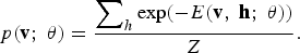
A deep generative model of patches of spectrograms that contain 256 frequency bins and 1, 3, 9, or 13 frames is illustrated in Fig. 1. An undirected graphical model called a Gaussian-binary RBM is built that has one visible layer of linear variables with Gaussian noise and one hidden layer of 500–3000 binary latent variables. After learning the Gaussian-binary RBM, the activation probabilities of its hidden units are treated as the data for training another binary–binary RBM. These two RBMs can then be composed to form a DBN in which it is easy to infer the states of the second layer of binary hidden units from the input in a single forward pass. The DBN used in this work is illustrated on the left side of Fig. 1, where the two RBMs are shown in separate boxes. (See more detailed discussions on RBM and DBN in the next section.)
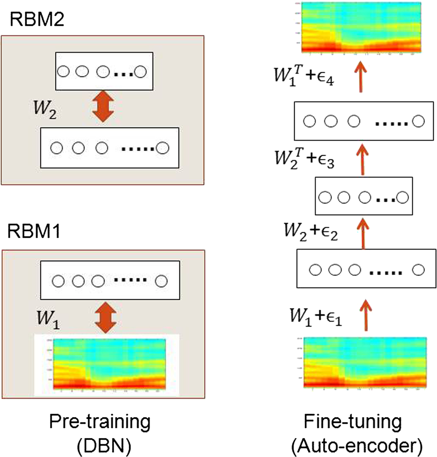
Fig. 1. The architecture of the deep autoencoder used in [30] for extracting “bottle-neck” speech features from high-resolution spectrograms.
The deep autoencoder with three hidden layers is formed by “unrolling” the DBN using its weight matrices. The lower layers of this deep autoencoder use the matrices to encode the input and the upper layers use the matrices in reverse order to decode the input. This deep autoencoder is then fine-tuned using backpropagation of error-derivatives to make its output as similar as possible to its input, as shown on the right side of Fig. 1. After learning is complete, any variable-length spectrogram can be encoded and reconstructed as follows. First, N-consecutive overlapping frames of 256-point log power spectra are each normalized to zero-mean and unit-variance to provide the input to the deep autoencoder. The first hidden layer then uses the logistic function to compute real-valued activations. These real values are fed to the next, coding layer to compute “codes”. The real-valued activations of hidden units in the coding layer are quantized to be either zero or one with 0.5 as the threshold. These binary codes are then used to reconstruct the original spectrogram, where individual fixed-frame patches are reconstructed first using the two upper layers of network weights. Finally, overlap-and-add technique is used to reconstruct the full-length speech spectrogram from the outputs produced by applying the deep autoencoder to every possible window of N consecutive frames. We show some illustrative encoding and reconstruction examples below.
C) Illustrative examples
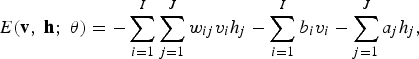
At the top of Fig. 2 is the original speech, followed by the reconstructed speech utterances with forced binary values (zero or one) at the 312 unit code layer for encoding window lengths of N = 1, 3, 9, and 13, respectively. The lower coding errors for N = 9 and 13 are clearly seen.
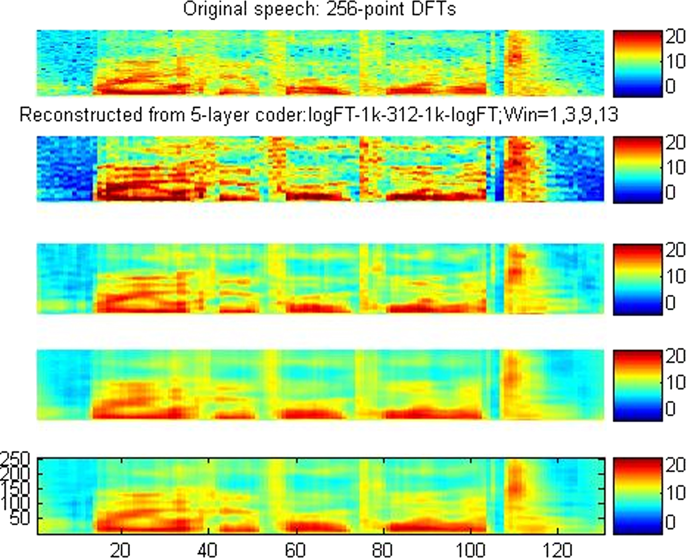
Fig. 2. Top to Bottom: Original spectrogram; reconstructions using input window sizes of N = 1, 3, 9, and 13 while forcing the coding units to be zero or one (i.e., a binary code). The y-axis values indicate FFT bin numbers (i.e., 256-point FFT is used for constructing all spectrograms).
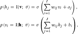
Encoding accuracy of the deep autoencoder is qualitatively examined to compare with the more traditional codes via vector quantization (VQ). Figure 3 shows various aspects of the encoding accuracy. At the top is the original speech utterance's spectrogram. The next two spectrograms are the blurry reconstruction from the 312-bit VQ and the much more faithful reconstruction from the 312-bit deep autoencoder. Coding errors from both coders, plotted as a function of time, are shown below the spectrograms, demonstrating that the autoencoder (red curve) is producing lower errors than the VQ coder (blue curve) throughout the entire span of the utterance. The final two spectrograms show the detailed coding error distributions over both time and frequency bins.

Fig. 3. Top to bottom: Original spectrogram from the test set; reconstruction from the 312-bit VQ coder; reconstruction from the 312-bit autoencoder; coding errors as a function of time for the VQ coder (blue) and autoencoder (red); spectrogram of the VQ coder residual; spectrogram of the deep autoencoder's residual.
D) Transforming autoencoder
The deep autoencoder described above can extract a compact code for a feature vector due to its many layers and the non-linearity. But the extracted code would change unpredictably when the input feature vector is transformed. It is desirable to be able to have the code change predictably that reflects the underlying transformation invariant to the perceived content. This is the goal of transforming autoencoder proposed in for image recognition [Reference Hinton, Krizhevsky and Wang39].
The building block of the transforming autoencoder is a “capsule”, which is an independent subnetwork that extracts a single parameterized feature representing a single entity, be it visual or audio. A transforming autoencoder receives both an input vector and a target output vector, which is related to the input vector by a simple global transformation; e.g., the translation of a whole image or frequency shift due to vocal tract length differences for speech. An explicit representation of the global transformation is known also. The bottleneck or coding layer of the transforming autoencoder consists of the outputs of several capsules.
During the training phase, the different capsules learn to extract different entities in order to minimize the error between the final output and the target.
In addition to the deep autoencoder architectures described in this section, there are many other types of generative architectures in the literature, all characterized by the use of data alone (i.e., free of classification labels) to automatically derive higher-level features. Although such more complex architectures have produced state of the art results (e.g., [Reference Le, Ranzato, Monga, Devin, Corrado, Chen, Dean and Ng154]), their complexity does not permit detailed treatment in this tutorial paper; rather, a brief survey of a broader range of the generative deep architectures was included in Section III-A.
V. HYBRID ARCHITECTURE: DNN PRETRAINED WITH DBN
A) Basics
In this section, we present the most widely studied hybrid deep architecture of DNNs, consisting of both pretraining (using generative DBN) and fine-tuning stages in its parameter learning. Part of this review is based on the recent publication of [Reference Hinton6, Reference Yu and Deng7, Reference Dahl, Yu, Deng and Acero25].
As the generative component of the DBN, it is a probabilistic model composed of multiple layers of stochastic, latent variables. The unobserved variables can have binary values and are often called hidden units or feature detectors. The top two layers have undirected, symmetric connections between them and form an associative memory. The lower layers receive top-down, directed connections from the layer above. The states of the units in the lowest layer, or the visible units, represent an input data vector.
There is an efficient, layer-by-layer procedure for learning the top-down, generative weights that determine how the variables in one layer depend on the variables in the layer above. After learning, the values of the latent variables in every layer can be inferred by a single, bottom-up pass that starts with an observed data vector in the bottom layer and uses the generative weights in the reverse direction.
DBNs are learned one layer at a time by treating the values of the latent variables in one layer, when they are being inferred from data, as the data for training the next layer. This efficient, greedy learning can be followed by, or combined with, other learning procedures that fine-tune all of the weights to improve the generative or discriminative performance of the full network. This latter learning procedure constitutes the discriminative component of the DBN as the hybrid architecture.
Discriminative fine-tuning can be performed by adding a final layer of variables that represent the desired outputs and backpropagating error derivatives. When networks with many hidden layers are applied to highly structured input data, such as speech and images, backpropagation works much better if the feature detectors in the hidden layers are initialized by learning a DBN to model the structure in the input data as originally proposed in [Reference Hinton and Salakhutdinov21].
A DBN can be viewed as a composition of simple learning modules via stacking them. This simple learning module is called RBMs that we introduce next.
B) Restricted BM
An RBM is a special type of Markov random field that has one layer of (typically Bernoulli) stochastic hidden units and one layer of (typically Bernoulli or Gaussian) stochastic visible or observable units. RBMs can be represented as bipartite graphs, where all visible units are connected to all hidden units, and there are no visible–visible or hidden–hidden connections.
In an RBM, the joint distribution p(v, h; θ) over the visible units v and hidden units h, given the model parameters θ, is defined in terms of an energy function E(v, h; θ) of
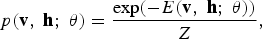 $$p \lpar {\bf v}\comma \; {\bf h}\semicolon \; \theta\rpar = {\displaystyle{{\rm exp} \lpar -E\lpar {\bf v}\comma \; {\bf h}\semicolon \; \theta\rpar \rpar } \over{Z}}\comma \;$$
where Z = ∑ v ∑ h exp (−E(v, h; θ)) is a normalization factor or partition function, and the marginal probability that the model assigns to a visible vector v is
 $$p\lpar {\bf v}\semicolon \; \theta\rpar = {\displaystyle{\sum \nolimits_h {\rm exp} \lpar -E\lpar {\bf v}\comma \; {\bf h}\semicolon \; \theta\rpar \rpar } \over {Z}}.$$
For a Bernoulli (visible)–Bernoulli (hidden) RBM, the energy function is defined as
 $$E\lpar {\bf v}\comma \; {\bf h}\semicolon \; \theta\rpar = - \sum_{i=1}^I \sum_{j=1}^J w_{ij} v_i h_{\!j} - \sum_{i=1}^I b_i v_i - \sum_{j=1}^J a_j h_{\!j}\comma \;$$
where w ij represents the symmetric interaction term between visible unit v i and hidden unit h j , b i and a j the bias terms, and I and J are the numbers of visible and hidden units. The conditional probabilities can be efficiently calculated as
 $$\eqalign{&p\lpar h_{j} = 1\vert {\bf v}\semicolon \; \theta\rpar = \sigma \left(\sum_{i=1}^I w_{ij} v_i +a_j\right)\comma \; \cr & p\lpar v_i = 1\vert {\bf h}\semicolon \; \theta\rpar = \sigma \left(\sum_{j=1}^J w_{ij} h_{j} +b_i\right)\comma \; }$$
where σ (x)=1/(1 + exp(x)).
Similarly, for a Gaussian (visible)–Bernoulli (hidden) RBM, the energy is
 $$\eqalign{E \lpar {\bf v}\comma \; {\bf h}\semicolon \; \theta\rpar = &- \sum_{i=1}^I \sum_{j=1}^J w_{ij} v_i h_{j} \cr & - {\displaystyle {1} \over {2}} \sum_{i=1}^I \lpar v_i -b_i\rpar ^2 - \sum_{j=1}^J a_j h_{j}\comma \; }$$
The corresponding conditional probabilities become
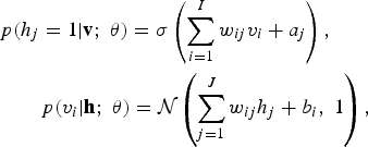 $$\eqalign{& p\lpar h_{j} = 1\vert {\bf v}\semicolon \; \theta\rpar = \sigma \left(\sum_{i=1}^I w_{ij} v_i + a_j\right)\comma \; \cr & \quad \quad p\lpar v_i \vert {\bf h}\semicolon \; \theta\rpar = {\cal N} \left(\sum_{j=1}^J w_{ij} h_{j} + b_i\comma \; 1\right)\comma \; }$$
where v i takes real values and follows a Gaussian distribution with mean ∑ j=1 J w ij h j + b i and variance one. Gaussian–Bernoulli RBMs can be used to convert real-valued stochastic variables to binary stochastic variables, which can then be further processed using the Bernoulli–Bernoulli RBMs.
The above discussion used two most common conditional distributions for the visible data in the RBM – Gaussian (for continuous-valued data) and binomial (for binary data). More general types of distributions in the RBM can also be used. See [Reference Welling, Rosen-Zvi and Hinton157] for the use of general exponential-family distributions for this purpose.
Taking the gradient of the log likelihood log p (v; θ) we can derive the update rule for the RBM weights as:
 $$\Delta w_{ij} = E_{data} \lpar v_i h_{j}\rpar - E_{model} \lpar v_i h_{j}\rpar \comma \;$$
where E data (v i h j ) is the expectation observed in the training set and E model (v i h j ) is that same expectation under the distribution defined by the model. Unfortunately, E model (v i h j ) is intractable to compute so the contrastive divergence (CD) approximation to the gradient is used where E model (v i h j ) is replaced by running the Gibbs sampler initialized at the data for one full step. The steps in approximating E model (v i h j ) is as follows:
-
• Initialize v 0 at data
-
• Sample h 0 ~ p (h|v 0)
-
• Sample v 1 ~ p (v|h 0)
-
• Sample h 1 ~ p (h|v 1)
Then (v 1, h 1) is a sample from the model, as a very rough estimate of E model (v i h j ) = (v ∞, h ∞), which is a true sample from the model. Use of (v 1, h 1) to approximate E model (v i h j ) gives rise to the algorithm of CD-1. The sampling process can be pictorially depicted as below in Fig. 4 below.
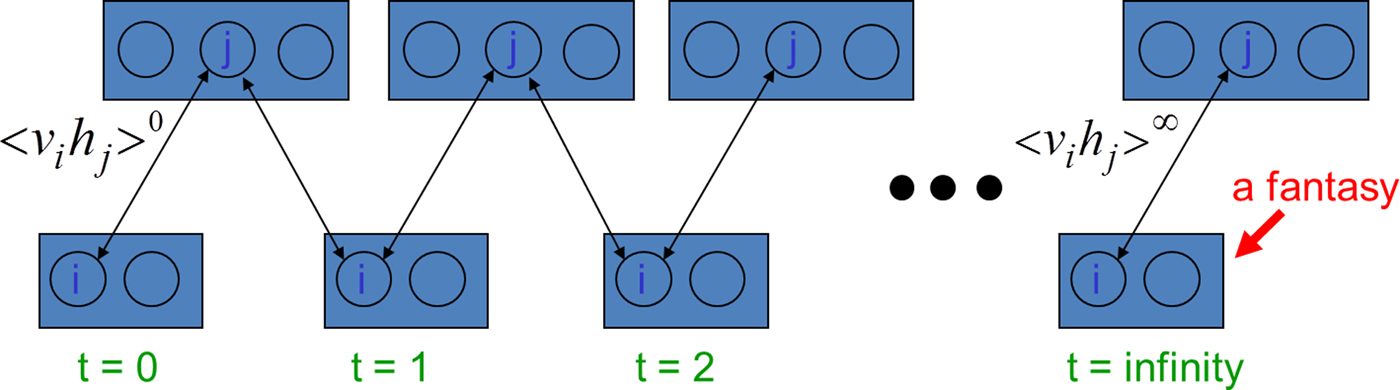
Fig. 4. A pictorial view of sampling from a RBM during the “negative” learning phase of the RBM (courtesy of G. Hinton).
Careful training of RBMs is essential to the success of applying RBM and related deep learning techniques to solve practical problems. See the Technical Report [Reference Hinton158] for a very useful practical guide for training RBMs.
The RBM discussed above is a generative model, which characterizes the input data distribution using hidden variables and there is no label information involved. However, when the label information is available, it can be used together with the data to form the joint “data” set. Then the same CD learning can be applied to optimize the approximate “generative” objective function related to data likelihood. Further, and more interestingly, a “discriminative” objective function can be defined in terms of conditional likelihood of labels. This discriminative RBM can be used to “fine tune” RBM for classification tasks [Reference Larochelle and Bengio142].
Note the SESM architecture by Ranzato et al. [Reference Ranzato, Boureau and LeCun29] surveyed in Section III is quite similar to the RBM described above. While they both have a symmetric encoder and decoder, and a logistic non-linearity on the top of the encoder, the main difference is that RBM is trained using (approximate) maximum likelihood, but SESM is trained by simply minimizing the average energy plus an additional code sparsity term. SESM relies on the sparsity term to prevent flat energy surfaces, while RBM relies on an explicit contrastive term in the loss, an approximation of the log partition function. Another difference is in the coding strategy in that the code units are “noisy” and binary in RBM, while they are quasi-binary and sparse in SESM.
C) Stacking up RBMs to form a DBN/DNN architecture
Stacking a number of the RBMs learned layer by layer from bottom up gives rise to a DBN, an example of which is shown in Fig. 5. The stacking procedure is as follows. After learning a Gaussian–Bernoulli RBM (for applications with continuous features such as speech) or Bernoulli–Bernoulli RBM (for applications with nominal or binary features such as black–white image or coded text), we treat the activation probabilities of its hidden units as the data for training the Bernoulli–Bernoulli RBM one layer up. The activation probabilities of the second-layer Bernoulli–Bernoulli RBM are then used as the visible data input for the third-layer Bernoulli–Bernoulli RBM, and so on. Some theoretical justifications of this efficient layer-by-layer greedy learning strategy is given in [Reference Hinton, Osindero and Teh3], where it is shown that the stacking procedure above improves a variational lower bound on the likelihood of the training data under the composite model. That is, the greedy procedure above achieves approximate maximum-likelihood learning. Note that this learning procedure is unsupervised and requires no class label.
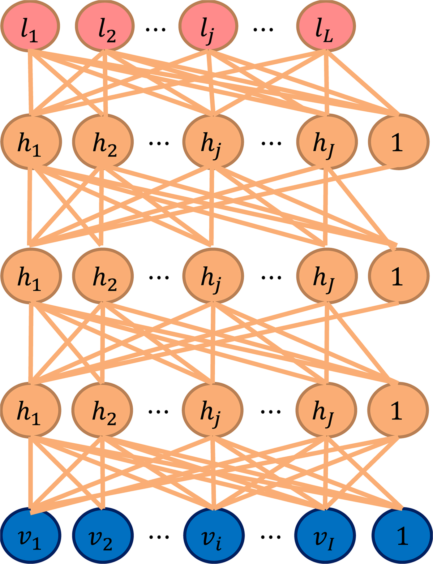
Fig. 5. Illustration of a DBN/DNN architecture.
When applied to classification tasks, the generative pretraining can be followed by or combined with other, typically discriminative, learning procedures that fine-tune all of the weights jointly to improve the performance of the network. This discriminative fine-tuning is performed by adding a final layer of variables that represent the desired outputs or labels provided in the training data. Then, the backpropagation algorithm can be used to adjust or fine-tune the DBN weights and use the final set of weights in the same way as for the standard feedforward neural network. What goes to the top, label layer of this DNN depends on the application. For speech recognition applications, the top layer, denoted by “l 1, l 2, … l j , …, l L ,” in Fig. 5, can represent either syllables, phones, subphones, phone states, or other speech units used in the HMM-based speech recognition system.
The generative pretraining described above has produced excellent phone and speech recognition results on a wide variety of tasks, which will be surveyed in Section VII. Further research has also shown the effectiveness of other pretraining strategies. As an example, greedy layer-by-layer training may be carried out with an additional discriminative term to the generative cost function at each level. And without generative pretraining, purely discriminative training of DNNs from random initial weights using the traditional stochastic gradient decent method has been shown to work very well when the scales of the initial weights are set carefully and the mini-batch sizes, which trade off noisy gradients with convergence speed, used in stochastic gradient decent are adapted prudently (e.g., with an increasing size over training epochs). Also, randomization order in creating mini-batches needs to be judiciously determined. Importantly, it was found effective to learn a DNN by starting with a shallow neural net with a single hidden layer. Once this has been trained discriminatively (using early stops to avoid overfitting), a second hidden layer is inserted between the first hidden layer and the labeled softmax output units and the expanded deeper network is again trained discriminatively. This can be continued until the desired number of hidden layers is reached, after which a full backpropagation “fine tuning” is applied. This discriminative “pretraining” procedure is found to work well in practice (e.g., [Reference Seide, Li and Yu155]).
This type of discriminative “pretraining” procedure is closely related to the learning algorithm developed for the deep architectures called deep convex/stacking network, to be described in Section VI, where interleaving linear and non-linear layers are used in building up the deep architectures in a modular manner, and the original input vectors are concatenated with the output vectors of each module consisting of a shallow neural net. Discriminative “pretraining” is used for positioning a subset of weights in each module in a reasonable space using parallelizable convex optimization, followed by a batch-mode “fine tuning” procedure, which is also parallelizable due to the closed-form constraint between two subsets of weights in each module.
Further, purely discriminative training of the full DNN from random initial weights is now known to work much better than had been thought in early days, provided that the scales of the initial weights are set carefully, a large amount of labeled training data is available, and mini-batch sizes over training epochs are set appropriately. Nevertheless, generative pretraining still improves test performance, sometimes by a significant amount especially for small tasks. Layer-by-layer generative pretraining was originally done using RBMs, but various types of autoencoder with one hidden layer can also be used.
D) Interfacing DNN with HMM
A DBN/DNN discussed above is a static classifier with input vectors having a fixed dimensionality. However, many practical pattern recognition and information-processing problems, including speech recognition, machine translation, natural language understanding, video processing and bio-information processing, require sequence recognition. In sequence recognition, sometimes called classification with structured input/output, the dimensionality of both inputs and outputs are variable.
The HMM, based on dynamic programming operations, is a convenient tool to help port the strength of a static classifier to handle dynamic or sequential patterns. Thus, it is natural to combine DBN/DNN and HMM to bridge the gap between static and sequence pattern recognition. An architecture that shows the interface between a DNN and HMM is provided in Fig. 6. This architecture has been successfully used in speech recognition experiments as reported in [Reference Dahl, Yu, Deng and Acero25].
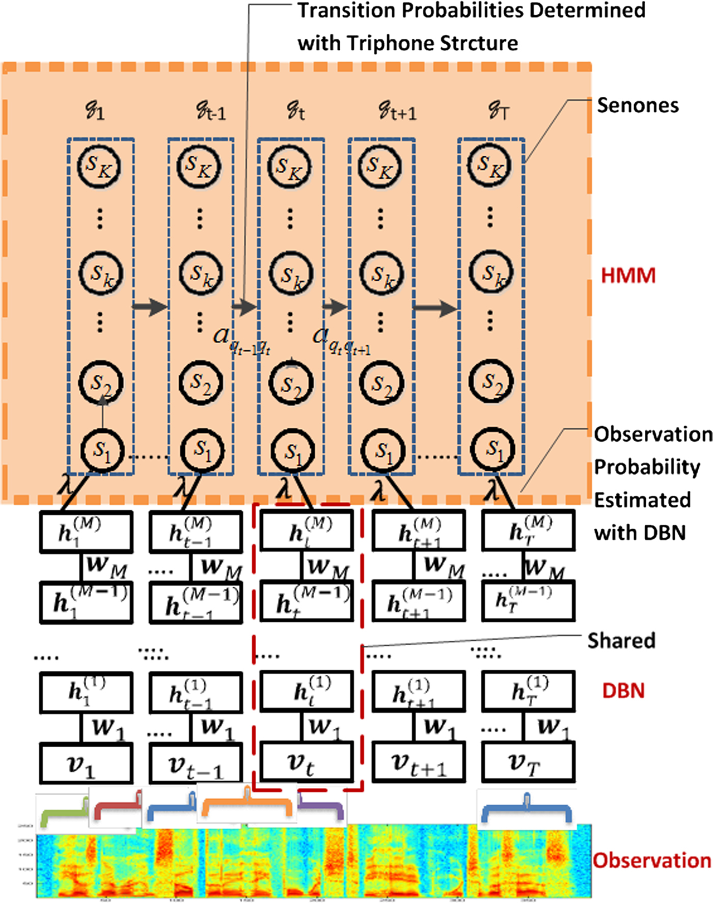
Fig. 6. Interface between DBN–DNN and HMM to form a DNN–HMM. This architecture has been successfully used in speech recognition experiments reported in [25].
It is important to note that the unique elasticity of temporal dynamic of speech as elaborated in [Reference Deng53] would require temporally-correlated models better than HMM for the ultimate success of speech recognition. Integrating such dynamic models having realistic co-articulatory properties with the DNN and possibly other deep learning models to form the coherent dynamic deep architecture is a challenging new research.
VI. DISCRIMINATIVE ARCHITECTURES: DSN AND RECURRENT NETWORK
A) Introduction
While the DNN just reviewed has been shown to be extremely powerful in connection with performing recognition and classification tasks including speech recognition and image classification, training a DBN has proven to be more difficult computationally. In particular, conventional techniques for training DNN at the fine tuning phase involve the utilization of a stochastic gradient descent learning algorithm, which is extremely difficult to parallelize across-machines. This makes learning at large scale practically impossible. For example, it has been possible to use one single, very powerful GPU machine to train DNN-based speech recognizers with dozens to a few hundreds of hours of speech training data with remarkable results. It is very difficult, however, to scale up this success with thousands or more hours of training data.
Here we describe a new deep learning architecture, DSN, which attacks the learning scalability problem. This section is based in part on the recent publications of [Reference Deng, Tur, He and Hakkani-Tur11, Reference Deng and Yu107, Reference Hutchinson, Deng and Yu111, Reference Hutchinson, Deng and Yu112] with expanded discussions.
The central idea of DSN design relates to the concept of stacking, as proposed originally in [Reference Wolpert159], where simple modules of functions or classifiers are composed first and then they are “stacked” on top of each other in order to learn complex functions or classifiers. Various ways of implementing stacking operations have been developed in the past, typically making use of supervised information in the simple modules. The new features for the stacked classifier at a higher level of the stacking architecture often come from concatenation of the classifier output of a lower module and the raw input features. In [Reference Cohen and de Carvalho160], the simple module used for stacking was a CRF. This type of deep architecture was further developed with hidden states added for successful natural language and speech recognition applications where segmentation information in unknown in the training data [Reference Yu, Wang and Deng96]. Convolutional neural networks, as in [Reference Jarrett, Kavukcuoglu and LeCun161], can also be considered as a stacking architecture but the supervision information is typically not used until in the final stacking module.
The DSN architecture was originally presented in [Reference Deng and Yu107], which also used the name Deep Convex Network or DCN to emphasize the convex nature of the main learning algorithm used for learning the network. The DSN discussed in this section makes use of supervision information for stacking each of the basic modules, which takes the simplified form of multi-layer perceptron. In the basic module, the output units are linear and the hidden units are sigmoidal non-linear. The linearity in the output units permits highly efficient, parallelizable, and closed-form estimation (a result of convex optimization) for the output network weights given the hidden units' activities. Owing to the closed-form constraints between the input and output weights, the input weights can also be elegantly estimated in an efficient, parallelizable, batch-mode manner.
The name “convex” used in [Reference Deng and Yu107] accentuates the role of convex optimization in learning the output network weights given the hidden units' activities in each basic module. It also points to the importance of the closed-form constraints, derived from the convexity, between the input and output weights. Such constraints make the learning the remaining network parameters (i.e., the input network weights) much easier than otherwise, enabling batch-mode learning of DSN that can be distributed over CPU clusters. And in more recent publications, DSN was used when the key operation of stacking is emphasized.
B) An architectural overview of DSN
A DSN, shown in Fig. 7, includes a variable number of layered modules, wherein each module is a specialized neural network consisting of a single hidden layer and two trainable sets of weights. In Fig. 7, only four such modules are illustrated, where each module is shown with a separate color. (In practice, up to a few hundreds of modules have been efficiently trained and used in image and speech classification experiments.)
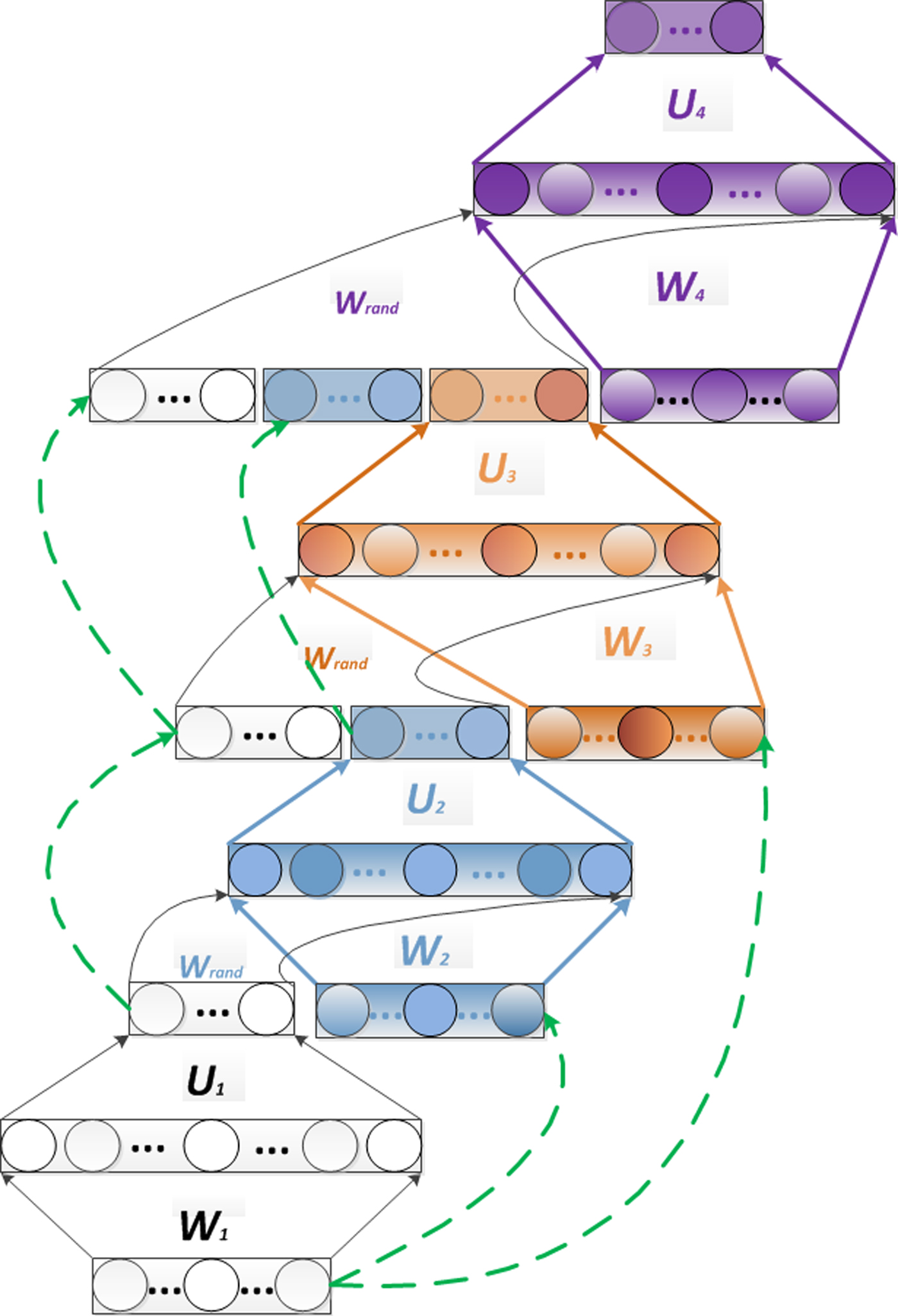
Fig. 7. A DSN architecture with input–output stacking. Only four modules are illustrated, each with a distinct color. Dashed lines denote copying layers.
The lowest module in the DSN comprises a first linear layer with a set of linear input units, a non-linear layer with a set of non-linear hidden units, and a second linear layer with a set of linear output units.
The hidden layer of the lowest module of a DSN comprises a set of non-linear units that are mapped to the input units by way of a first, lower-layer weight matrix, which we denote by W . For instance, the weight matrix may comprise a plurality of randomly generated values between zero and one, or the weights of an RBM trained separately. The non-linear units may be sigmoidal units that are configured to perform non-linear operations on weighted outputs from the input units (weighted in accordance with the first weight matrix W ).
The second, linear layer in any module of a DSN includes a set of output units that are representative of the targets of classification. The non-linear units in each module of the DSN may be mapped to a set of the linear output units by way of a second, upper-layer weight matrix, which we denote by U . This second weight matrix can be learned by way of a batch learning process, such that learning can be undertaken in parallel. Convex optimization can be employed in connection with learning U . For instance, U can be learned based at least in part upon the first weight matrix W , values of the coded classification targets, and values of the input units.
As indicated above, the DSN includes a set of serially connected, overlapping, and layered modules, wherein each module includes the aforementioned three layers – a first linear layer that includes a set of linear input units whose number equals the dimensionality of the input features, a hidden layer that comprises a set of non-linear units whose number is a tunable hyper-parameter, and a second linear layer that comprises a plurality of linear output units whose number equals that of the target classification classes. The modules are referred to herein as being layered because the output units of a lower module are a subset of the input units of an adjacent higher module in the DSN. More specifically, in a second module that is directly above the lowest module in the DSN, the input units can include the output units or hidden units of the lower module(s). The input units can additionally include the raw training data – in other words, the output units of the lowest module can be appended to the input units in the second module, such that the input units of the second module also include the output units of the lowest module.
The pattern discussed above of including output units in a lower module as a portion of the input units in an adjacent higher module in the DBN and thereafter learning a weight matrix that describes connection weights between hidden units and linear output units via convex optimization can continue for many modules. A resultant learned DSN may then be deployed in connection with an automatic classification task such as frame-level speech phone or state classification. Connecting DSNs output to an HMM or any dynamic programming device enables continuous speech recognition and other forms of sequential pattern recognition.
C) Learning DSN weights
Here, some technical detail is provided as to how the use of linear output units in DSN facilitates the learning of the DSN weights. A single module is used to illustrate the advantage for simplicity reasons. First, it is clear that the upper layer weight matrix U can be efficiently learned once the activity matrix H over all training samples in the hidden layer is known. Let us denote the training vectors by X = [ x 1, …, x i , …, x N ], in which each vector is denoted by x i = [x 1i , …, x ji , …, x Di ] T where D is the dimension of the input vector, which is a function of the block, and N is the total number of training samples. Denote by L the number of hidden units and by C the dimension of the output vector. Then, the output of a DSN block is y i = U T h i , where h i = σ ( W T x i ) is the hidden-layer vector for sample i, U is an L × C weight matrix at the upper layer of a block. W is a D × L weight matrix at the lower layer of a block, and σ (·) is a sigmoid function. Bias terms are implicitly represented in the above formulation if x i and h i are augmented with ones.
Given target vectors in the full training set with a total of N samples, T = [ t 1,…, t i ,…, t N ], where each vector is t i = [t 1i ,…,t ji ,…t Ci ] T , the parameters U and W are learned so as to minimize the average of the total square error below:
 $$E = {1 \over 2} \sum_n \Vert y_n - t_n \Vert^2 = {1\over2}{\rm Tr} \lsqb \lpar {\bf Y}-{\bf T}\rpar \lpar {\bf Y}-{\bf T}\rpar ^{\rm T}\rsqb \comma \;$$
where the output of the network is
 $${\bi y}_n = {\bi U}^T {\bi h}_n = {\bi U}^T\sigma \lpar {\bi W}^T {\bi x}_n\rpar = G_n \lpar {\bi U}\comma \; {\bi W}\rpar$$
which depends on both weight matrices, as in the standard neural net. Assuming H = [ h 1,…, h i ,…, h N ] is known, or equivalently, W is known. Then, setting the error derivative with respective to U to zero gives
 $${\bi U} = \lpar \bi HH^T\rpar ^{-1} {\bi HT}^T = {\rm F}\lpar \bi W\rpar \comma \; \quad {\rm where}\quad {\bi h}_n = \sigma \lpar {\bi W}^T {\bi x}_n\rpar$$
This provides an explicit constraint between U , and W , which were treated independently in the popular backprop algorithm.
Now, given the equality constraint U = F( W ), let us use the Lagrangian multiplier method to solve the optimization problem in learning W . Optimizing the Lagrangian:
 $$E = {1 \over 2} \sum_n \Vert G_n \lpar \bi U\comma \; \bi W\rpar - {\bi t}_n \Vert^2 + \lambda \Vert {\bi U} - {\rm F}\lpar W\rpar \Vert\comma \;$$
we can derive batch-mode gradient descent learning algorithm where the gradient takes the following form [Reference Deng, Yu and Platt108]:
 $$\eqalign{{\partial E \over \partial {\bi W}} & = 2{\bi X} \left[{\bi H}^T \circ \lpar 1- {\bi H}\rpar ^T \circ \left[{\bi H}^{\dagger} \lpar {\bi HT}^T\rpar \lpar {\bi TH}^\dagger\rpar \right.\right. \cr & \left.\left. \quad - {\bi T}^T \lpar {\bi TH}^\dagger\rpar \right]\right]}$$
where H † = H T ( HH T )−1 is pseudo-inverse of H and symbol ○ denotes component-wise multiplication.
Compared with backprop, the above method has less noise in gradient computation due to the exploitation of the explicit constraint U = F( W ). As such, it was found experimentally that, unlike backprop, batch training is effective, which aids parallel learning of DSN.
D) Tensorized DSN
The DSN architecture discussed so far has recently been generalized to its tensorized version, which we call TDSN [Reference Hutchinson, Deng and Yu111, Reference Hutchinson, Deng and Yu112]. It has the same scalability as DSN in terms of parallelizability in learning, but it generalizes DSN by providing higher-order feature interactions missing in DSN.
The architecture of TDSN is similar to that of DSN in the way that stacking operation is carried out. That is, modules of the TDSN are stacking up in a similar way to form a deep architecture. The differences of TDSN and DSN lie mainly in how each module is constructed. In DSN, we have one set of hidden units forming a hidden layer, as denoted at the left panel of Fig. 8. In contrast, each module of a TDSD contains two independent hidden layers, denoted as “Hidden 1” and “Hidden 2” in the middle and right panels of Fig. 8. As a result of this different, the upper-layer weights, denoted by “U” in Fig. 8, changes from a matrix (a two-dimensional array) in DSN to a tensor (a three-dimensional array) in TDSN, shown as a cube labeled by “U” in the middle panel.
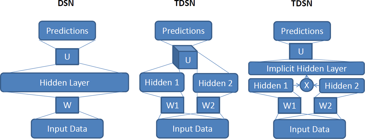
Fig. 8. Comparisons of one single module of a DSN (left) and that of a tensorized-DSN (TDSN). Two equivalent forms of a TDSN module are shown to the right.
The tensor U has a three-way connection, one to the prediction layer and the remaining to the two separate hidden layers. An equivalent form of this TDSN module is shown in the right panel of Fig. 8, where the implicit hidden layer is formed by expanding the two separate hidden layers into their outer product. The resulting large vector contains all possible pair-wise products for the two sets of hidden-layer vectors. This turns tensor U into a matrix again whose dimensions are (1) size of the prediction layer; and (2) product of the two hidden layers' sizes. Such equivalence enables the same convex optimization for learning U developed for DSN to be applied to learning tensor U. Importantly, higher-order hidden feature interactions are enabled in TDSN via the outer product construction for the large, implicit hidden layer.
Stacking TDSN modules to form a deep architecture pursues in a similar way to DSN by concatenating various vectors. Two examples are shown in Figs 9 and 10. Note stacking by concatenating hidden layers with input (Fig. 10) would be difficult for DSN since its hidden layer tends to be too large for practical purposes.
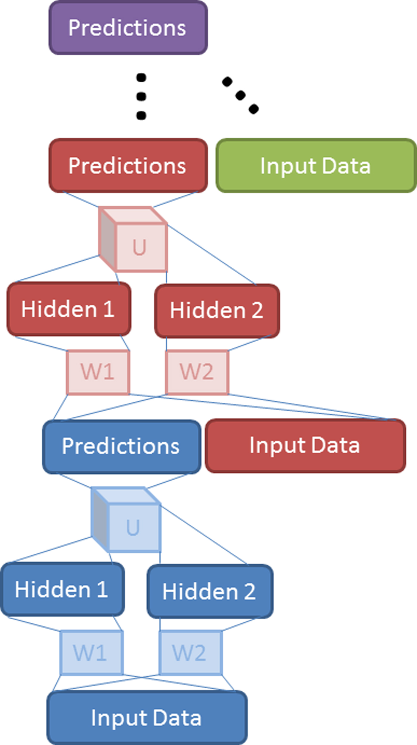
Fig. 9. Stacking of TDSN modules by concatenating prediction vector with input vector.
Fig. 10. Stacking of TDSN modules by concatenating two hidden-layers' vectors with the input vector.
E) Recurrent neural networks
If we consider the increasingly higher modules of a DSN as time-shifted versions of a “shallow” neural network, then we can turn a DSN (with input-hidden stacking instead of input-output stacking) into a temporally-RNN, where the discrete time index corresponds to the depth in the DSN. The constraints in the DSN among weight matrices can be similarly applied to this type of RNN in learning its weight parameters, provided that the output units are linear. (In fact, the concepts of RNN and DSN can be combined to form a recurrent version of the DSN, or equivalently, a stacked version of a simple RNN, which will not be discussed in this paper).
One way of learning the RNNs with linear outputs is to adopt the approach shown to be effective for DSN learning outlined in Section VI-C above. This would capture a short memory of one time step. To increase the memory length, we can apply the traditional method of Backprop through time (BPTT) but exploit the relationship among various weight matrices to turn the recursive procedure to a simpler analytical form. However, this is more difficult to formulate and derive than for the DSN case discussed in Section VI-C. The use of the general BPTT [Reference Pascanu, Mikolov and Bengio162] has the advantage of handling non-linear output units, shown to speed up learning substantially compared with the use of linear output units in an RNN. The commonly discussed problem of vanishing or exploding gradients in BPTT can be mitigated by applying constraints regarding the RNN's recurrent matrices during the optimization process.
In the remainder of this section, let us formulate the RNN in terms of the non-linear state space model commonly used in signal processing. I will compare it with the same state-space formulation of non-linear dynamic systems used as generative models for speech acoustics. The contrast between the discriminative RNN and the use of the same mathematical model in the generative mode allows us to shed light onto why one approach works better than another.
In the RNN, the state dynamic (noise free) is expressed as
 $${\bi h}_t = f\lpar {\bi W}_{xh} {\bi x}_t + {\bi W}_{hh} {\bi h}_{t-1}\rpar .$$
The “observation” is the predicted “labels” or target vector, l t , a vector of one-hot coded class labels. The “observation equation” in the state-space formulation becomes [Reference Graves, Mahamed and Hinton116]:
 $$y_t = {\bi W}_{hy} {\bi h}_t \quad \hbox{or}\quad {\bi y}_t = g\lpar {\bi W}_{hy} {\bi h}_t\rpar .$$
Define the error function as a sum of squared differences between y t and l t over time, or cross-entropy between them. Then BPTT unfolds the RNN over time in computing the gradients with respect to W hy , W xh , and W hh , and stochastic gradient descent is applied to update these weight matrices.
Using a similar state-space formulation of the RNN model above but in a generative mode, known as the hidden dynamic model as briefly discussed in Section III-A, speech recognition researchers have built many types of speech recognizers over the past 20 some years; see a survey in Sections III-D and III-E of [Reference Deng and Li34]. In particular, the corresponding state and observation equations in the generative are
 $$\eqalign{{\bi h}_t & = G\lpar {\bi h}_{t-1} + \Lambda_{l_t}\rpar + \hbox{State Noise} \cr \quad x_{t} &= H\lpar {\bi h}_t\comma \; \Omega_{l_t}\rpar + \hbox{ObsNoise}}$$
[Rewritten from equations (13) and (14) in [Reference Deng and Li34] to be consistent with the RNN variables]. Here, Λ l t is the system matrix driving the (articulatory-like) state dynamics, which is dependent on the label l t at time t, hence the model is also called a switching dynamic system. These system matrix parameters are analogous to W hh in the RNN. Ω l t is the parameter set that governs the non-linear mapping from the hidden (articulatory-like) states in speech production to acoustic features of speech. In one implementation, Ω l t took the form of shallow MLP weights [Reference Picone69, Reference Deng and Ma163, Reference Togneri and Deng164]. In another implementation, Ω l t took the form of a set of matrices in a mixture of linear experts [Reference Ma and Deng73].
The state equation in many existing implementations of the hidden dynamic models of speech does not take non-linear forms. Rather, the following linear form was used (e.g., [Reference Deng and Ma163]):
 $${\bi h}_t = {\bi W}_{hh} \lpar l_t\rpar {\bi h}_{t-1} + \lsqb {\bi I} - {\bi W}_{hh} \lpar l_t\rpar \rsqb {\bi t} \lpar l_t\rpar + \hbox{State Noise}$$
which exhibits the target-directed property for the articulatory-like dynamics. Here, the parameters W hh is a function of the (phonetic) label l t at a particular time t, and t (l t ) is a mapping between the symbolic quantity l t to a continuous-valued “target” vector.
On the surface and based on the mathematical description, there are striking similarities between the discriminative RNN and generative hidden dynamic model. However, the essence as well as the representational substance of the two models are very different, which we summarize below.
First, the RNN adopts the strategy of using distributed representations for the supervision information (i.e., labels), whereas in the hidden dynamic model, the labels are locally represented and used to index separate sets of time-varying parameters Λ l t and Ω l t leading to “switching” dynamics, which considerably complicates the decoding computation. Second, the RNN runs “bottom-up”, directly producing posterior probabilities of all classes. In contrast, the hidden dynamic model runs “top down”, generating likelihood values for each class individually. This difference is most clear by comparing the two observations equations, one gives label prediction and another gives input feature prediction. In the state equations, the RNN model has the input to drive the system dynamics, whereas the generative model has the label index to drive the dynamics (via an intermediate representation of articulatory or vocal tract resonance “targets”). Third, the learning algorithms of BPTT for the RNN directly minimize the label prediction errors. In contrast, non-linear Kalman filtering (E step of the EM algorithm) used for learning the generative model does not do discrimination explicitly. Given the known difficulties of BPTT for RNN [Reference Pascanu, Mikolov and Bengio162], one obvious direction is to adopt the hybrid deep architecture by using the generative hidden dynamic model to pretrain the discriminative RNN, analogous to using the generative DBN to pretrain the DNN discussed in the preceding subsection.
VII. APPLICATIONS OF DEEP LEARNING TO SIGNAL AND INFORMATION PROCESSING
In the expanded technical scope of signal processing, the signal is endowed with not only the traditional types such as audio, speech, image and video, but also text, language, and document that convey high-level, semantic information for human consumption. In addition, the scope of processing has been extended from the conventional coding, enhancement, analysis, and recognition to include more human-centric tasks of interpretation, understanding, retrieval, mining, and user interface [Reference Deng2]. Signal processing researchers have been working on one or more of the signal processing areas defined by the matrix constructed with the two axes of signal and processing discussed here. The deep learning techniques discussed in this paper have recently been applied to a large number of traditional and extended signal-processing areas, with some recent interesting application of predicting protein structure [Reference Lena, Nagata and Baldi110], which we will not cover here. We now provide a brief survey of this body of work in four main categories pertaining closely to signal and information processing.
A) Speech and audio
The traditional neural network or MLP has been in use for speech recognition for many years. When used alone, its performance is typically lower than the state-of-the-art HMM systems with observation probabilities approximated with GMMs. Recently, the deep learning technique was successfully applied to phone recognition [Reference Mohamed, Yu and Deng23, Reference Mohamed, Dahl and Hinton24, Reference Graves, Mahamed and Hinton116, Reference Deng, Abdel-Hamid and Yu126, Reference Mohamed, Dahl and Hinton165, Reference Sivaram and Hermansky166] and large vocabulary speech recognition tasks [Reference Dahl, Yu, Deng and Acero22, Reference Dahl, Yu, Deng and Acero25, Reference Yu, Seide, Li and Deng135, Reference Seide, Li and Yu155, Reference Yan, Huo and Xu156, Reference Kubo, Hori and Nakamura167–Reference Deng, Hinton and Kingsbury169] by integrating the powerful discriminative training ability of DNNs with the sequential modeling ability of HMMs.
Speech recognition has long been dominated by the GMM–HMM method, with an underlying shallow generative model [Reference Waibel, Hanazawa, Hinton, Shikano and Lang129, Reference Juang, Levinson and Sondhi170, Reference Deng, Lennig, Seitz and Mermelstein171]. Neural networks once were a popular approach but had not been competitive with the GMM–HMM [Reference Bourlard and Morgan32, Reference Morgan33, Reference Deng, Hassanein and Elmasry113, Reference Waibel, Hanazawa, Hinton, Shikano and Lang129]. Generative models with deep hidden dynamics likewise have not been competitive either [Reference Picone69, Reference Deng, Yu and Acero74]. Deep learning and DNN started making impact in speech recognition in 2010, after close collaborations between academic and industrial researchers (see reviews in [Reference Hinton6, Reference Deng, Hinton and Kingsbury169]. The collaborative work started in small vocabulary tasks [Reference Mohamed, Yu and Deng23, Reference Mohamed, Dahl and Hinton24, Reference Deng, Seltzer, Yu, Acero, Mohamed and Hinton30, Reference Deng, Abdel-Hamid and Yu126, Reference Mohamed, Dahl and Hinton165], demonstrating the power of hybrid deep architectures. The work also showed the importance of raw speech features of spectrogram – back from the long-popular MFCC features, but not yet reaching the raw speech-waveform level [Reference Sheikhzadeh and Deng173, Reference Jaitly and Hinton174]. The collaboration continued to large vocabulary tasks with more convincing, highly positive results [Reference Dahl, Yu, Deng and Acero22, Reference Dahl, Yu, Deng and Acero25, Reference Yu, Wang, Karam and Deng103]. This success is in large part attributed to the use of a very large DNN output layer structured in the same way as the GMM–HMM speech units (senones), motivated initially by the speech industry's desire to keep the change of the already highly efficient decoder software's infrastructure to a minimum. In the meantime, this body of work also demonstrated the possibility to reduce the need for the DBN-like pretraining in effective learning of DNNs when a large amount of labeled data is available. A combination of three factors quickly spread the success of deep learning in speech recognition to the entire speech industry and academia: (1) minimally required decoder changes under the new DNN-based speech recognizer deployment conditions enabled by the use of senones as the DNN output; (2) significantly lowered errors compared with the then-state-of-the-art GMM-HMM system; and (3) training simplicity empowered by big data for training. By the ICASSP-2013 timeframe, at least 15 major speech recognition groups worldwide confirmed the experimental success of DNNs with very large tasks and with the use of raw speech spectral features away from MFCCs. The most notable groups include all major industrial speech labs worldwide: Microsoft [Reference Seide, Li and Yu155, Reference Yan, Huo and Xu156, Reference Deng168, Reference Deng, Hinton and Kingsbury169], IBM [Reference Sainath, Mohamed, Kingsbury and Ramabhadran125, Reference Kingsbury, Sainath and Soltau141, Reference Sainath, Kingbury, Ramabhadran, Novak and Mohamed175], Google [Reference Dean120, Reference Jaitly, Nguyen and Vanhoucke176], and Baidu. Their results represent a new state-of-the-art in speech recognition widely deployed in these companies' voice products and services with extensive media coverage.
As discussed in Section III-B, the concept of convolution in time was originated in TDNN as a shallow neural net [Reference Lang, Waibel and Hinton127, Reference Waibel, Hanazawa, Hinton, Shikano and Lang129] developed in early speech recognition. Only recently and when deep architectures (e.g., deep CNN) are used, it has been found that frequency-dimension weight sharing is more effective for high-performance phone recognition than time domain as in the previous TDNN [Reference Abdel-Hamid, Mohamed, Jiang and Penn122–Reference Abdel-Hamid, Deng, Yu and Jiang124, Reference Deng, Abdel-Hamid and Yu126]. These studies also show that designing the pooling in deep CNN to properly trade-off between invariance to vocal tract length and discrimination between speech sounds (together with a regularization technique of “dropout” [Reference Hinton, Srivastava, Krizhevsky, Sutskever and Salakhutdinov177] leads to even better phone recognition performance. This set of work also points to the direction of trading-off between trajectory discrimination and invariance expressed in the whole dynamic pattern of speech defined in mixed time and frequency domains using convolution and pooling. Moreover, the most recent work of [Reference Sainath, Mohamed, Kingsbury and Ramabhadran125] shows that CNNs are also useful for large vocabulary continuous speech recognition and further demonstrates that multiple convolutional layers provide even more improvement when the convolutional layers use a large number of convolution kernels or feature maps.
In addition to the RBM, DBN, CNN, and DSN, other deep models have also been developed and reported in the literature for speech and audio processing and related applications. For example, the deep-structured CRF, which stacks many layers of CRFs, have been successfully used in the task of language identification [Reference Yu, Wang, Karam and Deng103], phone recognition [Reference Yu and Deng102], sequential labeling in natural language processing [Reference Yu, Wang and Deng96], and confidence calibration in speech recognition [Reference Yu, Deng and Dahl178, Reference Yu, Li and Deng179]. Furthermore, while RNN has early success in phone recognition [Reference Robinson114], it was not easy to duplicate due to the intricacy in training, let alone to scale up for larger speech recognition tasks. Learning algorithms for RNNs have been dramatically improved since then, and better results have been obtained recently using RNNs [Reference Graves, Fernandez, Gomez and Schmidhuber115, Reference Maas, Le, O'Neil, Vinyals, Nguyen and Ng180], especially when the structure of long short-term memory (LSTM) is embedded into the RNN with several layers and trained bi-directionally [Reference Graves, Mahamed and Hinton116] RNNs have also been recently applied to audio/music processing applications [Reference Bengio, Boulanger and Pascanu49], where the use of rectified linear hidden units instead of logistic or tanh non-linearities is explored in RNN. Rectified linear units (ReLU) compute y = max(x, 0), and lead to sparser gradients, less diffusion of credit and blame in the RNN, and faster training.
In addition to speech recognition, the impact of deep learning has recently spread to speech synthesis, aimed to overcome the limitations of the conventional approach in statistical parametric synthesis based on Gaussian-HMM and decision-tree-based model clustering. At conference ICASSP (May, 2013), four different deep learning approaches are reported to improve the traditional HMM-based speech synthesis systems. In Ling et al. [Reference Ling, Richmond and Yamagishi64, Reference Ling, Deng and Yu181], the RBM and DBN as generative models are used to replace the traditional Gaussian models, achieving significant quality improvement, in both subjective and objective measures, of the synthesized voice. In the approach developed in [Reference Kang, Qian and Meng182], the DBN as a generative model is used to represent joint distribution of linguistic and acoustic features. Both the decision trees and Gaussian models are replaced by the DBN. On the other hand, the study reported in [Reference Zen, Senior and Schuster183] makes use of the discriminative model of the DNN to represent the conditional distribution of the acoustic features given the linguistic features. No joint distributions are modeled. Finally, in [Reference Fernandez, Rendel, Ramabhadran and Hoory184], the discriminative model of DNN is used as a feature extractor that summarizes high-level structure from the raw acoustic features. Such DNN features are then used as the input for the second stage of the system for the prediction of prosodic contour targets from contextual features in the fill speech synthesis system. The application of deep learning to speech synthesis is in its infancy, and much more work is expected from that community in the near future.
Likewise, in audio and music processing, deep learning has also become of intense interest only recently. The impacted areas include mainly music signal processing and music information retrieval [Reference Bengio, Boulanger and Pascanu49, Reference Humphrey, Bello and LeCun185–Reference Schmidt and Kim187]. Deep learning presents a unique set of challenges in these areas. Music audio signals are time series where events are organized in musical time, rather than in real time, which changes as a function of rhythm and expression. The measured signals typically combine multiple voices that are synchronized in time and overlapping in frequency, mixing both short-term and long-term temporal dependencies. The influencing factors include musical tradition, style, composer and interpretation. The high complexity and variety give rise to the signal representation problems well-suited to the high levels of abstraction afforded by the perceptually and biologically motivated processing techniques of deep learning. Again, much more work is expected from the music and audio signal processing community in the near future.
B) Image, video, and multimodality
The original DBN and deep autoencoder were developed and demonstrated with success on the simple image recognition and dimensionality reduction (coding) tasks (MNIST) in [Reference Hinton and Salakhutdinov21]. It is interesting to note that the gain of coding efficiency using the DBN-based autoencoder on the image data over the conventional method of principal component analysis as demonstrated in [Reference Hinton and Salakhutdinov21] is very similar to the gain reported in [Reference Deng, Seltzer, Yu, Acero, Mohamed and Hinton30] on the speech data over the traditional technique of VQ.
In [Reference Nair and Hinton188], a modified DBN is developed where the top-layer model uses a third-order BM. This type of DBN is applied to the NORB database – a three-dimensional object recognition task. An error rate close to the best published result on this task is reported. In particular, it is shown that the DBN substantially outperforms shallow models such as SVMs.
Deep architectures with convolution structure have been found highly effective and been commonly used in computer vision and image recognition [Reference LeCun, Bottou, Bengio and Haffner118–Reference Krizhevsky, Sutskever and Hinton121, Reference Le, Ranzato, Monga, Devin, Corrado, Chen, Dean and Ng154, Reference Jarrett, Kavukcuoglu and LeCun161, Reference LeCun, Bengio and Arbib189, Reference Kavukcuoglu, Sermanet, Boureau, Gregor, Mathieu and LeCun190]. The most notable advance was recently achieved in the 2012 ImageNet LSVRC contest, where 1000 different image classes are the targets with 1.2 million high-resolution images in the training set. On the test set consisting of 150 000 images, the deep CNN approach described in [Reference Krizhevsky, Sutskever and Hinton121] achieved the error rates considerably lower than the previous state-of-the-art. Very large deep CNNs are used, consisting of 60 million weights, and 650 000 neurons, and five convolutional layers together with max-pooling layers. Additional three fully-connected layers as in the DNN described previously are used on top of the deep CNN layers. Although all the above structures were developed separately in earlier work, their best combination accounted for part of the success. Additional factors contributing to the final success are: (1) a powerful regularization technique called “dropout” (see details in [Reference Hinton, Srivastava, Krizhevsky, Sutskever and Salakhutdinov177]; and (2) use of non-saturating neurons or ReLU that compute y = max(x, 0), significantly speeding up the training process especially with a very efficient GPU implementation. More recently, a similar deep CNN approach with stochastic pooling also reported excellent results in four image datasets [Reference Zeiler and Fergus191]. Deep networks are shown to be powerful for computer vision and image recognition tasks because they extract appropriate features while jointly performing discrimination [Reference LeCun192].
In another type of deep architecture that has created substantial impact in image recognition, Le et al. [Reference Le, Ranzato, Monga, Devin, Corrado, Chen, Dean and Ng154] reported excellent results using a generative model based on sparse autoencoders in a largely un-supervised framework. This type of extremely large networks (11 billion parameters) was trained using thousands of CPU cores. The most recent work along this direction reported that of the same size of the network can be alternatively trained using a cluster of only 16 GPU server machines [Reference Coates, Huval, Wang, Wu, Ng and Catanzaro193].
The use of a temporally conditional DBN for video sequence and human motion synthesis is reported in [Reference Taylor, Hinton and Roweis85]. The conditional DBN makes the DBN weights associated with a fixed time window conditioned on the data from previous time steps. The computational tool offered in this type of temporal DBN and the related recurrent networks may provide the opportunity to improve the DBN–HMMs toward efficient integration of temporal-centric human speech production mechanisms into DBN-based speech production model.
An interesting study appeared in [Reference Ngiam, Khosla, Kim, Nam, Lee and Ng37, Reference Ngiam, Chen, Koh and Ng38], where the authors propose and evaluate a novel application of deep networks to learn features over both audio and video modalities. A similar deep autoencoder architecture described in Section IV and in [Reference Deng, Seltzer, Yu, Acero, Mohamed and Hinton30] is used but it can be considered as a generalization from a single modality to two modalities. Cross-modality feature learning has been demonstrated – better features for video can be learned if both audio and video information sources are available at feature learning time. The authors further show how to learn a shared audio and video representation, and evaluate it on a fixed task, where the classifier is trained with audio-only data but tested with video-only data and vice versa. The work concludes that deep learning architectures are generally effective in learning multimodal features from unlabeled data and in improving single modality features through cross-modality learning. One exception is the cross-modality setting using the CUAVE dataset. The results presented in [Reference Ngiam, Khosla, Kim, Nam, Lee and Ng37, Reference Ngiam, Chen, Koh and Ng38] show that there is an improvement by learning video features with both video and audio compared to learning features with only video data. However, the same paper also shows that a model of [Reference Papandreou, Katsamanis, Pitsikalis and Maragos194] in which a sophisticated signal processing technique for extracting visual features, together with the uncertainty-compensation method developed originally from robust speech recognition [Reference Deng, Wu, Droppo and Acero195], gives the best classification accuracy in the cross-modeling learning task, beating the features derived from the generative deep architecture designed for this task.
While the deep generative architecture for multimodal learning described in [Reference Ngiam, Khosla, Kim, Nam, Lee and Ng37, Reference Ngiam, Chen, Koh and Ng38] is based on non-probabilistic autoencoder neural nets, a probabilistic version based on DBM has appeared more recently for the same multimodal application. In [Reference Srivastava and Salakhutdinov42], a DBM is used to extract a unified representation integrating separate modalities, useful for both classification and information retrieval tasks. Rather than using the “bottleneck” layers in the deep autoencoder to represent multimodal inputs, here a probability density is defined on the joint space of multimodal inputs, and states of suitably defined latent variables are used for the representation. The advantage of this probabilistic formulation, lacking in the deep autoencoder, is that the missing modality's information can be filled in naturally by sampling from its conditional distribution. For the bimodal data consisting of image and text, the multimodal DBM is shown to outperform deep multimodal autoencoder as well as multimodal DBN in classification and information retrieval tasks.
C) Language modeling
Research in language, document, and text processing has seen increasing popularity recently in the signal processing community, and has been designated as one of the main focus areas by the society's audio, speech, and language processing technical committee. There has been a long history (e.g., [Reference Bengio, Ducharme, Vincent and Jauvin196, Reference Zamora-Martínez, Castro-Bleda and España-Boquera197]) of using (shallow) neural networks in LM – an important component in speech recognition, machine translation, text information retrieval, and in natural language processing. Recently, DNNs have been attracting more and more attention in statistical LM.
An LM is a function that captures the salient statistical characteristics of the distribution of sequences of words in a natural language. It allows one to make probabilistic predictions of the next word given preceding ones. A neural network LM is one that exploits the neural network ability to learn distributed representations to reduce the impact of the curse of dimensionality.
A distributed representation of a symbol is a vector of features which characterize the meaning of the symbol. With a neural network LM, one relies on the learning algorithm to discover meaningful, continuous-valued features. The basic idea is to learn to associate each word in the dictionary with a continuous-valued vector representation, where each word corresponds to a point in a feature space. One can imagine that each dimension of that space corresponds to a semantic or grammatical characteristic of words. The hope is that functionally similar words get to be closer to each other in that space, at least along some directions. A sequence of words can thus be transformed into a sequence of these learned feature vectors. The neural network learns to map that sequence of feature vectors to the probability distribution over the next word in the sequence.
The distributed representation approach to LM has the advantage that it allows the model to generalize well to sequences that are not in the set of training word sequences, but that are similar in terms of their features, i.e., their distributed representation. Because neural networks tend to map nearby inputs to nearby outputs, the predictions corresponding to word sequences with similar features are mapped to similar predictions.
The above ideas of neural network LM have been implemented in various studies, some involving deep architecture. In [Reference Mnih and Hinton198], temporally factored RBM was used for LM. Unlike the traditional N-gram model the factored RBM uses distributed representations not only for context words but also for the words being predicted. This approach is generalized to deeper structures as reported in [Reference Mnih and Hinton199].
More recent work on neural network LM with deep architectures can be found in [Reference Mikolov, Karafiat, Burget, Cernocky and Khudanpur51, Reference Le, Allauzen, Wisniewski and Yvon200–Reference Mikolov203]. In particular, the work described in [Reference Mikolov, Deoras, Povey, Burget and Cernocky202, Reference Mikolov203] makes use RNNs to build large scale language models. It achieves stability and fast convergence in training, helped by capping the growing gradient in training RNNs. It also develops adaptation schemes for the RNN-based LM by sorting the training data with respect to their relevance and by training the model during processing of the test data. Empirical comparisons with other LM state-of-the-art show much better performance of RNN especially in the perplexity measure. A separate work on applying RNN as an LM on the unit of characters instead of words can be found in [Reference Sutskever, Martens and Hinton46]. Very interesting properties such as predicting long-term dependency (e.g., making open and closing quotes in a paragraph) are demonstrated. But its usefulness in practical applications has not been clear because word is such a powerful representation for natural language and changing word to character in LM limits most practical application scenarios.
Furthermore, the use of hierarchical Bayesian priors in building up deep and recursive structure in LM appeared in [Reference Huang and Renals204]. Specifically, Pitman–Yor process is exploited as the Bayesian prior, from which a deep (four layers) probabilistic generative model is built. It offers a principled approach to LM smoothing by incorporating the power-law distribution for natural language. As discussed in Section III, this type of prior knowledge embedding is more readily achievable in the probabilistic modeling setup than in the neural network one.
D) Natural language processing
In the well-known and sometimes debatable work on natural language processing, Collobert and Weston [Reference Collobert and Weston205] developed and employed a convolutional DBN as the common model to simultaneously solve a number of classic problems including part-of-speech tagging, chunking, named entity tagging, semantic role identification, and similar word identification. More recent work reported in [Reference Collobert206] further developed a fast purely discriminative approach for parsing based on the deep recurrent convolutional architecture called Graph Transformer Network. Collobert et al. [Reference Collobert, Weston, Bottou, Karlen, Kavukcuoglu and Kuksa207] provides a comprehensive review on this line of work, specifically on ways of applying a unified neural network architectures and related deep learning algorithms to solve natural language processing problems from “scratch”. The theme of this line of work is to avoid task-specific, “man-made” feature engineering while providing versatility and unified features constructed automatically from deep learning applicable to all natural language-processing tasks. The system described in [Reference Collobert, Weston, Bottou, Karlen, Kavukcuoglu and Kuksa207] automatically learns internal representation from vast amounts of mostly unlabeled training data.
One most important aspect of the work described in [Reference Collobert and Weston205, Reference Collobert, Weston, Bottou, Karlen, Kavukcuoglu and Kuksa207] is the transformation of raw word representations in terms of sparse vectors with a very high dimension (vocabulary size or its square or even its cubic) into low-dimensional, real-valued vectors for processing by subsequent neural network layers. This is known as “word embedding”, widely used in natural language processing and LM nowadays. Unsupervised learning is used where “context” of the word is used as the learning signal in neural networks. An excellent tutorial was recently given [Reference Socher, Bengio and Manning208] that explains how the neural network is trained to perform word embedding originally proposed in [Reference Collobert and Weston205]. More recent work proposes new ways of doing word embedding that better capture the semantics of words by incorporating both local and global document context and better account for homonymy and polysemy by learning multiple embeddings per word [Reference Huang, Socher, Manning and Ng209]. Also, there is evidence that the use of RNN can also provide empirically good performance in word embedding [Reference Mikolov203].
The concept of word embedding was very recently extended from a single language to two, producing bilingual word embeddings for machine translation applications [Reference Zou, Socher, Cer and Manning210, Reference Gao, He, Yih and Deng211]. Good performance was shown by Zou et al. [Reference Zou, Socher, Cer and Manning210] on Chinese semantic similarity with bilingual trained embeddings. Use of such embeddings to compute semantic similarity of phrase pairs was shown to improve the BLEU score slightly in Chinese–English machine translation. On the other hand, Gao et al. [Reference Gao, He, Yih and Deng211] made use word embeddings in both source and target languages as the “raw” input features in DNNs to extract higher-level, semantic features. Then the translation score is computed by measuring the distance between the semantic features in the new feature space. The DNN weights are learned so as to directly optimize the quality of end-to-end BLEU score in machine translation.
Another area of applying deep learning to natural language processing appeared in [Reference Socher, Lin, Ng and Manning86], where a recursive neural network is used to build a deep, tree-like architecture. The network is shown to be capable of successful merging of natural language words based on the learned semantic transformations of their original features. This deep learning approach provides an excellent performance on natural language parsing. The same approach is also demonstrated by the same authors to be successful in parsing natural scene images. In related studies, a similar recursive deep architecture is used for paraphrase detection [Reference Socher, Pennington, Huang, Ng and Manning212], and for predicting sentiment distributions from text [Reference Socher, Pennington, Huang, Ng and Manning213]. In the most recent work, Socher et al. [Reference Socher, Perelygin, Wu, Chuang, Manning, Ng and Potts214] extended the recursive neural network to its tensor, in a similar way that the DNN was extended to its tensor version [Reference Yu, Deng and Seide215], and applied it to semantic compositionality. This recursive neural tensor network resulted in semantic word space capable of expressing the meaning of longer phrases, and drastically improved the prediction accuracy of sentiment labels.
E) Information retrieval
Here we discuss applications of the DBN, the related deep autoencoder, and more advanced deep learning methods developed more recently to document indexing and information retrieval.
Salakhutdinov and Hinton [Reference Salakhutdinov and Hinton216, Reference Hinton and Salakhutdinov217] showed that the hidden variables in the final layer of a DBN not only are easy to infer but also give a better representation of each document, based on the word-count features, than the widely used latent semantic analysis and the traditional TF-IDF approach for information retrieval. With the use of compact codes produced by a deep autoencoder, documents are mapped to memory addresses in such a way that semantically similar text documents are located at nearby address to facilitate rapid document retrieval. And the mapping from a word-count vector to its compact code is highly efficient, requiring only a matrix multiplication and a subsequent sigmoid function evaluation for each hidden layer in the encoder part of the network.
Briefly, the lowest layer of the DBN represents the word-count vector of a document and the top layer represents a leaned binary code for that document. The top two layers of the DBN form an undirected associative memory and the remaining layers form a Bayesian (also called belief) network with directed, top-down connections. This DBN, composed of a set of stacked RBMs as we reviewed in Section V, produces a feedforward “encoder” network that converts word-count vectors to compact codes. By composing the RBMs in the opposite order, a “decoder” network is constructed that maps compact code vectors into reconstructed word-count vectors. Combining the encoder and decoder, one obtains a deep autoencoder (subject to further fine-tuning as discussed in Section IV) for document coding and subsequent retrieval.
After the deep model is trained, the retrieval process starts with mapping each query document into a 128-bit binary code by performing a forward pass through the model with thresholding. Then, the similarity, with Hamming distance, between the query binary code and all other documents' 128-bit binary codes are computed efficiently.
While the “semantic hashing” method described above is intended to extract hierarchical semantic structure embedded in the query and the document, it nevertheless adopts an unsupervised learning approach where the DBN and deep autoencoder parameters are optimized for the reconstruction of the documents rather than for the real goal of information retrieval; i.e., to differentiate the relevant documents from the irrelevant ones for a given query. As a result, it fails to significantly outperform the baseline retrieval models based on keyword matching. Moreover, the semantic hashing model also faces the scalability challenge regarding large-scale matrix multiplication. Both of these problems are very recently addressed by Huang et al. [Reference Huang, He, Gao, Deng, Acero and Heck218], where a weakly supervised approach is taken. Specifically, in a series of deep structured semantic models (DSSM) developed in this work, deterministic word hashing is constructed from the documents and queries first, which produces vectors with relatively low dimensionality to feed to DNNs for extracting semantic features from the document-query pairs. In learning the DNNs, instead of using a cross-entropy as the optimization criterion, the DSSM constructs a novel objective function that directly targets the goal of document ranking, enabled by the availability of click-through data as the “supervision” information. This objective function is defined on the basis of the cosine similarity measure between the semantic features of document–query pairs extracted by the DNNs. Excellent results, based on the NDCG performance measure, are reported on real-world, large-scale Web search tasks using the semantic features produced by the DSSM in a discriminative manner.
Instead of using deep nets to produce semantic feature to aid information retrieval, Deng et al. [Reference Deng, He and Gao152] applies the DSN, as described in Section IV-A–C, to directly perform the task of learning-to-rank in information retrieval, based on a rich set of traditional features (e.g., query length, text match, translation probabilities between query and document, etc.).
Applications of deep learning to information retrieval are in its infancy. We expect more work in this area to emerge in coming years, including both open and constrained (e.g., ads) document search, aimed to predict document relevant to the input query.
VIII. SUMMARY AND DISCUSSIONS
This paper presents a brief history of deep learning, and develops a categorization scheme to analyze the existing deep architectures in the literature into generative, discriminative, and hybrid classes. The deep autoencoder, DSN (including its generalization to tensor-DSN and RNN), and DBN-DNN architectures, one in each of the three classes, are discussed and analyzed in detail, as they appear to be popular and promising approaches with author's personal research experience. Applications of deep learning in five broad areas of information processing are then reviewed.
The literature on deep learning is vast, mostly coming from the machine learning community. The signal-processing community embraced deep learning only within the past 4 years or so and the momentum is growing fast. This overview paper is written mainly from the signal-processing perspective. Beyond just surveying existing deep learning work, a classificatory scheme based on the architecture and the nature of learning algorithms is developed and in-depth analysis with concrete examples conducted. This will hopefully provide insight for readers to better understand the capability of the various deep learning systems discussed in the paper, the connection among different but similar deep learning methods, and ways to design proper deep learning algorithms under different circumstances.
Throughout this review, the important message is conveyed that building/learning deep architectures and hierarchies of features is highly desirable. We have discussed the difficulty of learning parameters in all layers at once due to pervasive local optima and diminishing or exploding gradient. The generative, pretraining method in the hybrid architecture of DBN–DNN, which we reviewed in detail in Section V, appears to have offered a useful, albeit empirical, solution to poor local optima in optimization, especially when the labeled training data is limited.
Deep learning is an emerging technology. Despite the empirical promising results reported so far, much need to be developed. Importantly, it has not been the experience of deep learning researchers that a single deep learning technique can be successful for all classification tasks. For example, while the popular learning strategy of generative pretraining followed by discriminative fine-tuning seems to work well empirically for many tasks, it failed to work for some other tasks. We have reviewed the success of deep learning in a number of “perceptual” tasks, such as speech, language, and vision, and in the tasks that require non-trivial internal representations, such as text-based information retrieval and natural language processing. For other tasks in artificial intelligence, e.g., causality inference and decision making, what would be most likely to benefit from the deep learning approach? How deep learning and other branches of machine learning, e.g., graphical models and kernel methods, can enhance each other? These issues remain to be explored.
Recent published work showed that there is vast room to improve the current optimization techniques for learning deep architectures [Reference Martens47, Reference Martens and Sutskever48, Reference Sutskever50, Reference Dean120, Reference Le, Ngiam, Coates, Lahiri, Prochnow and Ng219]. To what extent pretraining is important to learning the full set of parameters in deep architectures has been currently under investigation, especially when very large amounts of labeled training data are available which reduces or even obliterates the need for model regularization. Some experimental results have been discussed in this paper and in [Reference Hinton6].
Effective and scalable parallel algorithms are critical for training deep models with very large data, as in many common information-processing applications such as speech recognition, machine translation, and information retrieval at the Web scale. The popular mini-batch stochastic gradient technique is known to be non-trivial for parallelization over computers. Recent advances in developing asynchronous stochastic gradient learning showed promises by using large-scale CPU clusters (e.g., [Reference Dean120, Reference Le, Ngiam, Coates, Lahiri, Prochnow and Ng219]) and GPU clusters [Reference Coates, Huval, Wang, Wu, Ng and Catanzaro193]. To make deep learning techniques scalable to very large training data, theoretically sound parallel learning algorithms or more effective architectures than the existing ones need to be further developed (e.g., [Reference Bengio, Boulanger and Pascanu49, Reference Sutskever50, Reference Hutchinson, Deng and Yu112, Reference Dean120, Reference Bottou and LeCun220]).
One major barrier to the application of DNNs and related deep models is that it currently requires considerable skills and experience to choose sensible values for hyper-parameters such as the learning rate schedule, the strength of the regularizer, the number of layers and the number of units per layer, etc. Sensible values for one hyper-parameter may depend on the values chosen for other hyper-parameters and hyper-parameter tuning in DNNs is especially expensive. Some interesting methods for solving the problem have been developed recently, including random sampling [Reference Bergstra and Bengio221] and Bayesian optimization procedure [Reference Snoek, Larochelle and Adams222]. Further research is needed in this important area.
Finally, solid theoretical foundations of deep learning need to be established in a myriad of aspects. As an example, the success of deep learning in the unsupervised mode has not been demonstrated as much as for supervised learning; yet the essence and major motivation of deep learning lie right in unsupervised learning aimed at automatic discovery of data representation. What are the appropriate objectives for learning effective representations? How may the deep learning architectures and algorithms use distributed representations to effectively disentangle the hidden explanatory factors of variation in the data? How can computational neuroscience models about hierarchical brain structure and learning style help improve engineering deep learning architectures and algorithms? All these important questions will need intensive research in order to further push the frontier of deep learning.


 Open access