


I. INTRODUCTION
Dimensionality reduction, which aims to find the distinctive features to represent high-dimensional data in a low-dimensional subspace, is a fundamental problem in classification. Many real-world computer-vision and pattern-recognition applications, e.g. facial expression recognition, involve large volumes of high-dimensional data. Subspace analysis is an effective method to handle the high-dimensional data, and serves two important tasks. The first one is the dimensionality reduction, which makes the original data easier to visualize and analyze. The second task is for manifold learning, with the high-dimensional data being projected into a lower-dimensional manifold representation. According to Boufounos et al. [Reference Mansour, Rane and Vetro1], dimensionality reduction techniques contribute significantly to various industrial applications, by reducing the time complexity of the algorithms and improving the semantic intensity of the visual features. As an effective approach for dimensionality reduction, subspace learning has been widely studied in the literature for learning a low-dimensional space to describe the high-dimensional data, while preserving their structure. Principal component analysis (PCA) [Reference Mansour, Rane and Vetro2, Reference Hotelling3] and linear discriminant analysis (LDA) [Reference Hotelling3, Reference Kak and Martinez4] are two notable linear methods for subspace learning. PCA aims to find principal projection vectors, which are those eigenvectors associated with the largest eigenvalues of the covariance matrix of training samples, to project the high-dimensional data to a low-dimensional subspace. Unlike PCA, which is an unsupervised method that considers common features of training samples, LDA employs the Fisher criteria to maximize the between-class scattering and to minimize the within-class scattering, so as to increase the discriminative power of the learned low-dimensional features. Although LDA is superior to PCA for pattern recognition, it suffers from the small-sample-size (SSS) problem [Reference Fisher5] because the number of training samples available is much smaller than the dimension of the feature vectors (FVs) in most of the real-world applications. To overcome the SSS problem, Li et al. [Reference Raudys and Jain6] proposed the maximum margin criterion (MMC) method, which utilizes the difference between the within-class and the between-class scatter matrices as the objective function. In [Reference Li, Jiang and Zhang7], it is shown that intra-class scattering has an important effect when dealing with overfitting in training a model. Unlike the conventional wisdom, too much compactness within each class decreases the generalizability of the manifolds. Since LDA and MMC are too “harsh,” they need to be softened. Liu et al. [Reference Li, Jiang and Zhang7] proposed the soft discriminant map (SDM), which tries to control the spread of the different classes. MMC can be considered as a special case of SDM, where the softening parameter $\beta =1$ .
.
Linear methods, such as PCA, LDA, and SDM, may fail to find the underlying nonlinear structure of the data under consideration, and they may lose some discriminant information of the manifolds during the linear projection. To overcome this problem, some nonlinear dimensionality reduction techniques have been proposed. In general, the techniques can be divided into two categories: kernel-based and manifold-learning-based approaches. Kernel-based methods, as well as the linear methods mentioned above, only employ the global structure while ignoring the local geometry of the data. However, manifold-learning-based methods can explore the intrinsic geometry of the data. Popular nonlinear manifold-learning methods include ISOMAP [Reference Liu and Gillies8], locally linear embedding (LLE) [Reference Tenenbaum, De Silva and Langford9], and Laplacian eigenmaps [Reference Roweis and Saul10], which can be considered as special cases of the general framework for dimensionality reduction named “graph embedding” [Reference Belkin and Niyogi11]. Although these methods can represent the local structure of the data, they suffer from the out-of-sample problem. Locality preserving projection (LPP) [Reference Yan, Xu, Zhang, Zhang, Yang and Lin12] was proposed as a linear approximation of the nonlinear Laplacian eigenmaps [Reference Roweis and Saul10] to overcome the out-of-sample problem. LPP considers the manifold structure via the adjacency graph. The manifold-learning methods presented so far are based on unsupervised learning, i.e. they do not consider the class information. Several supervised-based methods [Reference Shan, Gong and McOwan13–Reference Chao, Ding and Liu15] have been proposed, which utilize the discriminant structure of the manifolds. Marginal Fisher analysis (MFA) [Reference Belkin and Niyogi11] uses the Fisher criterion and constructs two adjacency graphs to represent the within-class and the between-class geometry of the training data. Several other methods have been proposed with similar ideas, such as locality-preserved maximum information projection (LPMIP) [Reference Chao, Ding and Liu16], constrained maximum variance mapping (CMVM) [Reference Wang, Chen, Hu and Zheng17], and locality sensitive discriminant analysis (LSDA) [Reference Li, Huang, Wang and Liu18]. Quite recently, more effective graph-construction methods [Reference Cai, He, Zhou, Han and Bao19, Reference Jia, Liu, Hou and Kwong20] have been investigated, which show great potential in manifold learning. Jia et al. [Reference Cai, He, Zhou, Han and Bao19] presented a joint learning framework to construct clustering-aware graphs. They further enhanced their framework in [Reference Jia, Liu, Hou and Kwong20]. In real-life applications, unlabeled data exist because of various reasons. To deal with this problem, various semi-supervised learning algorithms have also been proposed [Reference Wang, Lu, Gu, Du and Yang21–Reference Ptucha and Savakis23]. Jia et al. [Reference Ptucha and Savakis24] presented the graph-Laplacian principal component analysis (GL-PCA), which uses weak supervision to capture both local and global data structures.
Although the above-mentioned subspace-learning methods have demonstrated promising performance by increasing the discriminative power of the learned features, they fail to penalize the between-class distance in local data structure, when learning manifolds. Those methods also cannot exhibit a similar performance on testing data, which leads to the poor generalization ability of the learned manifolds in real-world applications. In this paper, we will first give an overview of subspace-learning methods, and then, propose a new graph-based method to solve the generalization problem of the existing subspace-learning methods by extending their merits to form a better method. The major novelties of the proposed method, named “soft localitypreserving map (SLPM),” can be outlined as follows:
(i) SLPM constructs a within-class graph matrix and a between-class graph matrix using the $k$
 -nearest neighborhood and the class information to discover the local geometry of the data.
(ii) To overcome the SSS problem and to decrease the computational cost of computing the inverse of a matrix, SLPM defines its objective function as the difference between the between-class and the within-class Laplacian matrices.
(iii) Inspired by the idea of SDM on the importance of the intra-class spread, a parameter $\beta$
is added to control the penalty on the within-class Laplacian matrix so as to avoid the overfitting problem and to increase the generalizability of the underlying manifold.


To improve the generalizability of the manifolds generated by the subspace-analysis methods, more training samples, which are located near the boundaries of the respective classes, are desirable. In this paper, we apply our proposed SLPM method to facial expression recognition, and propose an efficient way to enhance the generalizability of the manifolds of the different expression classes by feature augmentation or generation. An expression video sequence, which ranges from a neutral-expression face to the highest intensity of an expression, allows us to select appropriate samples for learning a better and more representative manifold for the expression classes. For the optimal manifold of an expression class, its center should represent those samples that best represent the facial expression concerned, i.e. those expression face images with the highest intensities. When moving away from the manifold center, the corresponding expression intensity should be reducing. Those samples near the boundary of a manifold are important for describing the expression, which also defines the shape of the manifold. To describe a manifold boundary, images with low-intensity expressions should be considered. Since the FVs used to represent facial expressions usually have high dimensionality, many training samples near the manifold boundary are required, so as to represent it completely. However, we usually have a limited number of weak-intensity expression images, so feature generation is necessary to learn more complete manifolds.
With the rapid development of deep learning technologies, more and more attention has been paid to the generation of the learned deep features. The convolutional neutral network (CNN) is one of the most powerful deep learning techniques to learn discriminative representations for facial expressions [Reference Jia, Hou and Kwong25]. However, CNN-based methods, learned via logistic regression, generally suffer from poor discriminability and generalization in real-world scenarios. To address these issues, deep subspace learning methods have been widely studied in recent years to enhance the discriminative and generalization ability of the learned deep features from CNNs [Reference Cai, Meng, Khan, Li, O'Reilly and Tong26–Reference Wen, Zhang, Li and Qiao28]. In this paper, we describe the extension of LPP to deep learning, and then formulate the proposed SLPM algorithm for deep learning as well, so more discriminative deep features of facial expressions can be learned. Specifically, we employ LPP or SLPM as an additional regularization term in the objective function for training the deep models. Extensive experiments show that the regularization effect from SLPM contributes to a more robust deep model with better generalization for the real-world facial-expression recognition task.
In other applications, additional samples have also been generated for manifold learning. In [Reference Wen, Zhang, Li and Qiao29], faces are morphed between two people with different percentages so as to generate face images near the manifold boundaries. By generating more face images and extracting their FVs, the manifold for each face subject can be learned more accurately. Therefore, the decision region for each subject can be determined for watch-list surveillance. In our algorithm, rather than morphing faces and extracting features from the synthesized face, we propose generating features for low-intensity expressions directly in the feature domain. Generating features in this way should be more accurate than extracting features from distorted faces generated by morphing. Several fields of research, such as text categorization [Reference Kamgar-Parsi, Lawson and Kamgar-Parsi30], handwritten digit recognition [Reference Gabrilovich and Markovitch31], facial expression recognition [Reference Gader and Khabou32, Reference Abboud, Davoine and Dang33], etc., have also employed feature generation to achieve better learning. Unlike these methods, which generate features in the image domain, the proposed method generates features in the feature domain.
The structure of this paper is as follows. In Section II, we first explain the graph-embedding techniques, and give a detailed comparison of those existing subspace-learning approaches similar to our proposed method. After that, we present the extension of subspace analysis to deep learning. In Section III, the proposed SLPM, is formulated. Its relations to SDM is further explored, and its extension to deep soft locality preserving learning is presented. In Section IV, we explain the local descriptors used in our experiments and the feature-generation algorithm, and describe how to enhance the manifold learning with low-intensity images. In Section V, we present the databases used in our experiments, and the preprocessing of the face images. Then, experimental results are presented, with a discussion. We conclude this paper in Section VI.
II. AN OVERVIEW OF SUBSPACE LEARNING
In this section, an overview of the graph-embedding techniques is presented in detail, with the different variants. Then, graph-based subspace-learning methods are described in two parts: (1) how the adjacency matrices are constructed, and (2) how their objective functions are defined. In addition, we also review the subspace learning methods, extended for deep learning, for enhancing the feature discriminative power in facial image analysis. Table 1 summarizes the notations used in this section.
Table 1. List of mathematical notations, acronym and their corresponding descriptions

A) Graph embedding
Given $m$ data points $\{\boldsymbol {x}_1,\boldsymbol {x}_2, ... ,\boldsymbol {x}_m \} \in \mathbb {R}^{D}$
 , the graph-based subspace-learning methods aim to find a transformation matrix $\mathbf {A}$
 that maps the training data points to a new set of points $\{\boldsymbol {y}_1,\boldsymbol {y}_2,...,\boldsymbol {y}_m \} \in \mathbb {R}^{d} (d\ll D)$
 , where $\boldsymbol {y}_i=\mathbf {A}^{T} \boldsymbol {x}_i$
 and $\mathbf {A}$
 is the projection matrix. After the transformation, the data points $\boldsymbol {x}_i$
 and $\boldsymbol {x}_j$
 , which are close to each other, will have their projections in the manifold space $\boldsymbol {y}_i$
 and $\boldsymbol {y}_j$
 close to each other. This goal can be achieved by minimizing the following objective function:
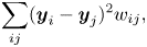
where $w_{ij}$ represents the similarity between the training data $\boldsymbol {x}_i$
 and $\boldsymbol {x}_j$
 . If $w_{ij}$
 is non-zero, $\boldsymbol {y}_i$
 and $\boldsymbol {y}_j$
 must be close to each other, in order to minimize (1). Taking the data points in the feature space as nodes of a graph, an edge between nodes $i$
 and $j$
 has a weight of $w_{ij}$
 , which is not zero, if they are close to each other. In the literature, we have found three different ways to determine the local geometry of a data point:
1 $\boldsymbol {\varepsilon }$
-neighborhood: this uses the distance to determine the closeness. Given $\varepsilon \in \mathbb {R}$, $\varepsilon$-neighborhood chooses the data points that fall within the circle around $\boldsymbol {x}_i$ with a radius $\varepsilon$. Those data points fall within the $\varepsilon$-neighborhood of $\boldsymbol {x}_i$ can be defined as
(2)\begin{equation} O(\boldsymbol{x}_i, \varepsilon) = \{\boldsymbol{x} | \ \|\boldsymbol{x} - \boldsymbol{x}_i\|^{2} < \varepsilon \}. \end{equation}
2 $\boldsymbol {k}$
-nearest neighborhood: another way of determining the local structure is to use the nearest neighborhood information. Presuming that the closest $k$ points of $\boldsymbol {x}_i$ would still be the closest data points of $\boldsymbol {y}_i$ in the projected manifold space, we can define a function $N(\boldsymbol {x}_i,k)$, which outputs the set of $k$-nearest neighbors of $\boldsymbol {x}_i$. Two types of neighborhood, with label information incorporated, are considered: $N(\boldsymbol {x}_i,k^{+} )$ and $N(\boldsymbol {x}_i,k^{-} )$, which represent the sets of $k$-nearest neighbors of $\boldsymbol {x}_i$ of the same label and of different labels, respectively.3 The class information: the class or label information is often used in supervised subspace methods. In a desired manifold subspace, the data points belonging to the class of $\boldsymbol {x}_i$
are to be projected such that they are close to each other, so as to increase the intra-class compactness. The data points belonging to other classes are projected, such that they will become farther apart and have larger inter-class separability. The class label information is often combined with either the $\varepsilon$-neighborhood or the $k$-nearest neighborhood.


The similarity graph is constructed by setting up edges between the nodes. There are different ways of determining the weights of the edges, considering the fact that the distance between two neighboring points can also provide useful information about the manifold. Given a sparse symmetric similarity matrix $\mathbf {W}$ , two variations have been proposed in the literature:
1 Binary weights: $w_{ij}=1$
if, and only if, the nodes $i$ and $j$ are connected by an edge, otherwise $w_{ij}=0$.2 Heat kernel ($t\in \mathbb {R}$
): if the nodes $i$ and $j$ are connected by an edge, the weight of the edge is defined as
(3)\begin{equation} w_{ij} = \text{exp}\Bigg (\frac{-\|\boldsymbol{x}_i-\boldsymbol{x}_j\|^{2}}{t} \Bigg ). \end{equation}


After constructing the similarity matrix with the weights, the minimization problem defined in (1) can be solved by using the spectral graph theory. Defining the Laplacian matrix $\mathbf {L} = \mathbf {D} - \mathbf {W}$ , where $\mathbf {D}$
 is the diagonal matrix whose entries are the column sum of $\mathbf {W}$
 , i.e. $d_{ii}=\sum _j w_{ij}$
 , the objective function is reduced to
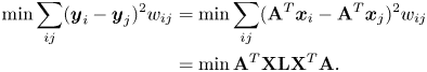
where $\mathbf {X}=[\boldsymbol {x}_1,\boldsymbol {x}_2,...,\boldsymbol {x}_m]$ , and $\mathbf {A}$
 is the projection matrix whose columns are the projection vectors. To avoid the trivial solution of the objective function, the constraint $\mathbf {A}^{T}\mathbf {X}\mathbf {D}\mathbf {X}^{T}\mathbf {A}=1$
 is often added. After specifying the objective function, the optimal projection matrix $\mathbf {A}$
 can be computed by solving the standard eigenvalue decomposition or generalized eigenvalue problem. Equation (4) can be solved by using Lagrange multiplier, as follows:
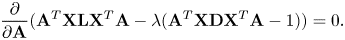
The solution is $(\mathbf {X}\mathbf {D}\mathbf {X}^{T})^{-1}\mathbf {X}\mathbf {L}\mathbf {X}^{T}\mathbf {A} = \lambda \mathbf {A}$ . The columns of $\mathbf {A}$
 should be the eigenvectors of the matrix $(\mathbf {X}\mathbf {D}\mathbf {X}^{T})^{-1} \mathbf {X}\mathbf {L}\mathbf {X}^{T}$
 , corresponding to the $d (d \ll D)$
 smallest non-zero eigenvalues.
1) Constructing the within-class and the between-class graph matrices
As mentioned in the previous section, one of the most popular graph-based subspace-learning methods is LPP [Reference Yan, Xu, Zhang, Zhang, Yang and Lin12], which uses an intrinsic graph to represent the locality information of the data points, i.e. the neighborhood information. The idea behind LPP is that if the data points $\boldsymbol {x}_i$ and $\boldsymbol {x}_j$
 are close to each other in the feature space, then they should also be close to each other in the manifold subspace. The similarity matrix $\mathbf {W}$
 for LPP can be defined as follows:
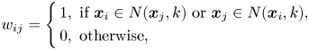
where $N(\boldsymbol {x}_j, k)$ represents the set of $k$
 -nearest neighbors of $\boldsymbol {x}_i$
 . One shortfall of the above formulation for $w_{ij}$
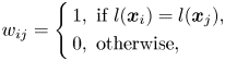
 is that it is an unsupervised method, i.e. not using any class-label information. Thinking that the label information can help to find a better separation between different class manifolds, supervised locality preserving projections (SLPP) was introduced in [Reference He and Niyogi13]. Denote $l(\boldsymbol {x}_i)$
 as the corresponding class label of the data point $\boldsymbol {x}_i$
 . SLPP uses either one of the following formulations:
Note that equation (7) does not include the neighborhood information to the adjacency graph, and the similarity matrices defined above can be constructed using the heat kernel. This strategy is also adopted in [Reference Cai, He, Zhou, Han and Bao19, Reference Jia, Liu, Hou and Kwong20] for graph construction. Orthogonal locality preserving projection (OLPP) [Reference Yu and Bhanu34] whose eigenvectors are orthogonal to each other is an extension of LPP. It is worth noting that, in our experiments we applied supervised orthogonal locality preserving projections (SOLPP), which is OLPP with its adjacency matrix including class information.
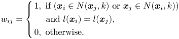
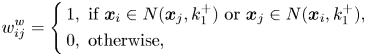
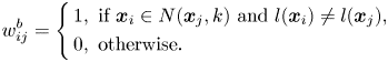
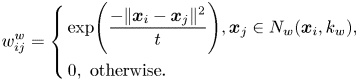
Yan et al. [Reference Belkin and Niyogi11] proposed a general framework for dimensionality reduction, named marginal Fisher analysis (MFA). MFA, which is based on graph embedding as LPP, uses two graphs, the intrinsic and penalty graphs, to characterize the intra-class compactness and the interclass separability, respectively. In MFA, the intrinsic graph $w_{ij}^{w}$ , i.e. the within-class graph, is constructed using the neighborhood and class information as follows:
where $k_1^{+}$ is the number of nearest neighbors of the same class of $\boldsymbol {x}_i$
 . Similarly, the penalty graph $w_{ij}^{b}$
 , i.e. the between-class graph, is constructed as follows:
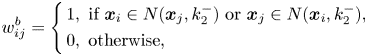
where $k_2^{-}$ is the number of nearest neighbors whose class is different from $\boldsymbol {x}_i$
 .
.
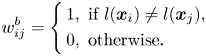
LSDA [Reference Li, Huang, Wang and Liu18] and improved locality-sensitive discriminant analysis (ILSDA) [Reference Cai and He35] are subspace-learning methods proposed in 2007 and 2015, respectively. They construct the similarity matrices in the same way, but LSDA uses binary weights, while ILSDA sets the weight of the edges using the heat kernel. The similarity matrices of LSDA are defined as follows:

It can be observed that the intrinsic and the penalty graphs of MFA, LSDA, and ILSDA are similar to each other. In MFA, the numbers of neighboring points for both the similarity matrices are known, i.e. $k_1$ and $k_2$
 . In LSDA and ILSDA, the $k$
 neighbors of $\boldsymbol {x}_i$
 are selected, which are then divided for constructing the within-class ($k^{+}$
 samples the same class as $\boldsymbol {x}_i$
 ) and the between-class matrices ($k^{-}$
 samples of other classes), i.e. $k=k^{+}+k^{-}$
 . Let $k_1$
 and $k_2$
 be the numbers of samples belonging to the same class and different classes, respectively, for MFA. It is worth noting that the equation $N(\boldsymbol {x}_i, k_1) \cap N(\boldsymbol {x}_i, k_2) = N(\boldsymbol {x}_1, k)$
 is not always true. This is because it is not necessarily true that $k^{+}=k_1$
 and $k^{-}=k_2$
 . Therefore, the neighboring points of $\boldsymbol {x}_i$
 in LSDA and ILSDA are not the same as MFA, even if $k=k_t= k_1+k_2$
 . However, the adjacency matrices constructed in the manifold learning methods are similar to each other. The main difference between the existing methods in the literature is in their definitions of the objective functions. We will elaborate on the differences in the objective functions in the next section.
LPMIP [Reference Chao, Ding and Liu16], proposed in 2008, uses the $\varepsilon$ -neighborhood condition, i.e. $O(\boldsymbol {x}_i,\varepsilon )$
 . Although it was originally applied as an unsupervised learning method, the class labels were used to construct the locality and non-locality information for facial expression recognition. In 2008, Li et al. [Reference Wang, Chen, Hu and Zheng17] proposed CMVM, which aims to keep the local structure of the data, while separating the manifold of the different classes farther apart. The local-structure graphs, i.e. the between-class graph and the dissimilarities graph, are defined as follows:

As (13) and (14) show, the within-class matrix of CMVM only preserves the local structure of the whole data, while the between-class matrix only uses the class label to increase the separability of different class manifolds. In 2015, an extension of CMVM, namely CMVM+ [Reference Yi, Zhang, Kong and Wang36], was proposed to overcome the obstacles of CMVM. CMVM+ adds the class information and neighborhood information to the similarity matrices. The updated version of the graphs can be written as follows:

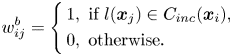
where $C_{inc}(\boldsymbol {x}_i)$ is a set of neighboring points belonging to different classes, i.e. $l(\boldsymbol {x}_i )\ne l(\boldsymbol {x}_j )$
 . More details of the function $C_{inc}(\boldsymbol {x}_i)$
 can be found in [Reference Yi, Zhang, Kong and Wang36].
In 2011, multi-manifolds discriminant analysis (MMDA) [Reference Zhao, Han, Zhang and Bai37] was proposed for image feature extraction, and applied to face recognition. The idea behind MMDA is to keep the points from the same class as close as possible in the manifold space, with the within-class matrix defined as follows:

MMDA also constructs a between-class matrix in order to separate the different classes from each other. The difference between the between-class matrix of MMDA and the other subspace methods is that its graph matrix is constructed by not taking all the data points as nodes, but rather calculating the weighted centers of different classes by averaging all the data points belonging to the classes under consideration. Let $\mathbf {M}=[\tilde {\boldsymbol {m}}_1,\tilde {\boldsymbol {m}}_2,\ldots,\tilde {\boldsymbol {m}}_c]$ be the class-weighted centers, where $c$
 is the number of classes. Then, the between-class matrix of MMDA can be written as:

In Table 2, a summary is given of the within-class graph and between-class graph for the subspace-learning methods, reviewed in this paper. In this table, the determination of the nearest neighbors; whether or not the class information being used, i.e. supervised or unsupervised learning; and the formulation of the weights are provided for the within-class graph and the between-class graph. For LPP/OLPP/SLPP/SOLPP, only the within-class graph is considered, so the neighborhood, class information, and weight for the between-class graph are listed as n/a (not available).
Table 2. Comparison of the within-class graph and the between-class graph for different subspace-learning methods
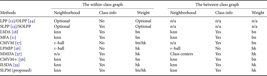
bn: binary weights, hk: heat kernel, knn: $k$ -nearest neighbor.
2) Defining the objective functions
Table 3 summarizes the objective functions of the approaches reviewed in the previous section, as well as the constraints used. We can see that SLPP has only one Laplacian matrix defined in its objective function, because it constructs one similarity matrix only, while all the other methods have two matrices: one is based on the intrinsic graph, and the other on the penalty graph.
Table 3. Comparison of the objective functions used by different subspace methods
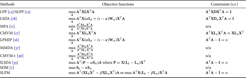
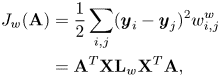
In general, there are two ways of defining the objective functions with the intrinsic and the penalty matrices. The first one utilizes the Fisher criterion to maximize the ratio between the scattering of the between-class and that of the within-class Laplacian matrices. MFA, MMDA, and CMVM+ employ the Fisher criterion. Although the application of the Fisher criterion shows its robustness, it involves taking the inverse of a high-dimensional matrix to solve a generalized eigenvalue problem. To solve this problem, LSDA, LPMIP, and our proposed SLMP define their objective functions as the difference between the intrinsic and the penalty-graph matrices, while MMC and SDM use the difference between the inter-class and the intra-class scatter matrices.
As shown in Table 3, ILSDA adopts a similar objective function to LSDA, but with a difference that the within-class scatter matrix is included in the objective function. The within-class scatter matrix $\mathbf {S}_w$ – as used in LDA – indicates the compactness of the data point in each class. ILSDA uses the scatter matrix to project outliers closer to the class centers under consideration. The objective function of ILSDA is defined as follows:

where $\mathbf {P} = \mathbf {X}(\mathbf {L}_b - \mathbf {L}_w)\mathbf {X}^{T}$ , as defined in the objective function of LSDA. CMVM, unlike other methods which aim to minimize the within-class spread, intends to maintain the within-class structure for each class by defining a constraint, i.e. $\mathbf {A}^{T}\mathbf {X}\mathbf {L}_{w}\mathbf {X}^{T}\mathbf {A} = \mathbf {X}^{T}\mathbf {L}_{w}\mathbf {X}$
 , while increasing the inter-class separability with the following objective function:

where $\mathbf {L}_{w}$ and $\mathbf {L}_{b}$
 are the within-class and the between-class Laplacian matrices, respectively.
B) Deep subspace learning
Deep subspace learning generally employs multi-level subspace mapping to extract abstract features from an image. One of the most commonly used deep subspace learning frameworks is PCANet [Reference Yang, Sun and Zhang38], proposed by Chan et al., which iteratively utilizes the convolutional layers with the PCA filters to learn image representations. They further proposed LDANet [Reference Yang, Sun and Zhang38] to enhance the feature representations, based on the Fisher criterion. To tackle the efficiency problem caused by cascading the PCA or LDA filters, binary hashing, and block-wise histograms, the pooling operation is introduced into the deep frameworks to reduce the dimensionality of the extracted features, such as the general pooling [Reference Chan, Jia, Gao, Lu, Zeng and Ma39], the rank-based average pooling [Reference Hu, Yang, Yi, Kittler, Christmas, Li and Hospedales40], and the spatial pyramid pooling [Reference Shi, Ye and Wu41].
The above-mentioned methods aim to learn linear mappings to form the subspace for describing facial images. However, these methods lack the capacity to describe the complexity of facial expressions in real-world scenarios. Deep convolutional neural networks (DCNNs) provide an alternative to learning the subspace by using more complicated nonlinear mappings. Recently, DCNNs have shown their superiority in various computer vision tasks, including image classification [Reference He, Zhang, Ren and Sun42, Reference Krizhevsky, Sutskever and Hinton43], object detection [Reference He, Zhang, Ren and Sun44, Reference Ren, He, Girshick and Sun45], and image restoration [Reference Redmon, Divvala, Girshick and Farhadi46, Reference Zhang, Zuo, Chen, Meng and Zhang47]. A DCNN model is generally trained by minimizing an empirical risk as follows:

where $f_{\theta }$ is the nonlinear mapping function with its trainable parameters $\theta$
 under an objective function $\mathcal {L}$
 , and $\boldsymbol {x}_{i}$
 represents an input signal, with its corresponding label $l(\boldsymbol {x}_{i})$
 . In terms of the facial expression recognition task, the objective function is generally defined as the softmax loss $\mathcal {L}_{\text {sfm}}$
 as follows:

where $\boldsymbol {y}_i = f_{\theta }(\boldsymbol {x}_i)$ is the learned deep feature for sample $\boldsymbol {x}_i$
 , and $\boldsymbol {W}$
 and $\boldsymbol {b}$
 are the trainable kernels and bias of the output layer, respectively. However, the features learned under the softmax loss can achieve class separability only, but there is no guarantee for discriminability. Therefore, deep subspace regularizers are proposed to introduce the within-class and the between-class variances as the additional penalty into the objective function. By this means, the learned deep features become more discriminative and generalized for recognizing new unseen query faces. Similar to the traditional subspace learning algorithms introduced in Section A), deep subspace learning aims to learn a subspace that characterizes face features by widening the between-class differences and compacting the within-class variations. In this paper, we mainly focus on the regularization-based deep subspace learning methods.
1) Regularization for deep subspace learning
Wen et al. [Reference Li and Deng28] proposed the Center loss for face recognition, which aims to minimize the within-class variations while keeping the features of different classes separable. To this end, the Center loss minimizes the distance between each sample and its corresponding class center in the latent space, as follows:
where $\boldsymbol {c}_{l(\boldsymbol {x}_i)}$ denotes the center or mean deep feature for the class $l(\boldsymbol {x}_i)$
 , and $m$
 is the batch size. This Center loss can effectively describe the within-class variations. However, the between-class variations are not sufficiently considered, which may result in the overlaps between the clusters of different classes in the latent space. Therefore, in order to enlarge the between-class distance, Cai et al. [Reference Zhao, Liu, Xiao, Lun and Lam26] proposed the Island loss, which further introduces a regularization term to penalize the pairwise distance between the centers of different classes, as follows:
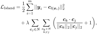
where $\lambda$ is a hyperparameter controlling the trade-off between the intra-class and the inter-class variations, and $N$
 denotes the set of class centers in the learned subspace. The second term in this loss function is normalized to the range $[0, 2]$
 . Compared to the Center loss, the Island loss further maximizes the distance between the centers of the different classes. This effectively addresses the overlap issue and significantly improves the feature discriminative ability.
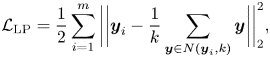
On the contrary, local information is essential for the formation of a feature space with better generalization [Reference Cai, Meng, Khan, Li, O'Reilly and Tong27]. Inspired by SLPP [Reference He and Niyogi13], Li et al. [Reference Cai, Meng, Khan, Li, O'Reilly and Tong27] proposed the locality preserving (LP) loss, and established the deep locality preserving-CNN (DLP-CNN), which aims to guarantee the local consistency in the learned subspace. The locality preserving loss is formulated as follows:

where the similarity matrix $S_{i,j}$ is defined, based on SLPP [Reference He and Niyogi13], as follows:
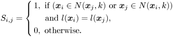
However, to calculate the sum of the pairwise distances, the entire training set is required to be fed to the network for training in each iteration, which is computationally intensive. Therefore, Li et al. [Reference Cai, Meng, Khan, Li, O'Reilly and Tong27] further proposed to make an approximation by only searching the $k$ nearest neighbors of $\boldsymbol {y}_i$
 in each iteration. Thus, the locality preserving loss is reformulated as follows:
where $N(\boldsymbol {y}_i, k)$ denotes the ensemble of the $k$
 -nearest neighbors of the feature point $\boldsymbol {y}_i$
 with the same label. Equation (27) effectively characterizes the “local” within-class scatters, because the samples from the same class are forced to be close to each other in the latent subspace. Moreover, if we set the number of neighbors $k = N_j$
 , where $N_j$
 is the number of samples from the $j$
 -th class in the entire training set, the locality preserving loss becomes the Center loss. Thus, the Center loss can be regarded as a special case of the locality preserving loss.
However, the locality preserving loss, similar to the Center loss, has not sufficiently considered the local inter-class variations, and only adopts the softmax loss to make the features separable. Therefore, in this paper, we reformulate the proposed SLPM as an additional regularization, i.e. soft locality preserving (SLP) loss, for training the CNN models, in order to learn more discriminative representations for facial expressions. We summarize the above-mentioned deep subspace-learning methods in Table 4.
Table 4. Comparison of the different deep subspace-learning regularizers
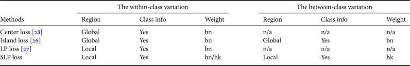
bn: binary weights, hk: heat kernel.
2) Learning scheme
Both the center-based [Reference Zhao, Liu, Xiao, Lun and Lam26, Reference Li and Deng28] and the locality-based [Reference Cai, Meng, Khan, Li, O'Reilly and Tong27] methods need to take all the training samples, which are fed to the network, to calculate the respective class centers in training. This is not only time-consuming, but also impractical in real-world applications. To address this problem, a mini-batch-based training scheme is necessary to reliably update or compute the centers for those additional regularization terms.
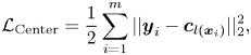
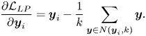
For the center-based approaches, Wen et al. [Reference Zhao, Liu, Xiao, Lun and Lam26] proposed to compute the gradients of the class centers based on the samples in a mini-batch only. Specifically, the class centers are first randomly initialized at the beginning of the training process. In each iteration, the gradient of $\mathcal {L}_{\text {Center}}$ with respect to the FV $\boldsymbol {y}_i$
 is calculated as follows:

and then the centers are updated in each iteration as follows:

where $\delta (\text {condition}) = 1$ if the condition is satisfied, and $\delta (\text {condition}) = 0$
 , otherwise. By this means, the randomly initialized class centers can be optimized during the mini-batch training. Similarly, the center gradients in the Island loss can be computed as follows:
where $|N|$ denotes the total number of expression classes.
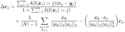
As the center-based method is just a special case of the locality-based method, the center updating scheme in DLP-CNN [Reference Cai, Meng, Khan, Li, O'Reilly and Tong27] can be defined similarly, as follows:
It is worth noting that all the above-mentioned regularizers are cooperating with the softmax loss defined in equation (22) to jointly supervise the subspace learning process.
III. SOFT LOCALITY PRESERVING MAP
In this section, we introduce the proposed method, SLPM, with its formulation and connection to the previous studies. Then, we will also describe the local descriptors used for facial expression recognition in our experiments. Finally, we extend SLPM to deep learning, and describe the deep network architecture for learning discriminative features supervised by the soft locality preserving loss.
A) Formulation of the SLPM
Similar to other manifold-learning algorithms, two graph-matrices, i.e. the between-class matrix $\mathbf {W}_b$ and the within-class matrix $\mathbf {W}_w$
 , are constructed to characterize the discriminative information, based on the locality and class-label information. Given $m$
 data points $\{\boldsymbol {x}_1, \boldsymbol {x}_2, \dots , \boldsymbol {x}_m \} \in \mathbb {R}^{D}$
 and their corresponding class labels $\{l(\boldsymbol {x}_1 ), l(\boldsymbol {x}_2 ), \dots , l(\boldsymbol {x}_m )\}$
 , we denote $N_w (\boldsymbol {x}_i, k_w ) = \{\boldsymbol {x}_i^{w_1}, \boldsymbol {x}_i^{w_2}, \dots ,x_i^{w_{k_w}} \}$
 as the set of $k_w$
 -nearest neighbors with the same class label as $\boldsymbol {x}_i$
 , i.e. $l(\boldsymbol {x}_i) = l(\boldsymbol {x}_i^{w_1}) = l(\boldsymbol {x}_i^{w_2} ) = \dots = l(\boldsymbol {x}_i^{w_{k_w}} )$
 , and $N_b(\boldsymbol {x}_i,k_b )$ $= \{\boldsymbol {x}_i^{b_1}, \boldsymbol {x}_i^{b_2}, \dots ,\boldsymbol {x}_i^{b_{k_b}}\}$
 as the set of its $k_b$
 nearest neighbors with different class labels from $\boldsymbol {x}_i$
 , i.e. $l(\boldsymbol {x}_i) \neq l(\boldsymbol {x}_i^{w_j} )$
 , where $j=1,2,\dots ,k_b$
 . Then, the inter-class weight matrix $\mathbf {W}_b$
 and the intra-class weight matrix $\mathbf {W}_w$
 can be defined as below:

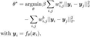
SLPM is a supervised manifold-learning algorithm, which aims to maximize the between-class separability, while controlling the within-class spread with a control parameter $\beta$ used in the objective function. Consider the problem of creating a subspace, such that data points from different classes, i.e. represented as edges in $\mathbf {W}_b$
 , stay as distant as possible, while data points from the same class, i.e. represented as edges in $\mathbf {W}_w$
 , stay close to each other. To achieve this, two objective functions are defined as follows:


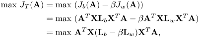
Equation (34) ensures that the samples from different classes will stay as far as possible from each other, while equation (35) is to make samples from the same class stay close to each other after the projection. However, as shown in [Reference Zhao, Lam and Lun48] and [Reference Li, Jiang and Zhang7], small variations in the manifold subspace can lead to overfitting in training. To overcome this problem, we add the parameter $\beta$ to control the intra-class spread. Note that, the method SDM in [Reference Li, Jiang and Zhang7] uses the within-class scatter matrix $\mathbf {S}_w$
 – as defined for LDA – to control the intra-class spread. In our proposed method, we adopt the graph-embedding method, which uses the locality information about each class, in addition to the class information. Hence, the two objective functions equations (34) and (35) can be combined as follows:

where $\mathbf {A}$ is a projection matrix, i.e. $\mathbf {Y} = \mathbf {A}^{T}\mathbf {X}$
 and $\mathbf {X} = [\boldsymbol {x}_1, \boldsymbol {x}_2, \dots , \boldsymbol {x}_m]$
 . Then, the between-class objective function $J_{b}(\mathbf {A})$
 can be reduced to

where $\mathbf {L}_b = \mathbf {D}_b - \mathbf {W}_b$ is the Laplacian matrix of $\mathbf {W}_b$
 and $d_{b_{ii}} = \sum _j w_{ij}^{b}$
 is a diagonal matrix. Similarly, the within-class objective function $J_{w}(\mathbf {A})$
 can be written as
where $\mathbf {L}_w = \mathbf {D}_w - \mathbf {W}_w$ and $d_{w_{ii}} = \sum _j w_{ij}^{w}$
 . If $J_{b}$
 and $J_{w}$
 are substituted into equation (36), the objective function becomes as follows:
which is subject to $\mathbf {A}^{T} \mathbf {A}-\mathbf {I} = 0$ , so as to guarantee orthogonality. By using Lagrange multiplier, we obtain

By computing the partial derivative of $\text {L}(\mathbf {A})$ , the optimal projection matrix $\mathbf {A}$
 can be obtained, as follows:
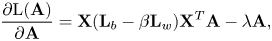
i.e. $\mathbf {X}(\mathbf {L}_{b} - \beta \mathbf {L}_{w}) \mathbf {X}^{T}\mathbf {A} = \lambda \mathbf {A}$ . The projection matrix $\mathbf {A}$
 can be obtained by computing the eigenvectors of $\mathbf {X}(\mathbf {L}_{b} - \beta \mathbf {L}_{w}) \mathbf {X}^{T}$
 . The columns of $\mathbf {A}$
 are the $d$
 leading eigenvectors, where $d$
 is the dimension of the subspace. The proposed SLPM algorithm requires computing the pairwise distance between the samples for construction of the within-class and between-class matrices. The complexity of this is $\mathcal {O}(m^{2})$
 , where $m$
 is the number of training samples. In addition, the complexity of calculating the eigenvalue decomposition is $\mathcal {O}(m^{3})$
 . LDA, LPP, MFA, and other manifold-learning algorithms, whose objective functions have a similar structure, lead to a generalized eigenvalue problem. Such methods suffer from the matrix-singularity problem, because the solution involves computing the inverse of a singular matrix. Although computing the inverse of a matrix also involves a time complexity of $\mathcal {O}(m^{3})$
 , the proposed objective function is designed in such a way as to overcome this singularity problem. However, in our algorithm, PCA is still applied to data, so as to reduce its dimensionality and to reduce noise.
B) Intra-class spread
As we have mentioned before, the manifold spread of the different classes can affect the generalizability of the learned classifier. To control the spread of the classes, the parameter $\beta$ is adjusted in our proposed method, like SDM. Figure 1 shows the change in the spread of the classes when $\beta$
 increases. We can see that increasing $\beta$
 will also increase the separability of the data, e.g. the training data is located at almost the same position in the subspace when $\beta = 1000$
 .
.
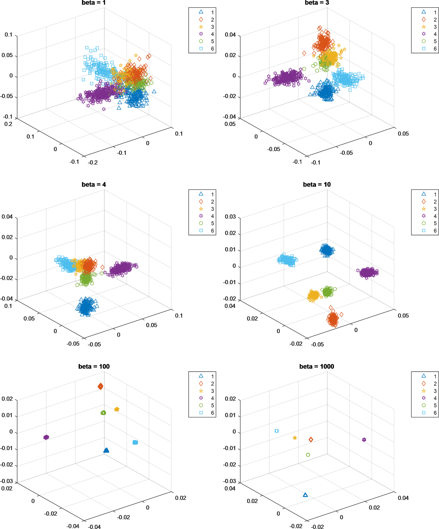
Fig. 1. Spread of the respective expression manifolds when the value of $\beta$ increases from 1 to 1000: (1) anger, (2) disgust, (3) fear, (4) happiness, (5) sadness, and (6) surprise.
C) Relations to other subspace-learning methods
As discussed in Section 2, there have been extensive studies on manifold-learning methods. They share the same core idea, i.e. using locality and/or label information to define an objective function, so that the data can be represented in a specific way after projection.
There are two main differences between SLPM and LSDA. First, LSDA defines their objective function as a subtraction of two objective functions like SLPM. However, LSDA imposes the constraint $\mathbf {A}^{T} \mathbf {XD}_w \mathbf {X}^{T} \mathbf {A} = \mathbf {I}$ , which results in a generalized eigenvalue problem. As we mentioned in Section 2, the generalized eigenvalue problem suffers from the computational cost of calculating an inverse matrix. SLPM only determines the orthogonal projections, with the constraint $\mathbf {A}^{T} \mathbf {A} - \mathbf {I}=0$
 . Therefore, SLPM can still be computed by eigenvalue decomposition, without requiring computing any inverse matrix. Second, LSDA finds the neighboring points followed by determining whether the considered neighboring points are of the same class or of different classes. This may lead to an unbalanced and unwanted division of neighboring points, simply because of the fact that a sample point may be surrounded by more samples belonging to the same class than samples with different class labels. In order not to lose locality information in such a case, SLPM defines two parameters $k_1$
 and $k_2$
 , which are the numbers of neighboring points belonging to the same class and different classes, respectively. In other words, the numbers of neighboring points belonging to the same class and different classes can be controlled.
Both SDM and ILSDA also consider the intra-class spread when defining the objective function. SDM controls the level of spread by applying a parameter to the within-class scatter matrix $\mathbf {S}_w$ . However, it only uses the label information about the training data – its scatter matrices do not consider the local structure of the data. Our proposed SLPM aims to include the locality information by employing graph embedding in our objective functions. Therefore, SLPM is a graph-based version of SDM. ILSDA uses both the label and neighborhood information represented in the adjacent matrices, and also aims to control the spread of the classes. However, ILSDA achieves this by adding the scatter matrix $\mathbf {S}_w$
 to its objective function. In our algorithm, we propose controlling the spread with the within-class Laplacian matrix $\mathbf {L}_w$
 , without adding a separate element to the objective function.
D) Deep soft locality preserving learning
The objective function of SLPM, as described in equation (36), is extended for deep learning for learning more discriminant deep features. The objective function is formulated as a loss function, which aims to minimize the within-class variation, while maximizing the between-class difference. In equation (36), $\boldsymbol {y}$ is the feature in the learned subspace formed by a linear projection matrix $\mathbf {A}$
 . $w^{b}$
 and $w^{w}$
 represent the similarity between the between-class samples and the within-class samples, respectively, in a local neighborhood. If we employ a deep neural network to extract the FV from each sample, denoted as $\boldsymbol {y}_i = f_{\theta }(\boldsymbol {x}_i)$
 , the learning objective becomes as follows:
where the similarity of the inter-class and intra-class samples, i.e. $w^{b}_{i,j}$ and $w^{w}_{i,j}$
 , are computed based on equations (32) and (33), respectively.
Similar to DLP-CNN [Reference Cai, Meng, Khan, Li, O'Reilly and Tong27], the learned feature $\boldsymbol {y}_i$ should be updated iteratively during the mini-batch training. Therefore, we adopt the same approximation in [Reference Cai, Meng, Khan, Li, O'Reilly and Tong27] to only consider the $k$
 nearest neighbors of each feature $\boldsymbol {y}_i$
 , and reformulate the objective function as follows:
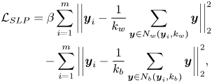
where $\beta$ also controls the intra-class spread, which affects the generalization of the resultant feature extractor. Equation (43) represents the proposed soft locality-preserving (SLP) loss, which effectively characterizes the within-class and the between-class variations in a local region, and consequently enhances the discriminability and the generalization of the model.
We follow the learning strategy in [Reference Cai, Meng, Khan, Li, O'Reilly and Tong26–Reference Wen, Zhang, Li and Qiao28], and adopt the joint supervision of the softmax and the SLP loss to train up the CNN model, named SLP-CNN, for subspace learning. Thus, the overall loss function is defined as follows:

where $\lambda$ balances the trade-off between the two loss terms. The softmax loss guarantees the separability of the global scatter, while the SLP loss enhances the discriminative power based on local scatters.
To learn the deep discriminative features with respect to facial expressions, we establish a convolutional neural network with the same architecture as DLP-CNN [Reference Cai, Meng, Khan, Li, O'Reilly and Tong27], whose structure is shown in Table 5. We adopt an 18-layer CNN with the ReLU [Reference Kung, Tu and Hsu49] activation function. The last fully connected layer in Table 5 is the softmax layer for introducing the softmax supervision. It can be seen from the table that we extract a 2000-dimensional FV from each facial sample. The SLP loss is computed based on these 2000-dimensional FVs, produced by the second last layer. We summarize our proposed learning algorithm, SLP-CNN, as shown in Algorithm 1. In terms of the time complexity, the proposed algorithm only affects that in the training stage, and thus, brings no burden to the inference stage. The proposed SLP loss requires computing the pairwise distance between the samples doing training. Therefore, the time complexity in a mini-batch is described as $\mathcal {O}(m^{2})$ . As a comparison, the LP loss requires computing the distance between samples in the same cluster, whose computation should be $\mathcal {O}(m'^{2})$
 , where $m'$
 denotes the number of samples belonging to the same class in a mini-batch.
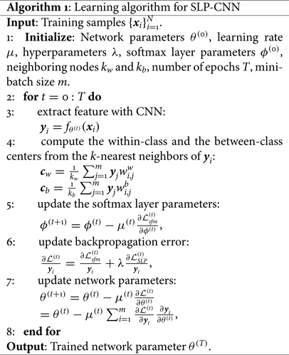
Table 5. Network architecture for learning discriminative features supervised by the soft locality preserving loss
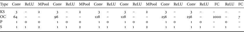
KS, OC, P, and S refer to the kernel size, output channel, padding, and stride, respectively.
IV. FEATURE DESCRIPTORS AND GENERATION
In this section, we will first present the descriptors used for representing facial images for expression recognition, then investigate the use of face images with low-intensity and high-intensity expressions for manifold learning, which represent the corresponding samples at the core and boundary of the manifold for an expression. After that, we will introduce our proposed feature-generation algorithm.
A) Descriptors
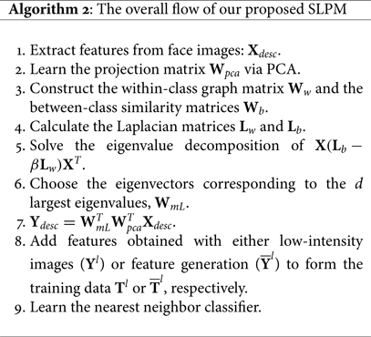
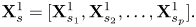
Recent research has shown that local features can achieve higher and more robust recognition performance than by using global features, such as eigenfaces and Fisherfaces, and intensity values. Therefore, in order to show the robustness of our proposed method, four different commonly used local descriptors for facial expression recognition, local binary pattern (LBP) [Reference Maas, Hannun and Ng50, Reference Ojala, Pietikäinen and Harwood51], local phase quantization (LPQ) [Reference Shan, Gong and McOwan52], pyramid of histogram of oriented gradients [Reference Ojansivu and Heikkilä53], and Weber local descriptor (WLD) [Reference Bosch, Zisserman and Munoz54], are considered in our experiments. These descriptors can represent face images, in terms of different aspects such as intensity, phase, shape, etc., so that they are complementary to each other [Reference Chen55]. As shown in Algorithm 2, features are extracted using one of the above-mentioned local descriptors, followed by the subspace learning with SLPM and a feature-generation method.
B) Feature generation
Features in a projected subspace still have a high dimension. A large number of samples for each expression is necessary in order to accurately represent its corresponding manifold. This is similar to deep learning in that an extremely large amount of training samples are necessary to solve the overfitting problem. For deep learning, data augmentation is carried out to generate more samples from a single training image. However, for conventional subspace analysis methods, data augmentation does not work properly. To achieve effective learning, it is necessary to generate more features located near the manifold boundaries. Then, more accurate decision boundaries can be determined for accurate facial expression. In other words, feature augmentation should be performed, rather than data augmentation.
Video sequences with face images, changing from neutral expression to a particular expression, are used for learning. Let $f_{i,\theta }$ denote the frame index of the face image of expression intensity $\theta$
 ($0\leq \theta \leq 1$
 , $0 = \text {neutral expression}$
 and $1 = \text {the highest intensity of an expression}$
 , i.e. the peak expression) of the sequence $S_i$
 in a dataset of $m$
 video sequences. Let $x_i^{\theta } \in \mathbb {R}^{D}$
 be the FV extracted from the $f_{i,\theta }$
 -th frame of the sequence $S_i$
 . The frame index $f_{i,\theta }$
 can be calculated as follows:

where $n_i$ is the number of frames in the sequence $S_i$
 . Therefore, $\{\boldsymbol {x}_{1}^{1}, \boldsymbol {x}_{2}^{1},\dots , \boldsymbol {x}_{m}^{1} \} \in \mathbb {R}^{D}$
 are the FVs extracted from the face images with high-intensity expressions, i.e. the last frames of the $m$
 video sequences. Suppose that $\{ \boldsymbol {x}_{1}^{\xi }, \boldsymbol {x}_{2}^{\xi },\dots , \boldsymbol {x}_{m}^{\xi } \}$
 are the FVs extracted from the corresponding low-intensity images, and the corresponding frame number in the respective video sequences is $f_{i,\xi }$
 . In our algorithm, we use a different set of $\xi$
 values, where $0.6 \leq \xi \leq 0.9$
 , to learn the different expression manifolds.
1) Manifold learning with high- and low-intensity training samples
A projection matrix $\mathbf {A}$ that maps the FVs $\mathbf {X}^{1} = [\boldsymbol {x}_1^{1}, \boldsymbol {x}_2^{1},\dots , \boldsymbol {x}_m^{1} ]$
 to a new subspace is first calculated using SLPM. The corresponding projected samples are denoted as $\mathbf {Y}^{1} = [\boldsymbol {y}_1^{1}, \boldsymbol {y}_2^{1},\dots , \boldsymbol {y}_m^{1} ]$
 , i.e. $\boldsymbol {y}_i^{1} = \mathbf {A}^{T} \boldsymbol {x}_i^{1}$
 . Then, the same projection matrix $\mathbf {A}$
 is used to map the low-intensity FVs $\mathbf {X}^{\xi }=[\boldsymbol {x}_1^{\xi },\boldsymbol {x}_2^{\xi },\dots ,\boldsymbol {x}_m^{\xi } ]$
 , i.e. $\boldsymbol {y}_i^{\xi } = \mathbf {A}^{T} \boldsymbol {x}_i^{\xi }$
 , which should lie on the boundary of the corresponding expression manifold. The high-intensity and low-intensity samples in the subspace form a training matrix, denoted as $\mathbf {T}_{\xi }$
 , as follows:

where $\xi (0\leq \xi \leq 1)$ represents the intensity of the low-intensity images. Figures 2(b) and (c) demonstrate the training data $\mathbf {T}_{\xi }$
 with two different values of $\xi$
 on the CK+ database.
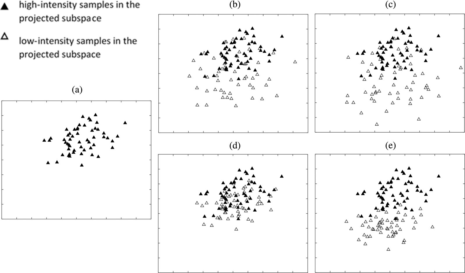
Fig. 2. Representation of the FVs of happiness (HA) on the CK+ database, after SLPM: (a) HA, i.e. high-intensity expression samples are applied to SLPM, (b) HA+ low intensity FV with $\xi =0.9$ , (c) HA+ low intensity FV with $\xi =0.7$
 , (d) HA+ generated FV with $\theta _{ne}=0.9$
 , and (e) HA+ generated FV with $\theta _{ne}=0.7$
 .
.
Conventional manifold-learning methods map training samples, irrespective of how strong the expressing images are, as close as possible after transformation. This results in limited performance in terms of generalization. In our feature-generation algorithm, the subspace learning method, SLPM, is first applied to features extracted from high-intensity expressions. Then, features extracted from low-intensity expressions are mapped to the learned subspace. As observed in Fig. 3, features extracted from low-intensity expressions are located farther from the core samples (formed by high-intensity expressions) and near the boundary of the manifolds after the mapping.
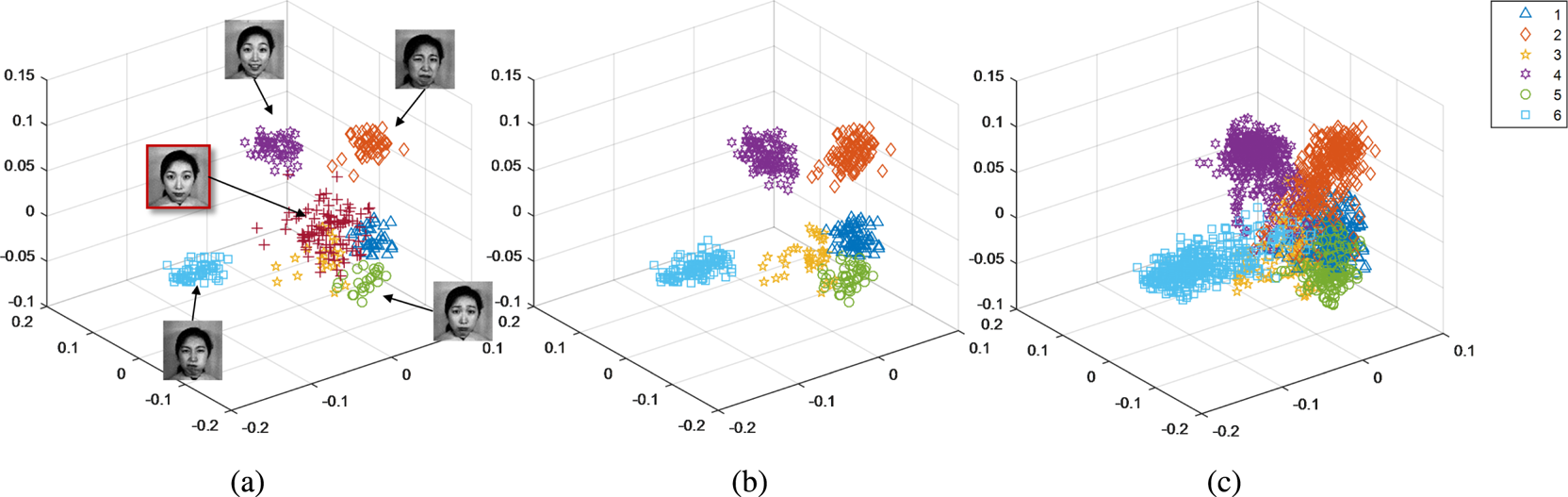
Fig. 3. Subspace learned using SLPM, with local descriptors “LP,” based on the dataset named CK+: (a) the mapped features extracted from high-intensity expression images and neutral face images, (b) the mapped features extracted from high-intensity and low-intensity ($\xi =0.7$ ) images, and (c) the mapped features extracted from high-intensity and low-intensity ($\xi =\{0.9, 0.8, 0.7, 0.6, 0.5, 0.4\}$
 ) images.
Let $\{\boldsymbol {x}_{s_1}^{0}, \boldsymbol {x}_{s_2}^{0},\dots ,\boldsymbol {x}_{s_p}^{0} \} \in \mathbb {R}^{D}$ be the set of FVs extracted from neutral face images, where $\boldsymbol {x}_{s_i}^{0}$
 is the FV of the neutral face image belonging to the subject $s_i$
 , and $p$
 is the number of the subjects in the dataset. The expression images of the subject $s_i$
 are denoted as

where $r$ is the number of expression images belonging to $s_i$
 and $x_{s_{i,j}}^{1}$
 is the FV extracted from the $j$
 -th expression image of $s_i$
 . Then, the feature matrix for all the expressions is formed as follows:
The proposed sample-generation method operates in the learned subspace. Thus, the FVs extracted from the neutral face images and the expression images are all mapped to the learned subspace using the projection matrix $\mathbf {A}$ learned from $\mathbf {X}^{1}_{s}$
 , as follows:


Equations (49) and (50) represent the set of FVs of high-intensity expressions and neutral expressions of all subjects, respectively, in the subspace.
The proposed feature-generation method generates low-intensity FVs based on vector-pairs selected from two different sets: (1) vector-pairs from $\mathbf {Y}_{s_i}^{1}$ and (2) vector-pairs from $\mathbf {Y}_{s_i}^{1}$
 and $\boldsymbol {y}_{s_i}^{0}$
 . In the following sections, we will describe the feature-generation method with respect to two different vector-pairs.
2) Vector-pairs from $\mathbf {Y}_{s_i}^{1}$ and $\mathbf{y}_{s_i}^{0}$


Let $\overline {\mathbf {Y}}_{s_i}^{\theta _{ne}} = [\boldsymbol {y}_{s_{i,1\to 0}}^{\theta _{ne}}, \boldsymbol {y}_{s_{i,2\to 0}}^{\theta _{ne}}, \dots , \boldsymbol {y}_{s_{i,r\to 0}}^{\theta _{ne}}]$ be the feature matrix of possible low-intensity expressions with an intensity of $\theta _{ne} (0 < \theta _{ne} < 1)$
 belonging to the subject $s_i$
 , where $\boldsymbol {y}_{s_{i,j\to 0}}^{\theta _{ne}}$
 is the corresponding low-intensity FV generated using $\boldsymbol {y}_{s_{i,j\to 0}}^{1}$
 and $\boldsymbol {y}_{s_{i}}^{0}$
 . In the rest of the paper, the arrow “$\to$
 ” indicates the direction of the FVs to be generated, with $0$
 and $1$
 being a neutral face image and a face image with the highest intensity, respectively. $\boldsymbol {y}_{s_{i,j\to 0}}^{\theta _{ne}}$
 means that the FV is generated in the direction from $\boldsymbol {y}_{s_{i,j}}^{1}$
 to $\boldsymbol {y}_{s_{i}}^{0}$
 where $\boldsymbol {y}_{s_{i,j}}^{1}$
 is the mapped FV extracted from the $j$
 -th expression image of $s_i$
 .
.
A set of FVs extracted from an expression video sequence, which starts from a neutral-expression face to the highest intensity of an expression, can be perceived as a path from the reference center, i.e. the neutral manifold, to a particular expression manifold wherein the distance of an expression manifold from the center is directly proportional to the intensity of the expression [Reference Turan and Lam56]. Therefore, for databases consisting of only static expression images, the feature matrix of possible low-intensity expressions can be obtained by assuming that the relation between the distance from $\boldsymbol {y}_{s_{i,j\to 0}}^{\theta _{ne}}$ to $\boldsymbol {y}_{s_i}^{0}$
 and the expression intensity is linear. As illustrated in Fig. 4(a), the low-intensity FV $\boldsymbol {y}_{s_{i,j\to 0}}^{\theta _{ne}}$
 , belonging to $s_i$
 , can be computed as follows:


Fig. 4. Representation of the sample-generation process based on (a) FVs extracted from high-intensity images and neutral-face images, and (b) FVs extracted from high-intensity images.
Figures 2(d) and (e) outline the training data with the feature generation using neutral images when $\theta _{ne}=0.9$ and $\theta _{ne}=0.7$
 , respectively. As seen in Fig. 2, both the absolute low-intensity FVs and the possible low-intensity FVs generated by linear interpolation have a similar structure.
3) Vector-pairs from $\mathbf {Y}_{s_i}^{1}$

The respective expression manifolds can be far from each other in the learned subspace. For this reason, more features between expression manifolds are also needed. In the previous section, we proposed the idea that the FVs extracted from low-intensity expression images should be distant from the corresponding manifold center, thus, this can enhance the generalizability of the learned manifold. Using a similar idea, more features that are distant from the manifold centers can be generated using vector-pairs from the feature matrix of high-intensity expressions of the same subject, $\mathbf {Y}_{s_i}^{1}$ , as illustrated in Fig. 4(b). A FV $\boldsymbol {y}_{s_{i,j\to k}}^{\theta _{exp}}$
 , which lies on the line from the $j$
 -th expression-vector of $s_i$
 , $\boldsymbol {y}_{s_{i,j}}^{1}$
 , to the $k$
 -th expression-vector of $s_i$
 , $\boldsymbol {y}_{s_{i,k}}^{1}$
 , with a weight $\theta _{exp} ( 0 < \theta _{exp} <1)$
 can be computed as follows:

Suppose that $c_{j}=l(\boldsymbol {y}_{s_{i,j}}^{1})$ and $c_k=l(\boldsymbol {y}_{s_{i,k}}^{1})$
 are the expression classes of the $j$
 -th and the $k$
 -th expression vectors, respectively, and $n_{i,c_j}$
 and $n_{i,c_k}$
 are the number of expression-vectors of expression classes $c_j$
 and $c_k$
 , respectively, belonging to subject $s_i$
 . Then, a total of $n_{i,c_j} \text { } n_{i,c_k}$
 FVs can be generated. The feature matrix consisting of the generated features using the pairs from $\mathbf {Y}_{s_i}^{1}$
 can be denoted as follows:

The training matrix, $\mathbf {T}_\theta$ , is updated to $\overline {\mathbf {T}}_\theta$
 , which is used as a static database, as follows:

where $\overline {\mathbf {Y}}_{ne}^{\theta _{ne}} = [\overline {\mathbf {Y}}_{s_{1,ne}}^{\theta _{ne}}, \overline {\mathbf {Y}}_{s_{2,ne}}^{\theta _{ne}}, \dots , \overline {\mathbf {Y}}_{s_{p,ne}}^{\theta _{ne}}]$ and $\overline {\mathbf {Y}}_{exp}^{\theta _{exp}} = [\overline {\mathbf {Y}}_{s_{1,exp}}^{\theta _{exp}}, \overline {\mathbf {Y}}_{s_{2,exp}}^{\theta _{exp}}, \dots , \overline {\mathbf {Y}}_{s_{p,exp}}^{\theta _{exp}}]$
 . In our experiments, we vary the $\theta _{ne}$
 and the $\theta _{exp}$
 values from 0.7 to 0.9. Algorithm 1 lists the overall flow of the proposed algorithm.
When an FV is generated, it is checked whether or not it is closest to its corresponding manifold class. Furthermore, the FVs are generated solely for the pairs of clusters that are in close proximity to each other in the learned subspace.
V. EXPERIMENTAL SET-UP AND RESULTS
A) Experimental setup
In our experiments, four facial-expression databases, (1) Bahcesehir University Multilingual Affective Face Database (BAUM-2) [Reference Chang, Hu and Turk57], (2) Extended Cohn-Kanade (CK+) [Reference Erdem, Turan and Aydin58] database, (3) Japanese Female Facial Expression (JAFFE) [Reference Kanade, Cohn and Tian59] database, and (4) Taiwanese Facial Expression Image Database (TFEID) [Reference Lyons, Akamatsu, Kamachi and Gyoba60], were used to evaluate the robustness and performances of the different subspace-learning methods. Following is a brief description of each of the four databases.
The BAUM-2 multilingual database [Reference Chang, Hu and Turk57] consists of short videos extracted from movies. In our experiments, an image dataset, namely BAUM-2i, consisting of images with peak expressions from the videos in BAUM-2, is considered. There are 829 face images from 250 subjects in the BAUM-2i static expression dataset, which express six basic emotions. However, only 536 of them, which have their facial-feature points provided, are considered in our experiments. Since the BAUM-2 database was created by extracting images from movies, the images are close to real-life conditions (i.e. under pose, age, illumination variations, etc.), and are more challenging than those in acted databases.
The Extended Cohn-Kanade (CK+) [Reference Erdem, Turan and Aydin58] database contains a total of 593 posed sequences across 123 subjects, of which 304 of the sequences have been labeled with one of the six discrete emotions, which are anger, disgust, fear, happiness, sadness, and surprise. Each sequence starts with a neutral face and ends with a frame of peak expression. The last frame of each sequence, and the first frames of the sequences that have unique subject labels, as well as their landmarks provided, are used for recognition. There are a total of 414 face images. Note that some of the first frames are also discarded, because the expressed emotions are of low intensity. We further split the selected images into five folds, based on the identity information. The five-fold identity-independent cross-validation strategy is adopted to evaluate SLPM on CK+. Specifically, 80% of the images are used for training, while the remaining 20% of images are further split into two equal sub-sets for validation and testing, respectively. The final performance is evaluated by averaging the recognition accuracy over the five runs.
JAFFE [Reference Kanade, Cohn and Tian59] consists of 213 images from 10 Japanese females, which express six basic emotions – anger, disgust, fear, happiness, sadness, and surprise – and neutral. JAFFE is also a widely used acted database, which means that it was recorded in a controlled environment. Similar to CK+, we adopt the five-fold identity-independent cross-validation strategy to evaluate the proposed algorithm on JAFFE.
The TFEID database [Reference Lyons, Akamatsu, Kamachi and Gyoba60] contains 268 images, with the six basic expressions and the neutral expression, from 40 Taiwanese subjects. Similar to CK+ and JAFFE, TFEID is also an acted database.
Each of the above-mentioned databases has its own characteristics. Table 6 shows the number of images for each expression class for the different databases. Although some of the databases also have the contempt expression, only the six basic prototypical facial expressions (i.e. anger, disgust, fear, happiness, sadness, and surprise), as well as the neutral facial expression, are considered in our experiments. Note that neutral facial expression has been used only for creating FVs of low-intensity expressions.
Table 6. Comparison of the number of images for different expression classes in the databases used in our experiments

Subspace-learning methods are often applied to FVs formed by the pixel intensities of face images. In our method, features are first extracted using the state-of-the-art local descriptors, and then a subspace-learning method is applied for manifold learning and dimensionality reduction. The usual way of using local descriptors is to divide a face image into a number of overlapping or non-overlapping regions, then extract features from these regions, and finally concatenate them to form a single FV. In this way, local information, as well as spatial information, can be obtained. Another way of using local descriptors is to consider only the regions that have more salient information about the considered expression classes. Following this idea, features extracted from the eye and mouth regions are used in [Reference Chen and Yen61], which showed that features extracted from these regions only can achieve higher recognition rates than those extracted by dividing face images into sub-regions.
In the experiments for evaluating SLPM, the face images from the different databases are all scaled to the size of $126\times 189$ pixels, with a distance of $64$
 pixels between the two eyes. To determine the eye and mouth windows, the facial landmarks, i.e. the eyes and mouth corners, are used. If facial landmarks are not provided for a database, the required facial-feature points are detected by the face alignment method [Reference Turan and Lam62]. The eye window and the mouth window are further divided into $12$
 and $8$
 sub-regions, respectively. The nearest neighbor classifier and SVM with linear kernel are used in the experiments.
B) Implementation details of SLP-CNN
Different from of SLMP, the facial images, used to train and evaluate SLP-CNN, are aligned by the method in [Reference Turan and Lam62]. Each aligned face is cropped and resized to $100 \times 100$ . The training samples are generated by randomly cropping a $90 \times 90$
 region from each aligned facial image. Random rotation at $\{ 5^{\circ },\, 10^{\circ },\, 15^{\circ },\, -5^{\circ },\, -10^{\circ },\, -15^{\circ }\}$
 and random mirroring are applied to the cropped images for data augmentation.
We implement SLP-CNN with PyTorch [Reference Bulat and Tzimiropoulos63], based on the network architecture presented in Table 5. We adopt the stochastic gradient descent [Reference Paszke64] optimizer to minimize the objective function defined in equation (44), with the hyperparameters $\lambda$ , $\beta$
 , and $k_w = k_b = k$
 empirically set to $0.1$
 , $0.5$
 , and $20$
 , respectively. The weight decay and momentum are set to $0.005$
 and $0.9$
 , respectively. We train SLP-CNN for 600 epochs on a Nvidia GEFORCE GTX 2080 Ti GPU with the batch size of $128$
 . The learning rate is initialized to $10^{-2}$
 , and is decreased by a factor of 10 at the 200-th and the 400-th epoch. We detach the last softmax layer in the trained network, and employ the remaining parts as a feature extractor for the facial samples. Finally, linear SVMs with a one-against-one strategy, implemented by LibSVM [Reference Sutskever, Martens, Dahl and Hinton65], are applied for classification. Since the selected databases are relatively small, a trained deep neural network is easy to overfit on the training samples. Thus, we first pretrain the base network on a large-scale database, i.e. the Real-world Affective Faces database (RAF-DB) [Reference Cai, Meng, Khan, Li, O'Reilly and Tong27]. The RAF-DB database consists of over 30k greatly diverse facial expression images collected from the Internet, with the emotion labels provided. In the pretraining phase, we only utilize the images with one of the seven basic expressions from the training set of RAF-DB. In addition, we adopt the same pre-processing, augmentation, and training settings mentioned above to obtain the pretrained models.
To make fair comparisons, all the above-mentioned settings, including the network architecture, the optimizer, the learning rate, etc., are uniformly used in all the comparison methods. The hyperparameters of the comparison methods are set to the default values, according to the implementation provided by the original authors.
C) Experimental results
1) Evaluation on SLPM
In this section, we evaluate the performances of our proposed SLPM, using four different descriptors, on the four different databases. We also compare our method with four subspace-learning methods, as well as without using any subspace-learning method.
First, the four acted databases, i.e. BAUM-2, CK+, JAFFE, and TFEID, are combined to form a single dataset, called COMB4, so that we can better measure the general performances of the different subspace-learning methods and the descriptors.
Figure 5 shows that MFA, SDM, and SLPM are the three best subspace-learning methods, which outperform the other subspace-learning methods. The LPQ local descriptor achieves the highest recognition rates, for the different subspace-learning methods, on COMB4. Therefore, the subspace-learning methods, MFA and SDM, with the local descriptor, LPQ, are chosen to further compare to the performance of the proposed method on each of the individual datasets. In Fig. 5, we can observe that SDM outperforms most of the subspace-learning methods, except SLPM, because the intra-class spread is adjustable. Furthermore, SDM is also computationally simpler than the other compared methods, but it does not incorporate the local geometry of the data. In our proposed method, information about local structure is incorporated into the objective function. Thus, SLPM can achieve higher recognition rates than SDM.
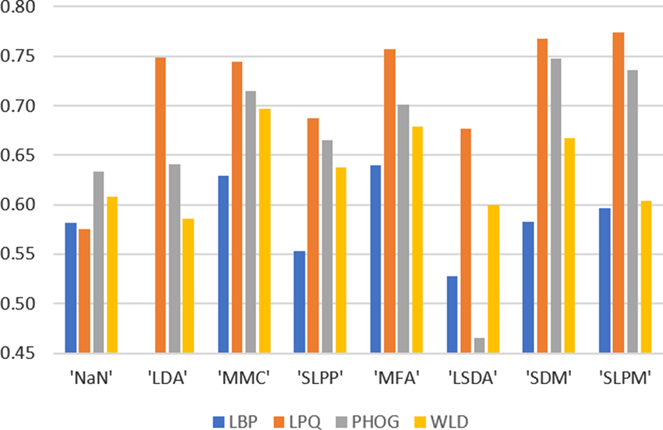
Fig. 5. Recognition rates of the different subspace methods, with different local descriptors, based on a combined dataset of BAUM-2, CK+, JAFFE, and TFEID.
Figure 6 shows the recognition rates of SLPM on COMB4, with the dimensionality of the subspace varied. The results show that SLPM has converged to its highest recognition rate, when the dimensionality is lower than 10. In other words, our method is still very effective even at a low dimensionality. Based on these results, we set the subspace dimensionality at $11$ in the rest of the experiments.
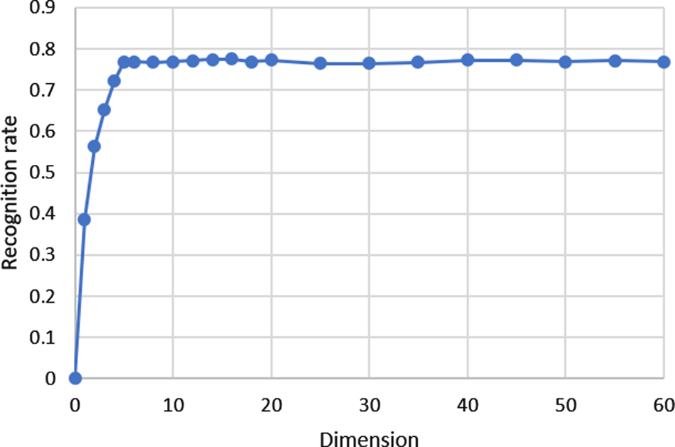
Fig. 6. Recognition rates of our proposed method in terms of different dimensions.
To investigate the effect of the use of images of expression with low intensities, several experiments have been conducted on the CK+ database. As shown in Table 7, the recognition rate is the highest when $\xi =0.9$ . Tables 8 and 9 show the recognition rates of the three subspace-learning methods, MFA, SDM, and SLPM, as well as SLPM, using feature generation with different $\theta _{exp}$
 and $\theta _{ne}$
 values, with the LPQ descriptor, on the four different databases using the nearest neighbor classifier and SVM classifier, respectively. It can be found that SLPM achieves the best classification performance again, when compared to the other methods. The classification performance is further improved by up to 2%, when feature generation is employed. Furthermore, as observed in Tables 8 and 9, the nearest neighbor classifier outperforms the SVM classifier in most of the databases. Finally, additional experiments were conducted to validate the efficiency of the proposed subspace learning methods. Table 10 tabulates the runtimes in milliseconds for each of the subspace learning methods. We can see that SLPM is twice as fast as MFA, which solves the generalized eigenvalue problem instead of calculating eigenvalue decomposition like SLPM. SDM is much slower than MFA and SLPM.
Table 7. Comparison (%) of recognition rates obtained by using low-intensity images with different $\xi$ values on the CK+ database, using the LPQ feature
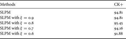
Table 8. Comparison (%) of subspace learning methods on different datasets, with the LPQ descriptor being used with the nearest neighbor classifier
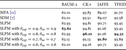
The best results are highlighted in bold.
Table 9. Comparison (%) of subspace learning methods on different datasets, with the LPQ descriptor being used with the SVM classifier

The best results are highlighted in bold.
Table 10. Comparison of the runtimes (in ms) required by the different subspace learning methods (MFA, SDM, and SLPM) on different datasets, with the LPQ descriptor used

The best results are highlighted in bold.
2) Evaluation on SLP-CNN
Comparison with state-of-the-art methods:
We first evaluate SLP-CNN by comparing it with other state-of-the-art deep subspace-learning methods. Specifically, we compare the proposed SLP loss with the other regularizers, including the Center loss [Reference Li and Deng28], the Island loss [Reference Zhao, Liu, Xiao, Lun and Lam26], and the LP loss [Reference Cai, Meng, Khan, Li, O'Reilly and Tong27]. The results are summarized in Table 11, in which the reference model, i.e. Base-CNN, is trained under the standard softmax loss. It can be observed that SLP-CNN consistently outperforms Base-CNN on the four selected databases, which demonstrates that the SLP loss can effectively enhance the discriminative power of the learned features. Compared with the other deep subspace learning regularizers, SLP-CNN surpasses the Center loss and the LP loss by about 2 and 0.5% on the four databases, respectively. This is because the Center and the LP regularizers only penalize the intra-class distance, while the SLP loss considers both the intra-class and the inter-class variations. However, SLP-CNN performs slightly worse than the Island regularizer. The Island loss characterizes the class spread across the whole dataset, while the SLP loss mainly focuses on the local neighborhoods. Therefore, as introduced in Section II.B), the Island loss learns more discriminative features, while the SLP loss can enhance the model generalization. We will further validate this point in the following sections. To better illustrate the performance of the deep subspace regularizers, we visualize the learned deep features of the CK+ testing images. The results are presented in Fig. 7. We adopt t-SNE [Reference Chang and Lin66] to show the 2000-dimensional deep features. It is obvious from the figure that the subspace-learning methods can force the samples with the same expression closer to each other in the latent space, which shows the effectiveness of subspace learning in enhancing the feature discriminative power.
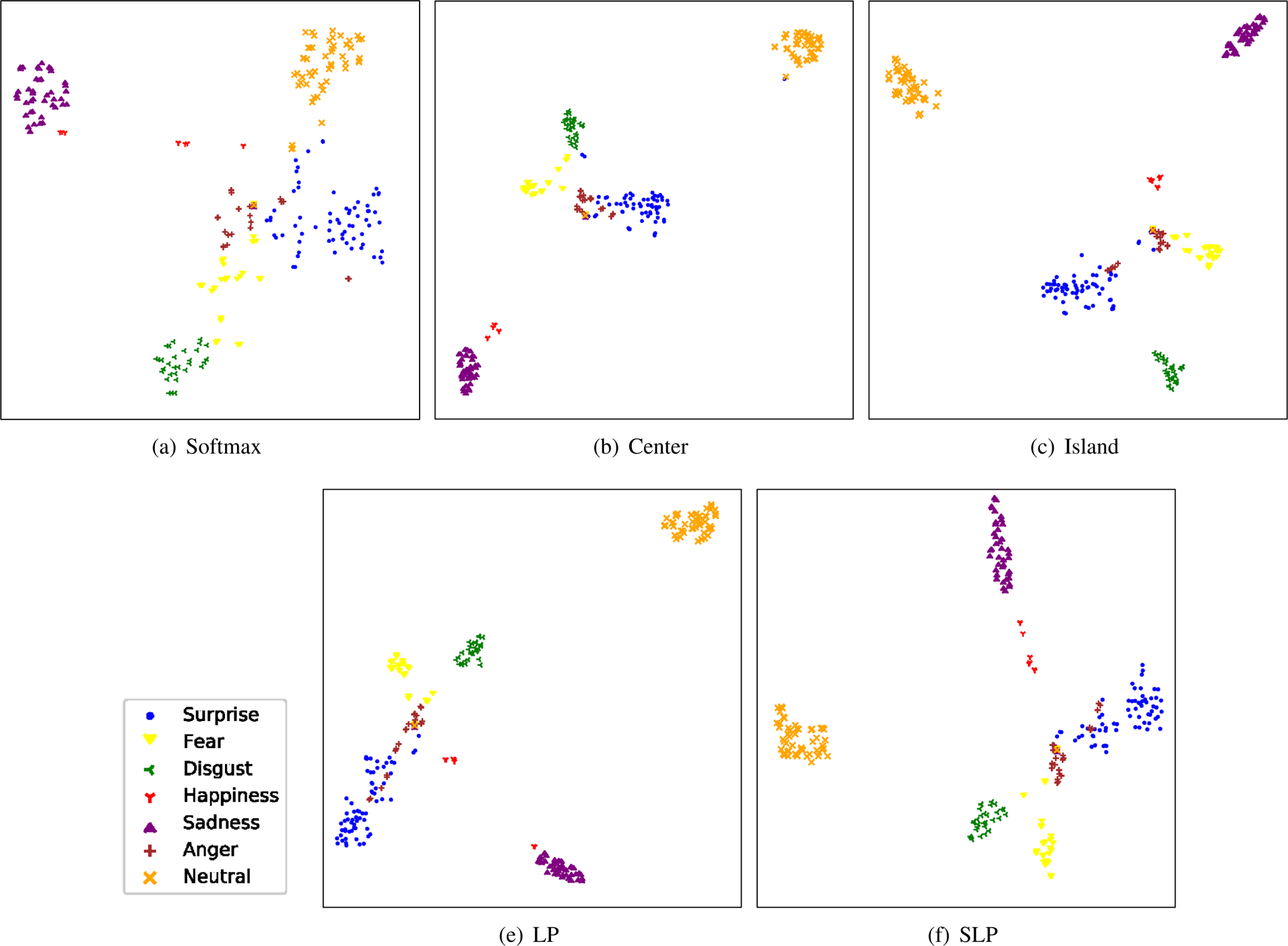
Fig. 7. Visualization of the deeply learned features extracted from the samples of one testing fold in CK+, based on the different methods. (a) Softmax. (b) Center. (c) Island. (d) LP. (e) SLP.
Table 11. Comparison in terms of the recognition rates (%) of the deep subspace-learning methods on different datasets

The best results are highlighted in bold.
Generalization test:
To show the generalization ability of the proposed algorithm, we further conduct the generalization test on SLP-CNN. Specifically, we pretrain the CNN model on the RAF-DB database, and directly employ it to extract features from the images in the four selected databases without fine-tuning. Thus, this is a cross-database evaluation. We also compare the deep subspace-learning methods with other FER algorithms that train and test on the same databases. In other words, we evaluate and compare the deep subspace-learning methods in a more challenging condition. The results are tabulated in Table 12.
Table 12. Generalization test (%) on the different deep subspace regularizers

The deep subspace-learning methods are pretrained on RAF-DB [Reference Cai, Meng, Khan, Li, O'Reilly and Tong27] without further fine-tuning the CNN feature extractors on the target databases. The best results are highlighted in bold.
It can be seen that those deep subspace models, without fine-tuning their feature extraction CNNs, still generalize well on the target datasets. More importantly, the locality-preserving strategy, i.e. the LP and SLP losses, can obtain better generalization ability than the center-based methods, i.e. the Center loss and the Island loss, as the LP and SLP CNNs consistently outperform the Center and Island CNNs on the four target databases. Compared with the other FER methods that train and test on the same domain, the proposed SLP-CNN can produce comparable or even higher recognition accuracy, which demonstrates its effectiveness when facing cross-domain samples in real-world scenarios.
Hyperparameters’ sensitivity analysis: We investigate the sensitivity of the hyperparameters $k$ , $\lambda$
 , and $\beta$
 in equations (43) and (44), which significantly affect the trade-off performance. We first fix $\lambda = 0.1$
 and $\beta =0.5$
 , and explore the effect of $k$
 , which controls the number of nearest-neighbor samples used to compute the SLP loss in a mini batch. Figure 8 reports the results of the recognition accuracy on the four databases, as well as the averaged accuracy over the four databases, in terms of different values of the different hyperparameters. We can observe from Fig. 8(a) that the optimal $k$
 appears at around 20. Similarly, we explore the model sensitivity to $\lambda$
 and $\beta$
 , and present the results in Figs 8(b) and 8(c), respectively. Based on the results, we obtain the settings for the hyperparameters as we introduced in Section V.B), i.e. $k = 20$
 , $\lambda = 0.1$
 , and $\beta = 0.5$
 .
.

Fig. 8. Sensitivity analysis on the hyperparameters in the proposed SLP loss. (a) Effect of $k$ . (b) Effect of $\lambda$
 . (c) Effect of $\beta$
 .
.
VI. CONCLUSION
In this paper, we have given an overview of subspace analysis methods, and extended them to deep learning. We have proposed a subspace-learning method, named SLPM, which uses the neighborhood and class information to construct a projection matrix for mapping high-dimensional data to a meaningful low-dimensional subspace. We further reformulate the SLPM algorithm, and employ it as an additional regularization term for training a DCNN, named SLP-CNN, to enhance the discriminative power and generalization of the learned deep features. The difference between the within-class and between-class matrices is used to define the objective function, rather than the Fisher criteria, in order to avoid the singularity problem. Furthermore, a parameter $\beta$ is added to control the within-class spread, so that the overfitting problem can be solved. The robustness and the generalizability of SLPM and SLP-CNN have been analyzed on four different databases, using four different state-of-the-art descriptors and two different classifiers, and SLPM has been compared with other subspace-learning methods. Moreover, we have proposed using the features of low-intensity expression images to learn a better manifold for each expression class. By taking advantage of domain-specific knowledge, we have proposed two methods of generating new low-intensity features in the subspace. Our experiment results have shown that SLPM outperforms the other subspace-learning methods, and is a good alternative to performing dimensionality reduction on high-dimensional datasets. Our experiment results have also shown that the proposed feature-generation method can further increase the recognition rates.
Acknowledgement
The research described in this paper was supported by the GRF Grant PolyU 15217719 (project code: Q73V) of the Hong Kong Research Grants Council.
Cigdem Turan received her Ph.D. degree from the Department of Electronic and Information Engineering from the Hong Kong Polytechnic University in 2018. Her research interests include affective computing, facial behavior understanding, and responsible artificial intelligence. She is currently a postdoctoral researcher at TU Darmstadt, Germany.
Rui Zhao received his B.Sc. degree in electrical engineering from Xi'an Jiaotong University, China, in 2015, and his M.Sc. degree in electrical and electronic engineering from Imperial College London, UK, in 2017. He is currently a Ph.D. candidate in the Department of Electronic and Information Engineering, The Hong Kong Polytechnic University. His research interests include image processing, computer vision, and facial expression recognition.
Kin-Man Lam received the Associateship in electronic engineering from The Hong Kong Polytechnic University (formerly called Hong Kong Polytechnic) in 1986, his M.Sc. degree in communication engineering from the Department of Electrical Engineering, Imperial College, in 1987, and his Ph.D. degree from the Department of Electrical Engineering, The University of Sydney, in 1996. From 1990 to 1993, he was a Lecturer with the Department of Electronic Engineering, The Hong Kong Polytechnic University, where he joined the Department of Electronic and Information Engineering, as an Assistant Professor in October 1996, became an Associate Professor in 1999, and has been a Professor since 2010.
He was the Director-Student Services and the Director-Membership Services of the IEEE Signal Processing Society between 2012 and 2014, and between 2015 and 2017, respectively. He was an Associate Editor of IEEE Transactions on Image Processing between 2009 and 2014, and Digital Signal Processing between 2014 and 2018. He was also an Editor of HKIE Transactions between 2013 and 2018, and an Area Editor of the IEEE Signal Processing Magazine between 2015 and 2017. Currently, he is the VP-Publications of the Asia-Pacific Signal and Information Processing Association (APSIPA). Prof. Lam serves as an Associate Editor of APSIPA Transactions on Signal and Information Processing and EURASIP International Journal on Image and Video Processing. His current research interests include human face recognition, image and video processing, and computer vision.
Xiangjian He received his Ph.D. degree in computer science from the University of Technology Sydney (UTS), Australia, in 1999. He is currently a Full Professor and the Director of the Computer Vision and Pattern Recognition Laboratory, Global Big Data Technologies Centre, UTS.


 Open access