


I. INTRODUCTION
Hyperspectral imaging sensors are able to capture affluent spectral information across continuous narrow bands. Where the detailed spectral information makes it possible to accurately discriminate materials of interest. Moreover, [Reference Fauvel, Tarabalka, Benediktsson, Chanussot and Tilton1–Reference Zhang, Li, Jia, Gao and Peng4] indicate the fine spatial resolution of the sensors enables the analysis of small spatial structures in the image. Therefore, the rich spatial and spectral characteristics bring wide applications of hyperspectral image (HSI), one of the most popular research directions is the supervised HSI classification.
Extreme learning machine (ELM) has been widely used in supervised HSI classification [Reference Mahesh, Maxwell and Warner5] due to its high efficiency and fast learning speed. ELM [Reference Huang, Zhou and Ding6–Reference Huang, Zhu and Siew8] is a single hidden layer feed-forward neural network with the input weights and biases randomly generated without tedious and time-consuming parameter iterative tuning. Therefore, it maintains the advantage of remarkable training efficiency.
In order to improve the classification accuracy of ELM, the kernel function is used into the ELM model by replacing the activation function, which is termed as kernel ELM (KELM) [Reference Huang, Ding and Zhou9]. The advantages of the KELM function in this algorithm are that the kernel functions used in this algorithm do not need to satisfy Mercer's theorem, and it can also overcome the shortage of random initialization about the input weights and biases, specifically, KELM is robust to the parameters learning [Reference Liu, Wu, Wei, Xiao and Sun10]. It is well known that both of the Gaussian radial basis function (RBF) kernel and composite kernel (CK) [Reference Mahesh, Maxwell and Warner5] applied on KELM have achieved promising classification performance in HSI classification [Reference Mahesh, Maxwell and Warner5, Reference Huang, Zhou and Ding11]. However, the RBF [Reference Ring and Eskofier12] only describes the spectral similarity of the pixels without considering the spatial similarity between the neighbor pixels, and the CK by combining spatial and spectral information that also has its limitations. The [Reference Liu, Wu, Xiao and Yang13] suggested a suitable kernel should learn all high-order similarities between neighboring samples directly, and then reflect the data lie in complex manifolds. Keeping these points in view, in this paper, an efficient KELM algorithm is proposed, which integrates spectral-spatial information by mean filtering (MF) kernel for supervised HSI classification. MF kernel not only computes the spectral similarity but also considers the spatial similarity by averaging the spatial neighboring pixels of the central pixel. Furthermore, we observe that the KELM with MF kernel shows superior performance, and significantly reduces the computational complexity compared with other methods [Reference Camps-Valls, Gomez-Chova, Muñoz Maré, Vila-Francés and Calpe-Maravilla14, Reference Shen, Xu and Li15] simultaneously.
Nevertheless, considering that in the situation of limited training samples, the classification result of MF based on KLEM is very noisy, where the existence of noise in HSI not only degrades the image quality but also reduces the performance. Therefore, it is very critical to propose an effective preprocessing algorithm for HSI noise reduction. The given neighborhood spectral bands always have highly similar spatial and structural characteristics in the context of the HSI. To date, a number of theories have proposed to improve HSI classification performance by taking into spatial and spectral information. Literature [Reference Bau, Sarkar and Healey16] introduced 3D Gabor filters to extract spectral-spatial information from HSI data, and these filters can be used to generate a set of features that captures specific orientation, scale, and wavelength-dependent properties of an HSI region. In [Reference Lu and Li17], Lu and Li presented a gradient-guided sparse representation method by jointly sparse-coding the similar image patches in neighborhood spectral bands of the HSI. In order to improve the classification performance, a novel multiple kernel learning (MKL) algorithm is introduced by integrating multiple types (i.e. multistructure morphological profiles (MPs), multiattribute MPs) of spectral-spatial features with the guidance of an ideal kernel [Reference Gao and Peng18]. What is more, in [Reference Gu, Liu and Jia19], Gu et al. proposed a multistructure-element non-linear MKL, in which the multiple structure elements are employed to generate extended MPs to present spatial-spectral information. Li et al. integrated EMAPs with spectral information to formulate the CK for HSI classification [Reference Li, Reddy Marpu, Plaza, Bioucas-Dias and Benediktsson20]. In [Reference Peng and Rao21], the bilateral filtering exploited on each band-subset to incorporate the spectral signature in the spatial neighborhood. The above methods demonstrate the efficiency to incorporate the spectral and spatial features instead of one single feature. Therefore, in this paper, we utilize the bilateral filtering on the spectral-adaptive band-subsets to exploit their spectral-spatial information. Due to the fact that the high structural similarity spectral bands have continuous spectral characteristics in each band subset, then, the spectral-adaptive band-subsets partition [Reference Lu and Li17] is introduced to gather the highly similar spectral and discard the weak similar ones. The traditional filtering enforces closeness by weighting the pixel values with coefficients that decrease with distance named domain filter. However, in [Reference Tomasi and Manduchi22], noise values that corrupt these nearby pixels are mutually less correlated than the signal values, so noise is averaged away while signal is preserved. It also defined a non-linear range filtering that depends on image intensity or color to average image values with weights that decay with dissimilarity, then, it combines domain filtering with range filtering and denotes it as bilateral filtering, the bilateral filtering smooths each band-subset while preserves the edge information of it. Therewith, we merge the band-subsets together and form a new 3D data cube, where the newly formed cube serves as the input of the MF-KELM classifier.
To tackle the above issues, this paper makes two contributions, summarized as follows:
(1) The proposed MF-KELM method applies the MF kernel to replace the ordinary kernel with the consideration of the underlying data spatial structure as well as the spectral structure.
(2) The proposed Bilateral MF-KELM method, which combines the bilateral filtering and MF-KELM, utilizes the bilateral filtering preprocessing on each spectral-adaptive band-subset in terms of smoothing the image and with the edge information preserved.
The rest of the paper is organized as follows. In Section II, we introduce the MF-KELM classifier for the supervised HSI classification. Part A is a detailed description of the KELM model. Part B is the introduction of the MF kernel. Part C introduces a preprocessing method named bilateral filtering on spectral-adaptive band-subsets. Section III is the experiments and analysis, where we use our statics to prove the efficiency of our proposed method, and compare with some state-of-the-art HSI classification methods based on KELM. Section IV gives a summary of our work.
II. HYPERSPECTRAL IMAGE CLASSIFICATION BASED ON MEAN FILTERING KERNEL EXTREME LEARNING MACHINE
A) Kernel extreme learning machine
ELM [Reference Huang, Ding and Zhou9] is a random generation single-hidden layer feed-forward neural network. KELM is the evolution of ELM, which utilizes the mapping kernel function to replace the hidden layer of ELM. It shows a better performance compared with other methods.
Given N different training samples$\{\textbf{x}_i, {\boldsymbol{z}} _i\} _{i = 1}^N$ , where ${\textbf{x}_i} = \left[ {{x_{i1}},{x_{i2}}, \ldots ,{x_{iD}}} \right] \in {{\mathbb R}^D}$
 , D stands for the number of the spectral bands or dimensionality of the HSI, L is the number of the classes, N represents the number of training samples. The row vector zi = [z i1, …z ik…, z iL] ∈ ℝL determines which class the sample belongs to, we define z ik ∈ {0, 1} and 1 ≤ k ≤ L. If z ik = 1 and any other elements of zi are zero, the sample belongs to the kth class. The output function of the ELM having P hidden neurons defined as follows:
where G(·) represents a non-linear activation function (e.g. RBF), $\boldsymbol{\omega} _j\in {\mathbb R}^D$ is the input weight vector connecting the jth hidden neuron and input neurons, $\boldsymbol{\upbeta} _j\in {\mathbb R}^L$
 is the output weight vector connecting thejth hidden neuron and the output neurons, and b j is the bias of the jth hidden neuron. $\boldsymbol{\upomega} _j\cdot \textbf{x}_i$
 denotes the inner product of $\boldsymbol{\upomega} _j$
 and $\textbf{x}_i$
 . With N samples, equation (1) can be briefly written as


where
Equation (2) can be written as

where $\textbf{H}^\dagger$ is the Moore–Penrose generalized inverse of $\textbf{H}$
 . It can be transformed into the form like $\textbf{H}^\dagger = \textbf{H}^T(\textbf{H}\textbf{H}^T)^{-1}$
 . In order to achieve more stability and generalized inverse classification result, a positive value ρ −1 is added to the diagonal elements of $\textbf{H}\textbf{H}^T$
 . Therefore, the output function of ELM classifier is expressed as follows
where Z ∈ ℝN×L is the training samples label set, similar to SVM, ELM can be generalized to kernel ELM using a kernel trick. The activation function can be replaced by a kernel function; the output function of KELM is expressed as below
where $\textbf{K}_{MF} = [K _{MF}(\textbf{x}_q,\textbf{x}_t)]_{q,t = 1}^N$ , $\textbf{K}_{(\textbf{x}_i)MF}{\rm =} [K _{MF}(\textbf{x}_i,\textbf{x}_1), \ldots,\,K _{MF}(\textbf{x}_i,\textbf{x}_N)]$
 .
.
Note that the label of the test sample is determined by the index of the output node with the largest value. The traditional RBF kernel function is replaced by MF kernel in KELM, and we observe an excellent generation result by doing this.
B) Hyperspectral image classification based on mean filtering kernel extreme learning machine
Although the RBF kernel used in KELM has achieved promising classification performance, it does not consider the underlying data structure of HSI. In order to reflect data relations in a kernel, we adopt the MF kernel [Reference Huang, Ding and Zhou9] and incorporate it into the KELM, and the MF kernel computes the mean value of the spatial neighboring pixels in the kernel space to estimate the central pixel.
Given $\textbf{x}^m\in \Omega ^*$ , m = 1, 2, …, ω 2, and Ω* represents the spatial window, ω is the size of the window, and $\textbf{x}$
 is the center pixel. Let us denote $\phi (\textbf{x}^m)$
 as the image of $\textbf{x}^m$
 under the map ϕ. Then, the MF can be represented as follows
In order to describe the similarity between different pixels, we define the function like
Algorithm 1 MF-KELM
Input: the training samples set $\textbf{X}=[{\bf x}_{1},{\bf x}_{2},\ldots,{\bf x}_N]$ , the test samples set ${\bf Y}{\rm = [}{\bf y}_1, {\bf y}_2,\ldots, {\bf y}_{\rm M}{\rm ]}$
 , window size ω, a positive value ρ, number of classes L.
1. Compute the kernel K pq pixel by pixel in training samples based on equation (7). Then the kernel matrix of training samples $\textbf{K}_{MF}\in {\mathbb R}^{N \times N}$
 consists of all K pq, p = 1, …, N, q = 1, …, N.
2. Compute the kernel K sr pixel by pixel among all samples based on equation (7). Then the kernel matrix $\textbf{K}_{MF}^* \in {\mathbb R}^{M \times N}$
of test samples consists of all $\textbf{K}_{sr}$, r = 1, …, N, s = 1, …, M.3. Calculate the output of test samples $\textbf{Y}$
based on equation (5).4. According to the output of step 3 to achieve the classification prediction: $label(\textbf{y}) = \mathop {\arg} \limits_{t = 1, \ldots, L} \max\, f_t$
.


Output: the estimated label of $\textbf{Y}$ .
.
Where $\textbf{x}_i$ and $\textbf{x}_j$
 represent the two different pixels, respectively.
Algorithm 1 describes the combination of the MF and KELM methods, and we named it MF-KELM.
Image denoising is an image preprocessing work, which has been widely used in the field of HSI processing and has shown a good performance. The following part C is the introduction of bilateral filtering for HSI denoising based on MF-KELM.
C) Spectral band-subsets-wise Bilateral MF-KELM method
Considering the highly similar structural characteristics of neighborhood spectral bands in HSI, which is urgent to exploit the redundant structural information in terms of a better structure characteristics preservation. In this case, based on the structural similarity index metric [Reference Wang, Bovik, Sheikh and Simoncelli23], the spectral-adaptive band-subsets partition [Reference Lu and Li17] method is introduced as follow.
Let I = [I1, I2, …, ID]T represents an HSI cube, where Ii ∈ ℝP×Q is i th band of HSI. Then, we measure the structural similarity between spectral bands Ii and Ii+1 as shown in the following:
where $\mu _{\textbf{I}_i}(\mu _{\textbf{I}_{i + 1}})$ and $\sigma _{\textbf{I} _i}(\sigma _{\textbf{I} _{i + 1}})$
 represent the mean value and the standard deviation of Ii(Ii+1), respectively, here, C 1 and C 2 are constants. When applying equation (8) on adjacent spectral bands, a correlation curve C would generate, where C(i) = SSIM(Ii, Ii+1). Shen et al. [Reference Shen, Xu and Li15] suggest the continuous spectral bands with high structural similarity correspond to relatively stable trend, while obvious drops existing in curve C demonstrate the adjacent spectral bands have much lower structural similarity. Thus, we according to the detection of sharp drops in C to achieve the band-subset partition. Let us define the band-subset as S q, where S q contains B q spectral bands with the size of P × Q.
The bilateral filtering [Reference Tomasi and Manduchi22] defined as the combination of the range and domain filtering, which combines the nearby image values in a non-linear way, and preserves image features with a smooth image while preserving edges. Since the homogeneous regions are commonly contained by HSI, [Reference Shen, Xu and Li15] argues that for each pixel in a band-subset S q, its neighboring pixels will likely share similar spectral characteristics or have the same class membership. Furthermore, the bilateral filtering, which has the ability to influence both the spatial distance and spectral dissimilarity relative to the center pixel, need to extend the general form to the vector form [Reference Peng and Rao21]. We denote S q(a, b) as a pixel of S q, where a and b are the spatial positions of S q, we adopt the same bilateral filtering definition as provided in [Reference Tomasi and Manduchi22]:
where S q(x, y) stands for the neighboring pixel of S q(a, b) within a spatial search window. A a × b matrix neighborhood Ω(a, b) is centered on the target pixel. The weight w(x,y; a, b) can be calculated as

σ r and σ d are the filter parameters and adaptive corresponding to different S q.
After exploiting the spectral-spatial average information of each band-subset S q via bilateral filtering, we merge all the band-subsets into a new three-dimensional data cube, and the cube will act as robust spectral signatures for the input of MF-KELM classifier to predict the final classification results. Figure 1 shows the flowchart of the proposed Bilateral MF-KELM method. Algorithm 2 is the complete description of Bilateral MF-KELM.
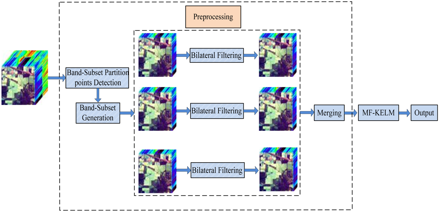
Fig. 1. The flowchart of the proposed Bilateral MF-KELM method.
III. EXPERIMENTS AND ANALYSIS
In this section, we use the Indian Pines dataset to evaluate the performance of the proposed method. Indian pines dataset was collected by the AVIRIS sensor over North western Indiana, and it is an agriculture/forestry landscape with spectrally similar classes and high in-class spectral variability. Figure 2(a) shows the ground truth of Indian Pines dataset. The size of this image is 145 × 145. A total of 20 water absorption and noisy bands (104–108, 150–163, and 220) were removed from the original 220 bands. It contains 16 classes, and 10% of pixels per class randomly selected as the training dataset. In order to evaluate the extensibility and effectiveness of our proposed Bilateral MF-KELM method, we compare it with KSVM [Reference Gu, Liu and Jia19], KELM [Reference Huang, Ding and Zhou9], CK-KELM, Bilateral-KELM [Reference Shen, Xu and Li15], and MF-KLEM [Reference Liu, Wu, Wei, Xiao and Sun10] on the Indian Pines
Algorithm 2 Bilateral MF-KELM
Input: the HSI data cube I, the training samples set $\textbf{X}=[\textbf{x}_{1},\textbf{x}_{2},\ldots,\textbf{x}_N]$ , the test samples set $\textbf{Y}=[\textbf{y}_1, \textbf{y}_2,\ldots, \textbf{y}_M]$
 , C 1, C 2, window size ω, a positive value ρ, number of classes L.
1. Partition the spectral-adaptive band-subsets of HSI, and apply the bilateral filtering to each band-subset, merge them into a new 3D cube data. The above steps depend on equations (8), (9), and equation (10).
2. According to step 1, the new training set $\textbf{X}^*$
and new test set $\textbf{Y}^*$ are obtained.3. Take $\textbf{X}^*$
and $\textbf{Y}^*$ as the input of algorithm 1, then, get the final classification result of the test dataset $\textbf{Y}^*$.


Output: the estimated label of $\textbf{Y}$ .
.
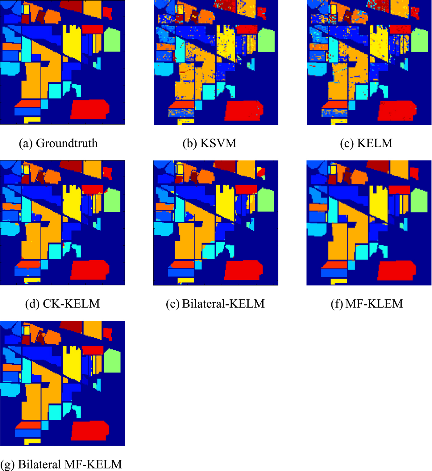
Fig. 2. Indian Pines image. (a) Ground truth; (b) KSVM (OA = 74.21%); (c) KELM (OA = 86.92%); (d) CK-KELM (OA = 94.96%); (e) Bilateral-KELM (OA = 97.29%); (f) MF-KELM (OA = 98.52%); (g) Bilateral MF-KELM (OA = 98.91%).
We adopt the overall accuracy (OA), average accuracy (AA), and the κ coefficient of agreement (k) to measure the classification accuracies, and we also use the Running Time(s) to measure the computational cost, including the Feature Extraction Time(s) and Classification Time(s). All experiments were carried out using MATLAB on an Intel Xeon 2.4.00-GHz machine with 32 GB of RAM.
MF kernel is sensitive to the window size ω. Figure 3 shows the sensitivity of the MF kernel-based method Bilateral MF-KELM to the window size. With the increase of ω, the classification accuracy also increases gradually, but the OA saturates for ω = 11. As ω continues to grow, the decreasing performance suggests that the neighboring relations would be oversmooth. For the preprocessing method, the filter parameters value of σ r and σ d are determined by cross-validation. We set the window size of the bilateral filter that depends on the structure of different scenes to be 9 × 9. In Table 1, the OA of Bilateral MF-KELM method is 98.91%, which is 24.7, 11.99, 3.95, 1.62, and 0.39% higher than the KSVM, KELM, CK-KELM, Bilateral-KELM, and MF-KLEM, respectively. Figures 2(a)–2(g) illustrate the classification maps of the methods mentioned above, it is obvious that the proposed Bilateral MF-KELM method outperforms other compared methods. In addition, the Bilateral MF-KELM mainly contains two steps: the Feature Extraction and the MF-KELM, here, the time complexity of them are O(PQD|Ω(a, b)|2) and O(ω 4DN 2 + N 3), respectively, where |Ω(a, b)| represents the number of pixels in the neighborhood, then, the whole cost is O(PQD|Ω(a, b)|2 + ω 4DN 2 + N 3). The traditional KELM time complexity is O(DN 2 + N 3). It is worth to note that a higher value of ω indicates a higher computation in Bilateral MF-KELM. Therefore, it is suitable to select a much smaller ω value while achieving a good performance.
Table 1. Classification accuracy (%) for Indian Pines image on the test set.
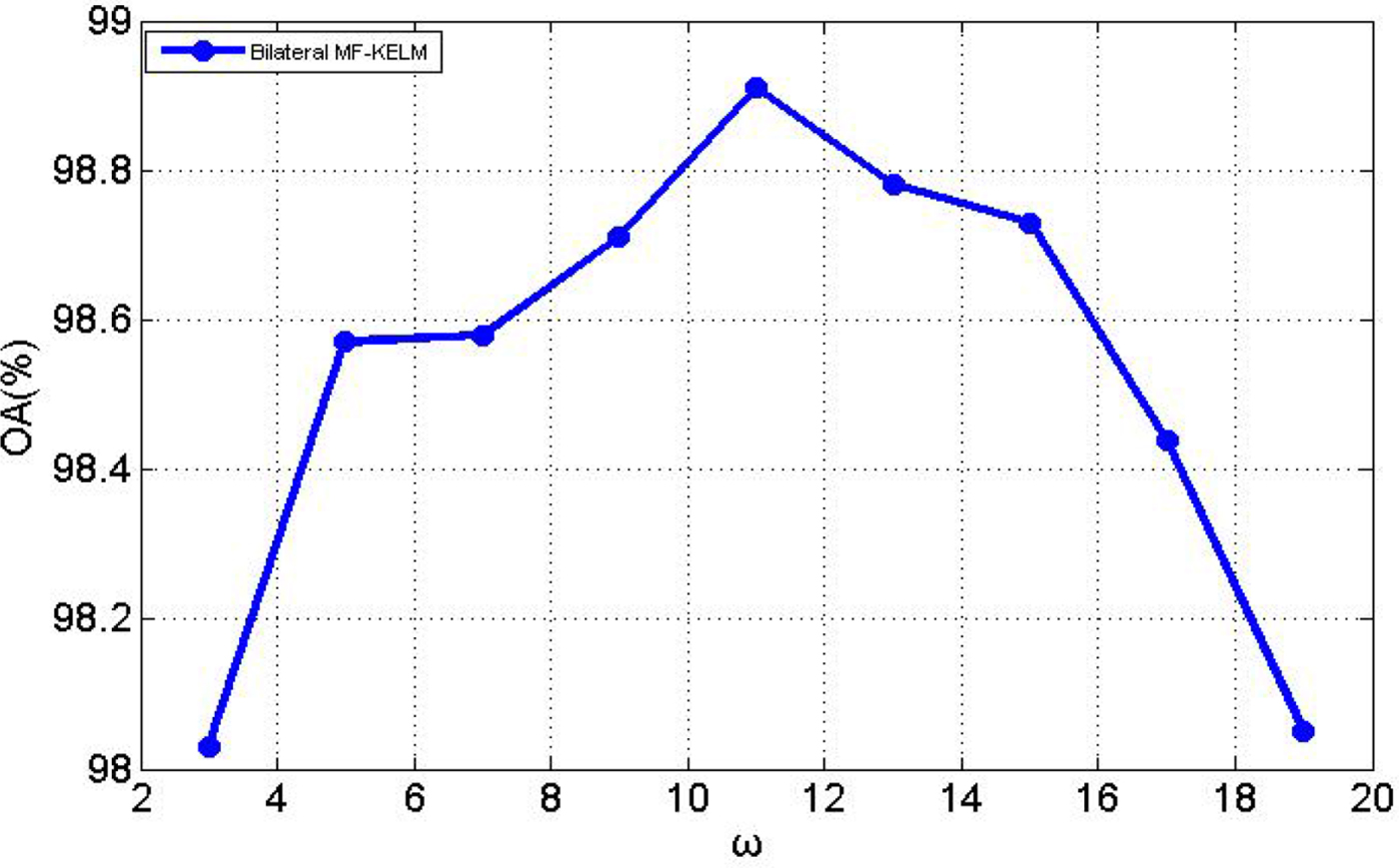
Fig. 3. The classification accuracy for different window sizes ω of Indian Pines in Bilateral MF-KELM method.
IV. CONCLUSION
In this paper, we proposed a novel spectral-spatial Bilateral MF-KELM method of HSI classification, where we incorporate the MF kernel into the KELM model by replacing the original RBF kernel. MF-KELM captures not only the spectral similarity of pixels, but also the spatial similarity of a central pixel by averaging its spatially neighboring pixels in the kernel space. Moreover, in order to overcome the drawback that MF-KELM is unable to eliminate noise effectively, we apply bilateral filtering on each band-subset to reduce the image noise for the HSI preprocessing. By comparing the Bilateral KELM with other different HSI supervised classification methods, obvious visual and numerical merit can be demonstrated in real data experiments.
ACKNOWLEDGEMENTS
This work was supported in part by the National Natural Science Foundation of China under Grant 61471199, Grant 61772274, Grant 61701238, Grant 91538108, Grant 11431015, and Grant 61671243, in part by the Jiangsu Provincial Natural Science Foundation of China under Grant BK20170858, in part by the Fundamental Research Funds for the Central Universities under Grant 30917015104, in part by the China Postdoctoral Science Foundation under Grant 2017M611814. The authors would like to thank Professor Landgrebe from Purdue University for providing the Indian Pines dataset, Professor Gamba from the University of Pavia for providing the University of Pavia dataset, Professor Lin from the National Taiwan University for providing LIBSVM toolbox, and Professor Huang from Nanyang Technological University for providing ELM toolbox.
Wenting Shang received the B.S. degree from Zhengzhou University, Zhengzhou, China, in 2014. She is currently pursuing the Ph.D. degree with the Nanjing University of Science and Technology. Her current research interests include hyperspectral target detection and hyperspectral image classification.
Zebin Wu (M'13–SM'17) was born in Zhejiang, China, in 1981. He received the B.Sc. and Ph.D. degrees in computer science and technology from the Nanjing University of Science and Technology, Nanjing, China, in 2003 and 2007, respectively. In 2016, he joined the Department of Mathematics, University of California at Los Angeles, Los Angeles, CA, USA, as a Visiting Scholar. He was a Visiting Scholar with the Hyperspectral Computing Laboratory, Department of Technology of Computers and Communications, Escuela Politécnica, University of Extremadura, Cáceres, Spain, from 2014 to 2015. He is currently a Professor with the School of Computer Science and Engineering, Nanjing University of Science and Technology. His research interests include hyperspectral image processing, high-performance computing, and computer simulation.
Yang Xu (S'14–M'16) received the B.Sc. degree in applied mathematics and the Ph.D. degree in pattern recognition and intelligence systems from the Nanjing University of Science and Technology (NUST), Nanjing, China, in 2011 and 2016, respectively. He is currently a Lecturer with the School of Computer Science and Engineering, NUST. His research interests include hyperspectral image classification, hyperspectral detection, image processing, and machine learning.
Yan Zhang was born in Jiangsu, China, in 1981. He received the B.Sc. degree from the Suzhou University in 2004.
Zhihui Wei was born in Huaian, China, in 1963. He received the B.Sc. and M.Sc. degrees in applied mathematics and the Ph.D. degree in communication and information system from South East University, Nanjing, China, in 1983, 1986, and 2003, respectively. He is currently a Professor and a Doctoral Supervisor with the Nanjing University of Science and Technology, Nanjing. His research interests include partial differential equations, mathematical image processing, multiscale analysis, sparse representation, and compressive sensing.


 Open access