


I. INTRODUCTION
Speech, the most natural and convenient way for communication, contains abundant information, such as meaning, emotion, and identity. The automatic speaker verification (ASV) is the technique of identifying a person by the provided speech samples. ASV has recently been widely used as a user authentication method. In the meantime, the security of ASV attracts more attention. There are mainly four kinds of attacking methods [Reference Wu, Evans, Kinnunen, Yamagishi, Alegre and Li1]: imitation (i.e. mimicking the voice of the target user), voice conversion (i.e. converting voice of a person into the voice of the target user), speech synthesis (i.e. synthesizing the voice of the target user by the given text), and replay (i.e. replaying a pre-recorded voice of the target user). Among them, replay attacks are easy to implement since they only need to record the voice of the target user and replay the recording with a loudspeaker. Meantime, the quality of recording and playback devices are getting increasingly exquisite, making it difficult to distinguish bonafide attempts from replay attacks. A study has reported that ASV systems are highly vulnerable to replay attacks [Reference Singh, Mishra and Pati2]. To improve the security of ASV, it is important to develop techniques to detect such attacks.
Replay detection is the technique of distinguishing replay speech signals from human (bonafide) speech signals. Three major discrepancies between them are: (1) Flexibility: The content of replay signals is frozen at the time of recording. However, bonafide speeches are dynamically generated by a person at the time of verification. Thus, replay attacks have lesser flexibility than bonafide attempts. Based on this phenomenon, challenge-based approaches [Reference Baloul, Cherrier and Rosenberger3] have been proposed, which require users to respond to a random challenge. (2) Randomness: Due to the randomness of pronunciation, a person can not speak a speech twice in the completely same way. However, the randomness of recording and replay devices is much lesser than the randomness of human pronunciation. Based on this phenomenon, template-matching-based approaches [Reference Paul, Das, Sinha and Prasanna4] have been proposed. Those approaches match a speech signal to template databases to verify whether it is presented earlier or not. (3) Distortion: The replay processes cause distortion, which includes device distortion and environment distortion.
Researchers attempt to detect the distortion. The distortion falls into four categories: (1) Linear distortion: It is related to the flatness of the frequency responses of devices. (2) Nonlinear distortion: It includes harmonic distortion and intermodulation distortion. New frequency components, which do not exist in original signals, will be introduced by nonlinear distortion. (3) Additive noises: It includes the noises caused by physical devices and noises from environments. (4) Reverberations: Since the recordings used for playback also contain reverberations, the reverberations of reverberations will cause distortion in the replay attacks. The distortion mentioned above can be reflected in the cepstral domain. There are several feature sets which are designed in the cepstral domain, such as the constant-Q cepstral coefficients (CQCC) [Reference Todisco, Delgado and Evans5], Mel frequency cepstral coefficients (MFCC), inverse Mel frequency cepstral coefficients (IMFCC) [Reference Li, Chen, Wang and Zheng6], linear prediction cepstral coefficients [Reference Witkowski, Kacprzak, Zelasko, Kowalczyk and Galka7], and rectangular frequency cepstral coefficients (RFCC) [Reference Font, Espín and Cano8]. In addition to magnitude-based features, several phase-based features, such as the modified group delay (MGD) function [Reference Oo, Wang, Phapatanaburi, Iwahashi, Nakagawa and Dang9] and relative phase shift feature [Reference Srinivas and Patil10], have been proposed to detect the distortion in the phase domain.
Apart from these features, classifiers also play an important role in the replay detection task. The Gaussian mixture model (GMM), a traditional statistical model, is popular in this field. However, GMM is a frame-level model. Thus, it can hardly describe the reverberation distortion across multiple frames. Two-dimensional convolutional neural networks (2D-CNN) can model the correlation in both directions, that is, the frequency-axis and time-axis. Thus, they can detect the reverberation effects across frames. Several 2D-CNNs have been used in replay detection, such as the light CNN [Reference Volkova, Andzhukaev, Lavrentyeva, Novoselov and Kozlov11] and ResNet [Reference Chen, Xie, Zhang and Xu12].
In this study, we propose a replay detection method which can detect various replay attacks. The main contributions of our work can be summarized as follows:
Constant-Q transform (CQT)-based modified group delay feature (CQTMGD). To utilize the phase information of the CQT spectrum, we propose a novel MGD feature based on CQT. A spectrogram-based MGD extraction method is also proposed to accelerate the extraction process with the help of a fast algorithm of CQT.
Multi-branch residual convolutional neural network. We propose a novel multi-branch building block for ResNet. The multi-branch structure can enhance generalization and reduce redundancy simultaneously. Moreover, compared with the frame-level GMM, 2D-CNN can better detect time-domain distortion. Thus, it is more suitable for replay detection.
Exploring and analyzing the limitations of models and replay spoofing databases. The class activation mapping (CAM) technique [Reference Zhou, Khosla, Lapedriza, Oliva and Torralba13] was used to visualize the distribution of the attention of the model. We found that the model was focusing on trailing silence and low-frequency bands. Further analysis of trailing silence shows a fake cue in the ASVspoof 2019 dataset. We reestimated the performance after removing the trailing silence in the dataset. The results show that the performance in the original dataset may be over-estimated. Moreover, we analyzed the discriminability of different frequency bands. The results show the differences between the ASVspoof 2019 dataset and the ASVspoof 2017 dataset. It also explains why the CQT-based spectrogram outperformed the discrete Fourier transform-based spectrogram in the ASVspoof 2019 dataset but worse than that in the ASVspoof 2017 dataset.
Compared with the previous work [Reference Cheng, Xu and Zheng14], this work provides more experimental results and in-depth analyses of the proposed method. The results in another widely used replay attack database are provided to evaluate the generalization of the proposed method. The discriminability of different frequency bands was analyzed by using the F-ratio method, and the results explain the performance differences between the two databases. Various silent conditions were further analyzed since the performance may be over-estimated by the trailing silence in the ASVspoof 2019 PA database. Moreover, the distribution of the attention of the model was visualized with three more kinds of input features. A more in-depth analysis of the performance under various recording and replay conditions was performed.
The rest of this paper is organized as follows. In Section II, we review the related works on spoofing detection. Section III describes the proposed CQTMGD, and Section IV describes the multi-branch residual neural network. The experiments are described in Section V, and the results are discussed in Section VI. Further analyses and discussion are presented in Section VII. Our conclusions are presented in Section VIII.
II. RELATED WORK
Feature Engineering. To detect the distortion in replay attacks, various features have been proposed. In [Reference Villalba and Lleida15], Villalba and Lleida proposed four kinds of hand-designed features, namely, the spectral ratio, low frequency ratio, modulation index, and sub-band modulation index. These features capture the distortion caused by far-field recording processes and the non-flat frequency responses of small loudspeakers. Instead of designing features for noticeable distortion, some researchers try to find differences in the entire frequency-domain. The proposed RFCC [Reference Font, Espín and Cano8] and IMFCC [Reference Li, Chen, Wang and Zheng6] use different frequency warping functions from MFCC, while MFCC is widely used in speech processing tasks. This indicates that the importance of different frequency bands in replay detection may differ from traditional speech process tasks. Apart from the traditional Fourier transform, various signal processing methods are also introduced, such as the CQT [Reference Todisco, Delgado and Evans5], single-frequency-filtering technology [Reference Alluri, Achanta, Kadiri, Gangashetty and Vuppala16], and variable-length Teager energy separation algorithm [Reference Patil, Kamble, Patel and Soni17]. However, most of those features only preserve magnitude information and discard phase information, while the phase of signals may also be distorted in the replay processes. To utilize the phase information, Tom et al. [Reference Tom, Jain and Dey18] used the group delay function (GD) in replay detection. Oo et al. [Reference Oo, Wang, Phapatanaburi, Liu, Nakagawa, Iwahashi and Dang19] introduced the relative phase (RP) feature and further extended it in the Mel-scale (Mel-RP) and the gammatone-scale (Gamma-RP). Phapatanaburi et al. [Reference Phapatanaburi, Wang, Nakagawa and Iwahashi20] proposed to extract RP based on the linear prediction analysis (LPA), which extracted RP on the residual signal of LPA.
DNN-based Classifier . Replay detection needs to detect unknown attacks. Thus, many researchers proposed several methods to boost the generalization of DNN. In [Reference Lavrentyeva, Novoselov, Malykh, Kozlov, Kudashev and Shchemelinin21], Lavrentyeva et al. proposed a spoofing detection method based on the light CNN model with the max-feature-map activation. Compared with the traditional CNN, the light CNN has fewer parameters, which can alleviate the overfitting problems in small datasets. In [Reference Adiban, Sameti and Shehnepoor22], an autoencoder was trained to reduce the dimension of CQCC. The bottleneck activations of the autoencoder were fed into a Siamese neural network for classification. Cai et al. [Reference Cai, Wu, Cai and Li23] used data augmentation techniques before training ResNet. Tom et al. [Reference Tom, Jain and Dey18] pre-trained a ResNet model in the ImageNet dataset [Reference Deng, Dong, Socher, Li, Li and Fei-Fei24] and then transformed it for replay detection tasks.
III. CQT-BASED MODIFIED GROUP DELAY FEATURE
In this section, we propose a novel feature for replay detection. The motivation of the novel feature is that the widely used CQCC feature set [Reference Todisco, Delgado and Evans5] discards all the phase information and only preserves the magnitude information of the CQT. Since the distortion of the replay processes is presented not only in the magnitude but also in the phase, the phase information may be helpful for replay detection. To utilize the phase information of CQT, we extract the MGD feature based on CQT to construct what we called the CQTMGD.
A) Group delay function
The GD is defined as the negative derivative of the unwrapped phase spectrum [Reference Murthy and Gadde25]:

where $\omega$ is the frequency variable, $\theta _l(\omega )$
 is the phase spectrum of the signal $x_l(n)$
 , which is the $l$
 -th frame of the entire signal $x(n)$
 . However, it is difficult to estimate the phase spectrum due to the phase wrapping problem. Thus, the GD is usually calculated without the phase spectrum, as follows [Reference Murthy and Gadde25]:

where $Re(\bullet )$ and $Im(\bullet )$
 are the real and imaginary part of a complex variable, respectively. $X_l(\omega )$
 is the spectrum of the signal $x_l(n)$
 and $Y_l(\omega )$
 is the first derivative of $X_l(\omega )$
 , which can also be seen as the spectrum of the signal $nx_l(n)$
 .
.
B) Modified GD
When the energy of a signal (the $|X_l(\omega )|^{2}$ in equation (2)) is close to zero, there will be spiky peaks in the GD. MGD can solve this problem by using the cepstrally smoothed spectrum, called $S_l(\omega )$
 , as the denominator of $\tau _l(\omega )$
 [Reference Murthy and Gadde25]:

where $sign$ is the sign of the original GD, $\gamma$
 and $\alpha$
 are two tunable parameters, varying from 0 to 1.
C) CQT-based MGD feature
The traditional MGD function is extracted with the Fourier transform. The Fourier transform is related to the CQT. Both of them can be seen as a bank of sub-band filters. The main differences between CQT and the Fourier transform is that (1) the center frequencies of CQT filters are geometrically spaced as $f_k = 2^{{k}/{b}} f_0$ , where $f_0$
 is the minimal frequency, and $b$
 is the number of filters per octave, and (2) the bandwidth of each CQT filter is determined by the center frequency as $\delta _k = f_{k+1} - f_k$
 , resulting a constant ratio of center frequency to resolution $Q=({f_k})/({\delta _k})=(2^{{1}/{b}}-1)^{-1}$
 . The CQT is defined as:

where $N_k = Q ({f_s})/({f_k})$ is the length of analysis windows, $f_s$
 is the sample rate of the signal, $W_{N_k}(\bullet )$
 is an arbitrary $N_k$
 -length window function. As a comparison, the definition of the discrete-time Fourier transform is:

It will be found that $X^{cqt}(k) = X^{ft}(({2\pi Q})/({N_k}))$ when $N=N_k$
 . That means CQT can be seen as a type of the Fourier transform with carefully designed varying-length windows and a constant Q-factor, making it reasonable to extract MGD with CQT.
Realizing the relationship between CQT and the Fourier transform, CQT-based MGD can be seen as a bunch of MGD with variable-length frames, i.e.

where $\hat \tau _{l, N_k}(\bullet )$ is the MGD function at the $l$
 -th $N_k$
 -length frame. However, frequency-by-frequency frame-by-frame calculations are time-consuming. To utilize the fast algorithm of CQT [Reference Brown and Puckette26] to accelerate the extraction process, an auxiliary signal $y'(n)$
 is introduced as

For each frame of $y'(n)$ , we have

where T is the hop size between two adjust frames. Thus, we have

Since both $Y'(\omega )$ and $X(\omega )$
 can be calculated by the fast algorithm of CQT, CQT-based MGD can be extracted according to equation (3), as shown in Algorithm 1.
Algorithm 1 CQTMGD ExtractionMethod

IV. MULTI-BRANCH RESIDUAL NEURAL NETWORK
This section describes the details of the multi-branch residual neural network for replay detection. Our hypothesis is that, different from the widely used GMM, the deep residual convolutional neural network could: (1) bring out the discriminative information hidden in time-frequency representation, and (2) learn the dependencies between frames to better model reverberation effects. Moreover, the multi-branch structure can reduce the redundancy of the network as well as increase the generalization for unknown attacks. The blend of the deep residual convolutional neural network and multi-branch structure is named the ResNeWt network.
A) Residual neural network
Residual neural network (ResNet) is widely used in image recognition fields and also explored in the replay detection task [Reference Chen, Xie, Zhang and Xu12]. It eases the optimizing of a deep network by using residual mapping instead of direct mapping. Formally, it tries to learn a residual mapping function $F(x)$ instead of learning the desired underlying mapping $H(x)$
 directly, where $H(x) = F(x)+x$
 . This overcomes the performance degradation when plain CNNs going deeper.
ResNet is constructed by stacking building blocks. In [Reference He, Zhang, Ren and Sun27], two different kinds of building blocks are proposed for ResNet, that is, the basic building block and bottleneck block. The basic block, which consists of two convolutional layers, is used in shallow networks, such as ResNet-18 and ResNet-34. The bottleneck block, which consists of three convolutional layers, is used in deep networks, such as ResNet-50.
B) Multi-branch ResNet
In this paper, a multi-branch building block is proposed. The input of the building block will be processed by K independent paths. The output of each path is concatenated to form the final output of the building block. Due to the independence of each path, the depth of each convolutional kernel is decreased. Thus, the model can be compressed by the multi-branch structure. It is important for replay detection because the limited training data may be overfitted easily. The multi-branch building block is defined as:

where $\textbf {Y}$ is the output of the building block, $\textbf {X}$
 is the input tensor, $f_i(\bullet )$
 can be an arbitrary function which splits the input first and then transforms them, $D$
 is the number of transformations, $\mathop {\Xi }$
 is an aggregate function which concatenates a tensor along the channel-axis, defined as:

where $[S^{(i)}_1,\ldots ,S^{(i)}_k]$ is a k-channel tensor.
A residual neural network with the multi-branch building block proposed above is named ResNeWt. The “W” in the name is the concatenation of the two characters “v”. It implies the multi-branch structure which processes input values separately and concatenates the processing results as the output. The proposed ResNeWt-18, which is based on ResNet-18, is shown in Table 1. There are three main differences: (1) the multi-branch structure is used based on the basic block, (2) the number of filters in the building block is doubled, and (3) a dropout layer is added after global average pooling layer. The spectral feature of each utterance is repeated or/and truncated along the time-axis to ensure the shape of inputs is fixed. Then it is fed into the network to determine whether the utterance is genuine or not.
Table 1. The overall architecture of ResNeWt18. The shape of a residual block [Reference He, Zhang, Ren and Sun27] is inside the brackets, and the number of stacked blocks on a stage is outside the brackets. “C=32” means the grouped convolutions [Reference Krizhevsky, Sutskever and Hinton28] with 32 groups. “2-d fc” means a fully connected layer with 2 units.

There are two commonly used multi-branch neural networks, that is, the Inception network [Reference Szegedy, Ioffe, Vanhoucke and Alemi29] and ResNeXt [Reference Xie, Girshick, Dollár, Tu and He30]. The main difference between the proposed multi-branch structure and the Inception network is the structure of branches. In ResNeWt, all the branches follow the same topological structure. While in Inception, they are different. We use the same structure because it eases the hyper-parameter tuning progress. Comparing ResNeWt with the ResNeXt, both follow the split-transform-merge strategy to build a multi-branch structure. The difference is the aggregate function. In the ResNeXt, it uses the sum function. In ResNeWt, it uses the concatenate function. Thus, the building blocks of ResNeXt need to have more than three layers. Otherwise, it should equal to a wide and dense module [Reference Xie, Girshick, Dollár, Tu and He30]. In contrast, our proposed structure can be applied to an arbitrary number of layers. Thus, the two-layer basic block of ResNet can only be used in ResNeWt.
V. EXPERIMENTAL SETUP
A) Database
The ASVspoof 2019 physical access dataset was used for evaluating the proposed system in this paper. Table 2 describes the subset configuration. This dataset is based upon simulated and carefully controlled acoustic and replay configurations for the convenience of analysis. The simulation processes are illustrated in Fig. 1. The VCTK corpusFootnote 1 was used as the source speech data. Bona fide attempts were simulated by passing the source speeches to an environment simulator. Replay spoofing attempts were simulated by passing the source speeches to an environment simulator first (to simulate recording environments), followed by a device simulator (to simulate playback devices), and then another environment simulator (to simulate playback environments). The environment was assumed to be a room simulated by RoomsimoveFootnote 2 with three parameters, that is, the room size $S$ , reverberation time $RT$
 , and the distance from the talker to the microphone $D$
 . The effects of devices were represented by a quality indicator $Q$
 , which was simulated by the generalized polynomial Hammerstein model and the synchronized sweptsine toolFootnote 3.
Table 2. A summary of the ASVspoof 2019 physical access dataset [31].
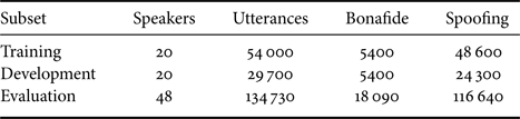

Fig. 1. An illustration of the simulation processes in the ASVspoof 2019 physical access dataset (adapted from [31]).
B) System description
This subsection provides the detailed description of the implemented system.
(1) Feature Extraction: Two categories of feature sets, namely, magnitude-based and phase-based features, were extracted using STFT and CQT. For magnitude-based features, we extracted the STFT-based log power magnitude spectrogram (Spectrogram), Mel scale filter banks (MelFbanks), and CQT-based log power magnitude spectrogram (CQTgram). For phase-based features, we extracted the MGD feature and the proposed CQT-based MGD (CQTMGD) feature. Spectrogram and MelFbanks were extracted with Hamming window, 50 ms frame length, 32 ms frameshift, and 1024 FFT points. A total of 128 Mel filter banks were extracted in MelFbanks. The MGD feature was extracted with 50 ms frame length, 25 ms frameshift, Hamming window, 1024 FFT points, $\alpha =0.6$ , and $\gamma =0.3$
 . The CQTgram and CQTMGD features were extracted with 32 ms frameshift, Hanning window, 11 octaves, and 48 bins per octave. For CQTMGD, we set $\alpha =0.35$
 and $\gamma =0.3$
 . All the features were truncated along the time-axis to preserve exactly 256 frames. The short speeches were extended by repeating itself. Finally, all the inputs were resized to $512\times 256$
 by the bilinear interpolation.
2) Training Setup: ResNeWt was optimized by the Adam algorithm with $10^{-3.75}$ as the learning rate, and the batch size was 16. The training process was stopped after 50 epochs. The loss function was the binary cross-entropy between predictions and targets. The dropout ratio was set to 0.5. The output of the “bonafide” node in the last full connection layer was obtained as the decision score (before the softmax function). The Pytorch toolkit [Reference Paszke, Gross, Chintala, Chanan, Yang, DeVito, Lin, Desmaison, Antiga and Lerer32] was employed to implement the model.
3) Score Fusion: A score-level fusion was performed to combine the models using different features. For simplicity, the ensemble system averaged the output score of all the subsystems. A greedy-based strategy was used in selecting subsystems. First, the best system was chosen. Then, each time, one system was added and the new ensemble system was evaluated in the development set. The best one was selected according to the minimum normalized tandem detection cost function (min-tDCF) (described in Section V.C). The selection process would not stop until the performance no longer improved.
C) Performance evaluation
In the ASVspoof 2019 challenge, the minimum normalized tandem detection cost function (min-tDCF) [31, Reference Kinnunen, Lee, Delgado, Evans, Todisco, Sahidullah, Yamagishi and Reynolds33] was used as the primary metric, which can be calculated as:

where $P_\text {miss}^{\text {cm}}(s)$ and $P_\text {fa}^{\text {cm}}(s)$
 are, respectively, the miss rate and false alarm rate of a countermeasure (CM) system at threshold $s$
 ; $\beta$
 is a cost which depends on the min-tDCF parameters and ASV errors ($\beta \approx 2.0514$
 in the ASVspoof 2019 physical access development set with the ASV scores provided by the organizers of the challenge [31]).
The equal error rate (EER) [31] was also used as the secondary metric.
VI. EXPERIMENTAL RESULTS
A) Comparison of different features
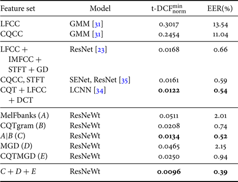
Table 3 depicts a quantitative comparison of different features. Among all the magnitude-based features, CQTgram achieved the lowest EER and almost the lowest min-tDCF. The concatenation of CQTgram and MelFbanks improved the min-tDCF slightly, increasing the EER in the meantime. However, as shown in Fig. 2, the output of CQTgram-based (B) and concatenated feature-based (C) systems were highly correlated. Thus, CQTgram may be the key contributor in the concatenated feature. For the phase-based features, CQTMGD outperformed MGD, which should be attributed to CQT. It indicates that CQT outperformed the Fourier transform in this dataset/task. Finally, score-level fusion achieved further improvements, indicating the complementarity between magnitude and phase, as well as between CQT and the Fourier transform.
Table 3. Performance in the ASVspoof 2019 physical access development set with different features using ResNeWt18 as the classifier.

aA|B: Concatenating the feature set A and B along the frequency-axis with the shape of $656 \times 256 (656 = 528\hbox{(CQTgram)} + 128\hbox{(MelFBanks)})$ .
.
bC+D+E: The fusion (score averaging) of subsystems.

Fig. 2. The correlation between the decision score of the systems using different features in the ASVspoof 2019 physical access development set. A|B is the concatenating of feature A and B along the frequency-axis.
B) Comparison with related models
Table 4 shows the performance achieved by different classifiers in the development set. ResNeWt18 outperformed ResNet18 on the three types of features. ResNeWt34 outperformed ResNet34 on two types of features (CQTgram and CQTGMD). The similar results were achieved for ResNeWt50 and ResNet50. Those results indicate the effectiveness of ResNeWt. However, when comparing ResNeWt50 with ResNeXt50, we found ResNeXt50 achieved better performance. Since the multi-branch structure of ResNeXt cannot be applied to two-layer building blocks, ResNeWt is a good supplement in this field. By comparing the models which use the different numbers of layers, it can be found that the shallow model worked better than the deep model. Based on the results, we chose to use the ResNeWt18 model as the classifier in the rest of the paper.
Table 4. Performance (EER%) in the ASVspoof 2019 physical access development set with different models.

C) Comparison with relevant systems
Table 5 compares the performance of our proposal to other relevant systems. Our proposed system outperformed the baseline systems, as well as other top-performing systems. In particular, the system that used the concatenating of CQTgram and MelFbanks feature as inputs already outperformed other top-performing fusion systems. Compared with the best baseline system, our best fusion system yielded 96.1% and 96.5% relative error reduction on min-tDCF and EER, respectively. Also, it achieved 21.3% and 27.8% relative error reduction on min-tDCF and EER, respectively, compared with the fusion system proposed in [Reference Lavrentyeva, Novoselov, Tseren, Volkova, Gorlanov and Kozlov34].
Table 5. Comparison with relevant systems in the ASVspoof 2019 physical access evaluation set.
D) Performance in ASVspoof 2017 V2
To explore the generalization of the proposed system, we further evaluated it in the ASVspoof 2017 V2 dataset. Due to the limited amount of the training data in the ASVspoof 2017 V2 dataset, the training progress was stopped after 25 epochs. Both the training and development set in the ASVspoof 2017 V2 dataset was used for training.
The experimental results are shown in Table 6. Firstly, both MGD and CQTMGD performed worse than the baseline systems, but the fusion of them outperformed the best baseline system. It shows that both feature sets are informative but not informative enough for replay detection. Secondly, the best single system outperformed the baseline systems, which shows the generalization of the proposed method. Thirdly, the fusion of the four feature sets further improved the performance, which shows the complementarity between those feature sets. Fourthly, overall performance was much worse than the performance reported in the ASVspoof 2019 dataset, which indicates that the real-scene replay data are more challenging than the simulated replay data. Lastly, the Spectrogram feature set outperformed the CQTgram feature set, and MGD outperformed CQTMGD. Those observations may indicate that the Fourier transform outperforms CQT in this dataset. This finding goes against the findings in the ASVspoof 2019 dataset (in Section VI.A). We will analyze it in the discussion section.
Table 6. Comparison with relevant systems in the ASVspoof 2017 V2 evaluation set.

VII. DISCUSSION
A) Contribution analysis
This subsection analyzes the contribution of different components to reveal the causes of the huge performance improvement of the proposed system compared with the baseline systems. As shown in Table 7, there was a dramatic performance improvement when ResNet replaces GMM, and a further improvement was achieved when CQTgram replaces the hand-crafted CQCC feature. This implies that the main contribution of improvement comes from superior modeling capabilities of ResNet, and the use of the low-level feature allows it to exert its modeling capabilities better. Moreover, the proposed ResNeWt achieved about 0.6–4.1% further relative error reduction, compared with ResNet. The fusion of various kinds of magnitude-based and phase-based features further improved performance.
Table 7. Contribution analysis in the ASVspoof 2019 physical access development set comparing with the best baseline system.

B) Conditions analysis
The performance pooled by each simulation factor is shown in Tables 8 and 9. Overall, it was more challenging to distinguish bonafide attempts from replay attack attempts when the room becomes larger. A similar phenomenon was observed when the talker-to-ASV distance, attacker-to-talker distance, and T60 decrease. This phenomenon is related to reverberation distortion. To be more exact, it is related to the reverberation of reverberation (RoR) that is introduced in the playback process. T60 controls the duration of reverberation. Thus, larger T60 will cause more severe reverberation distortion, and that is easier to detect. The room size affects the interval between reflected sounds. Thus, a smaller room causes denser reflected sounds, which can also be seen as a more severe reverberation distortion when T60 is fixed. Recordings captured closer to a microphone are expected to have higher signal-to-reverberation ratio. For devices, as expected, high-quality devices are more difficult to be detected than low-quality devices.
Table 8. Performance (EER%) analysis in the ASVspoof 2019 physical access evaluation dataset pooled by environment configurations.
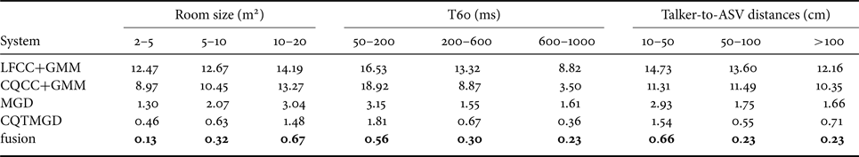
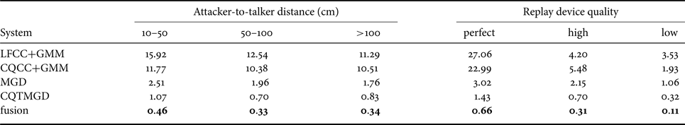
Table 9. Performance (EER%) analysis in the ASVspoof 2019 physical access evaluation dataset pooled by replay configurations.
Different systems perform differently. We found that the frame-level GMM was also sensitive to the reverberation distortion. It is because that the longest interval between two adjacent reflected sounds is about $\sqrt {20}/340 \approx 18.6\,\textrm {ms}$ , which is less than the length of frames. Thus, reverberation distortion is also presented at the frame-level.
Comparing the best GMM system with the best ResNeWt system on the room-size factor, the relative error reduction of GMM from the large-size room to middle-size room was $(13.27-10.45)/13.27 = 21.3\%$ , which is less than the $(0.67-0.32)/0.67 = 52.2\%$
 of ResNeWt. The similar observation was obtained on comparing the middle-size room to the small-size room ($(10.45-8.97)/10.45=14.2\%$
 for GMM and $(0.32-0.13)/0.32=59.4\%$
 for ResNeWt). It shows that ResNeWt was more sensitive to the room-size factor. This is because that the 2D convolution kernel of CNN can capture the correlation along both the frequency-axis and time-axis. Thus, CNN can learn to estimate some factors related to the room size (maybe the interval of reflected sounds). Since RoR will cause a different pattern of the interval of reflected sounds, those estimated factors are distinguishable from bonafide attempts to replay attacks. However, GMM cannot capture this information. Meantime, the relative error reduction on the T60 factor was similar for both GMM and ResNeWt. For the replay device quality, GMM was hard to detect perfect-quality devices, while ResNeWt did much better. It shows the capability of ResNeWt on digging out unobvious discriminative information.
One phenomenon was out of our expectations. The quality of recordings should be improved when the talker-to-ASV distance decreases. Thus, it should be good for replay detection. However, as shown in Table 9, the actual performance degraded. We further analyzed this phenomenon and the results are shown in Table 10. Spoofing attempts became more difficult to detect when the loudspeakers for replay attack get closer to the ASV microphone. However, it seemed to be beneficial for replay detection when real users go far from the ASV microphone, no matter how attackers place the loudspeakers. The reason for this needs further study.
Table 10. Performance (EER%) analysis of the best ResNeWt system in the ASVspoof 2019 physical access evolution dataset pooled by talker-to-ASV distance.

C) Attention analysis
To better understand how the model works, we further visualized the distribution of the attention of the model by the CAM technique [Reference Zhou, Khosla, Lapedriza, Oliva and Torralba13]. In binary classification, the evidence that proves an input signal falling to one category in the meantime indicates the absence of the signal in another category. As we only concerned about the positive evidence, all the negative value in CAM was set to zero.
Figure 3 demonstrates the visualization of attention distributions. There were two apparent patterns. Firstly, the model concentrated on low frequencies (the green solid line box in Fig. 3). It indicates the importance of low-frequency bands. This could explain why CQT worked better than Fourier transform. Since the frequency resolution of CQT in low frequencies is much higher than the Fourier transform, such low frequencies can be hardly distinguished in the Fourier transform-based spectrogram. Also, we should notice that this phenomenon is different from the conclusion found in the ASVspoof 2017 challenge, where the high-frequency bands are more important [Reference Witkowski, Kacprzak, Zelasko, Kowalczyk and Galka7]. This will be further analyzed in the following discussion.

Fig. 3. The attention distribution of the ResNeWt model using the class activation mapping technique [Reference Zhou, Khosla, Lapedriza, Oliva and Torralba13] for the spoofing category. Each row represents an input feature set of the ResNeWt model. Each column represents a randomly selected audio sample from the ASVspoof 2019 physical access development dataset. The filename of each sample is shown on the top of the column. The first two columns (on the left side) are genuine attempts, the last two columns (on the right side) are replay attacks. The green box shows that the models are paying much attention to the lower-frequency range. Best view in color.
Secondly, the model paid much attention to trailing silence, indicating that there is some discriminative information in the silent signal.
D) Trailing silence analysis
To further explore the effect of silence, this subsection analyzes the silence which appears at the end of the speech. The silence discussed here is not the zero values only, but all the low-energy parts. Specifically, since there is no noise in the simulated data, all the non-voice parts of speech are the silence. The energy-based voice activation detection method [Reference Tanyer and Özer37] was used to distinguish the silence from speeches. Figure 4 shows the distribution of the duration of the trailing silence under various T60 conditions. It is shown that when the T60 increases, the duration of the trailing silence becomes longer. This is because that the long-tail silence was mainly caused by the reverberation. Due to the reverberation of reverberation (RoR), spoofing attempts contain longer trailing silence than bonafide attempts.
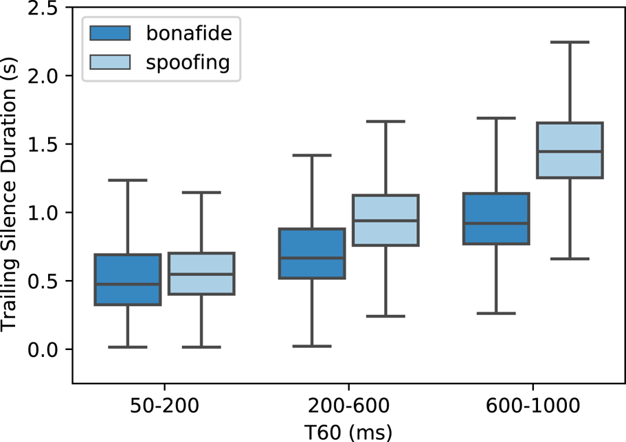
Fig. 4. The distribution of the duration of the trailing silence along with various T60. All the outliers are hidden for clarity.
Suppose the model uses the duration of the trailing silence as a clue to distinguish replay attacks from bonafide attempts. In this case, it can be easily fooled by adding or removing the silence at the end of the signal. Thus, we retrained the model on original recordings (with the silence) but removed the trailing silence during the test phase. The performance of all the models was decreased dramatically, as shown in Table 11 (condition “O - R”). It shows that the model did use the fake clue so that the performance may be overestimated. Those observations agree with the previous work [Reference Chettri, Stoller, Morfi, Ramírez, Benetos and Sturm38] which also found that the performance was over-estimated due to the trailing silence.
Table 11. Results of trailing silence analysis in the ASVspoof 2019 physical access development set. The condition “O” means that the dataset is original, and the condition “R” means that the trailing silence is removed. The condition “X - Y” means the model is trained under condition “X” and tested under condition “Y”. The number on the left of the arrow indicates the performance in the original dataset (i.e. on condition “O - O”).

To prevent the models from using the information on the trailing silence, we removed the trailing silence in the training set and retrained the models. As shown in Table 11 (condition “R - R”), the models worked again, however, with some degradation on performance. Moreover, when the models were trained without the trailing silence and tested with the trailing silence kept, another degradation was observed on all the models except for the CQCC-GMM baseline. This shows that the neural network may be more sensitive to the mismatch between the training and test data. However, this can be easily solved by removing all the silence during the test phase. Overall, the performance of all the proposed models was much better than the baseline system. It demonstrates the capability of the proposed systems.
E) Frequency importance analysis
Previous studies [Reference Tak, Patino, Nautsch, Evans and Todisco39] have reported the different importance of different frequency bands in the anti-spoofing task. In this study, we used the Fisher's ratio (F-ratio) [Reference Wolf40] approach to investigate the discriminability of different frequency bands in the replay attack scenario. F-ratio is defined as the ratio of between-class distance and within-class variance, which can measure linear discriminability between two classes. This is formulated as follows:

where $C_{bonafide}$ and $C_{spoofing}$
 represent two classes, $\mu _i$
 is the mean of class $i$
 , and $\sigma _i$
 is the intra-class variance of class $i$
 .
.
F-ratio for different frequency bands was calculated in the following steps. Firstly, for each speech sample, a spectrogram was extracted by the short-time Fourier transform. Then, the frequency axis of the spectrogram was linearly divided into 50 frequency bands. Finally, the F-ratio values for each frequency band were calculated based on the means and variances of the samples from two classes.
Figure 5 shows the F-ratio values over different frequency bands in two datasets. For the ASVspoof 2019 dataset, the very-low-frequency bands were more discriminable than others. This may be an explanation for the previous finding in Section VII.C that the networks paid more attention to the low-frequency bands. For the ASVspoof 2017 dataset, many researchers have reported that high-frequency bands were more important in replay detection [Reference Li, Chen, Wang and Zheng6, Reference Witkowski, Kacprzak, Zelasko, Kowalczyk and Galka7]. However, the analysis here shows that both the very-low-frequency bands and very-high-frequency bands were discriminable. The reason for this may be related to the different bandwidths of two frequency bands. The bandwidth of discriminable bands in high frequencies is much wider than the discriminable bands in low frequencies. Thus, the wider frequency bands may contain more discriminative information. Moreover, the wider frequency bands are more likely to be found by researchers, and the narrower may be overlooked. For example, a previous study [Reference Li, Chen, Wang and Zheng6] also used the F-ratio method for analysis. However, the number of sub-bands used for analysis was much lesser than this study. Thus, the discriminability of the very-low-frequency bands was not discovered.

Fig. 5. The F-ratio analysis results.
The results here agree with the finding in the study [Reference Lin, Wang and Diqun41], which found that 0–0.5 kHz and 7–8 kHz sub-bands were more discriminative than other frequency bands. Another study [Reference Liu, Wang, Dang, Nakagawa, Guan and Li42], which used the RP for analysis, reported that 0–1 and 4–5 kHz were more informative and discriminative. However, we did not observe the discriminability on 4–5 kHz, which may be because of the different features used for analysis.
Those findings also explain why CQTgram worked better than the Spectrogram feature in the ASVspoof 2019 PA dataset, but not worked well in the ASVspoof 2017 V2 dataset. It is because that the CQTgram feature set can capture more information in low frequencies, however, compress the information in high frequencies. If there is more discriminable information in low-frequency bands than in high-frequency bands (as the ASVspoof 2019 PA dataset), the CQTgram feature set will work better than the Spectrogram feature set. Otherwise, in the ASVspoof 2017 V2 dataset, the Spectrogram feature set captures more information in high-frequency bands than the CQTgram feature set. Thus, the Spectrogram feature set worked better than CQTgram.
We also visualized the F-ratio values for each attack type. The results in the ASVspoof 2017 V2 dataset are shown in Fig. 6. It shows that the discriminability of frequency bands was related to the attack types. Thus, there may need different features for different kinds of attacks. The detailed results in the ASVspoof 2019 dataset are shown in Fig. 7. It shows a high correlation between F-value in low frequencies and the playback device quality. It indicates that the discriminative of low frequencies may be related to the lower cutoff frequency. For the class-C devices, the lower cutoff frequency is larger than 600 Hz. For the class-B devices, the lower cutoff frequency is smaller than 600 Hz. For the class-A devices, the lower cutoff frequency is 0, which means it is ideal. Thus, the class-C device introduces more distortion than the class-A device in very-low-frequency bands.

Fig. 6. The detailed F-ratio analysis results in the ASVspoof 2017 V2 dataset (grouped by replay configurations).

Fig. 7. The detailed F-ratio analysis results in the ASVspoof 2019 physical access dataset (grouped by replay configurations). Attack ID: (replay device quality, attacker-to-talker distance). Environment ID: (room size, T60, talker-to-ASV distance). All the factors fall into three categories (from “a” to “c” or from “A” to “C”).
VIII. CONCLUSION
In this paper, we proposed a novel CQTMGD and a multi-branch residual convolutional network (ResNeWt) to distinguish replay attacks from bonafide attempts. Experimental results in the ASVspoof 2019 physical access dataset clarify that the proposed CQTMGD feature outperformed the traditional MGD feature and ResNeWt also outperformed ResNet.
Compared with the CQCC-GMM baseline, the best fusion system yielded 96.1% and 96.5% relative error reduction on min-tDCF and EER, respectively. Meantime, it outperformed, to the best of our knowledge, all the state-of-the-art systems in the ASVspoof 2019 physical access challenge as well. Further analysis shows that the spoofing samples tend to have a long tail of the silence. To get closer to reality, we cut all the trailing silence and retrained the models. The results show that the performance was decreased but still outperformed the baseline system. The impact of different frequency bands was also analyzed, and we found that both very-low-frequency and very-high-frequency bands contain discriminable information. Moreover, the discriminability of frequency bands is related to replay attack configurations. Thus, different methods may be needed for different types of replay attacks.
Meantime, a counterintuitive phenomenon was found by condition analysis that it seemed to be good for detecting replay attacks when real users are far from the ASV microphone. This needs further analysis in the future.
FINANCIAL SUPPORT
This work was partially supported by the National Basic Research Program (973 Program) of China under Grant No.2013CB329302 and the Tsinghua-d-Ear Joint Laboratory on Voiceprint Processing.
Xingliang Cheng received the B.S. degree in engineering from the Harbin University of Science and Technology, Heilongjiang, China, in 2016. He is a Ph.D. candidate in the Center for Speech and Language Technologies, Beijing National Research Center for Information Science and Technology, Tsinghua University, Beijing, China. He is the recipient of the Best Regular Paper Nomination Award in APSIPA 2019. His research interests include voice biometrics and voice anti-spoofing.
Mingxing Xu received the B.S. degree in computer science and technology and the M.S. and Ph.D. degrees in computer application technology from Tsinghua University, Beijing, China, in 1995, 1999, and 1999, respectively. Since 2004, he has been an Associate Professor at the Department of Computer Science and Technology, Tsinghua University, where his research interests include affective computing, cross-media computing, robust speaker recognition, speech recognition, and human-machine interactive systems.
Thomas Fang Zheng received the B.S. and M.S. degrees in computer science and technology and Ph.D. degree in computer application technology from Tsinghua University, Beijing, China, in 1990, 1992, and 1997, respectively. He is a Professor, Director of the Center for Speech and Language Technologies (CSLT), Executive Deputy Director of Intelligence Science Division, Beijing National Research Center for Information Science and Technology, Tsinghua University. His research and development interests include speech recognition, speaker recognition, emotion recognition, and language processing.


 Open access