


1 Introduction
A popular technique for the numerical solution of many initial-value problems is the family of Runge–Kutta (RK) methods. An historical overview of this approach to solving differential equations is given by Butcher [Reference Butcher7]. Explicit Runge–Kutta (ERK) methods are straightforward to code, because they give explicit formulae for the solution at the next time-step, in terms only of the solution at the current time. The most famous of these is the classical fourth-order, four-stage method in the text by Atkinson [Reference Atkinson3, p. 371]. An improved approach, which still retains the relative simplicity of ERK methods, is provided by the family of Runge–Kutta–Fehlberg methods [Reference Atkinson3, p. 376], in which pairs of RK methods are used together to create explicit formulae that control the growth of numerical error by adaptive time-stepping. A survey of these ideas is presented by Enright et al. [Reference Enright, Higham, Owren and Sharp12], who also discuss concepts such as the detection of stiff zones in the solution and the development of ERK methods specifically for use in systems of second-order equations.
In this current work, we will directly compare the performance of some of the explicit RK methods developed in the last twenty years with the classic fourth-order Runge–Kutta (RK4) method. To make this comparison, we will consider conservative Newtonian orbits as well as a nonconservative relativistic binary system. The aim of this work is to identify which ERK methods are optimal for solving different systems of equations and to discuss any pertinent considerations.
The Newtonian equations for orbital motion of planets in the Solar System are straightforward to write down and lead to a system of conservative second-order differential equations for the positions (and velocities) of each planet. Since this n-body system is nonlinear, it is capable of exhibiting complex behaviours, including resonances, instability, quasi-periodicity and chaos. Long-term simulation of orbital motion therefore requires numerical integration techniques of extremely high accuracy and the question naturally arises as to how far forward in time it is possible to integrate these differential equations, using any quadrature technique, before accumulated numerical error renders the results meaningless.
Anastassi and Simos [Reference Anastassi and Simos2] discuss RK methods for such second-order systems for orbital motions. Because orbital motion is one in which overall energy is conserved, attention has also focussed on symplectic RK methods, and these, too, are surveyed by Enright et al. [Reference Enright, Higham, Owren and Sharp12]. In these techniques, the aim is to preserve, in the numerical approximation, some quantity such as a discrete analogue of energy that should be constant in the exact system of differential equations. This should ensure that orbits remain elliptical, rather than spiralling into the Sun, due to a loss of (discrete) energy in the numerical approximation. An assessment of symplectic methods for Solar System dynamics is presented by Saha and Tremaine [Reference Saha and Tremaine32], and they conclude that these integrators are unquestionably the best available in this context; in this present paper, we will briefly consider the performance of symplectic methods as compared with ERK techniques.
Of course, techniques other than RK methods are also available for the integration of orbital equations. RK methods are single-step integrators, in that the solution at each time-step only depends on conditions at the previous step. Multi-step methods are also possible, however, and can have certain advantages in stability, although now values at each time-step depend on values at the previous k time-steps for a k-step method. Such techniques can be more onerous to code. A mathematical analysis of these methods is presented by Dahlquist [Reference Dahlquist11], and a symmetric multi-step technique has been adapted for orbital systems by Quinlan and Tremaine [Reference Quinlan and Tremaine30]. More recently, Zeebe [Reference Zeebe36] has compared various methods, observing that a Bulirsch–Stoer extrapolative method required vastly more computational time to achieve the same accuracy as a symplectic technique. To improve numerical stability, implicit RK methods have also been developed, in particular, to allow the solution of stiff equations; such systems can occur in orbital-type equations through resonances or relaxation oscillations. In general, however, implicit RK methods require a nonlinear system of algebraic equations to be solved at each time-step, and this could pose considerable difficulty. Consequently, diagonally implicit RK methods have been proposed to make their implementation easier, while nevertheless retaining some of the stability advantages. A review of these techniques has been given by Kennedy and Carpenter [Reference Kennedy and Carpenter24].
The long-term stability of the Solar System is a key question in understanding planetary dynamics and accurate, reliable large-time integrations of the governing equations are usually necessary. Laskar [Reference Laskar26] reported numerical integrations of approximate, averaged equations of Solar System motion, from which he concluded that the Solar System is chaotic. Resonances in the motions of the inner planets made his numerical solutions unreliable at some time beyond 10 mega-years (Myr). Laskar et al. [Reference Laskar, Quinn and Tremaine27] confirmed these results by integrating the equations for the whole Solar System over a 6-Myr time interval, and showed the presence of resonances in the motions of the Earth and Mars. These findings are consistent with a subsequent integration of the Newtonian equations for the Sun and eight planets, carried out by Batygin and Laughlin [Reference Batygin and Laughlin4]. Their results also showed an instability in the motion of Mercury, which eventually destabilizes the Solar System. Olsen et al. [Reference Olsen, Laskar, Kent, Kinney, Reynolds, Sha and Whiteside29] likewise found that long-term numerical solutions were only reliable over an interval of 60 Myr, and that the system becomes chaotic. However, here we are simulating n-body problems to demonstrate accuracy of integrators and so are concerned only with numerical instabilities. We note that stellar system integrations normally use mixed-variable symplectic methods based on the work of Wisdom and Holman [Reference Wisdom and Holman35], which are more efficient in dealing with close encounters of two bodies. We will briefly consider a fourth-order symplectic method, but will not consider the more specialized methods developed for orbital mechanics.
Relativistic orbits may also be considered a type of n-body problem, requiring forward integration to simulate the orbits as they spiral inwards. The field of gravitational wave (GW) astronomy has progressed greatly since the detection of the first merging binary black hole (BBH) system in September 2015 [Reference Abbott1]. The advanced Laser Interferometer Gravitational-wave Observatory (aLIGO) uses a matched-filtering detection algorithm to target a 4-dimensional parameter space describing the most common variants of compact binary sources, that is, those with spin-aligned components on quasi-circular orbits [Reference Gerosa, Kesden, Berti, O’Shaughnessy and Sperhake17, Reference Huerta and Brown19, Reference Rodriguez, Chatterjee and Rasio31]. However, several studies have suggested this algorithm may miss compact binaries formed in dense stellar environments due to their more eccentric orbits [Reference Huerta and Brown19–Reference Huerta21, Reference Klimenko25]. Constructing the template waveforms involves numerically solving the Einstein field equations to describe the inspiral, merger and ringdown. The large (9-dimensional) parameter space and computationally intensive nature of numerical relativity (NR) simulations has led to the development of accurate Keplerian-type parametric solutions including a post-Newtonian (PN) approximation [Reference Hinder, Herrmann, Laguna and Shoemaker18]. The PN approximation invokes a gauge-invariant dimensionless parameter, x, related to the total mass of the binary system and the orbital frequency. The temporal evolution of this parameter is computed using a first-order differential equation that considers the present state of the Keplerian-type orbit and the PN corrections [Reference Huerta21, equation (5)]. The eccentricity, mean anomaly and phase of the orbit are typically computed with this gauge-invariant parameter as a coupled system of ordinary differential equations (ODEs). The waveform for the merger-ringdown, for example, derived using the IRS model introduced by Kelly et al. [Reference Kelly, Baker, Boggs, McWilliams and Centrella23] and calibrated with NR simulations [Reference Huerta21], can be appended to that of the inspiral phase.
Large systems of ODEs may also arise from the numerical solution of partial differential equations (PDEs) in fluid mechanics or combustion theory, for example. Any numerical technique that approximates the spatial derivatives in some manner results in a large system of time-dependent ODEs that must be integrated forward in time. RK methods are often employed for this purpose. There are three broad classes of techniques that are of this type. The first are methods such as finite-element or discontinuous Galerkin methods, in which spatial variations are approximated over collections of small elements of finite size. Examples of these approaches are given in the review by Cockburn and Shu [Reference Cockburn and Shu9]. A second type is related to the method of lines, in which finite differences are used to approximate only the spatial derivatives, so that the PDE is replaced by a system of ODEs at each spatial node point. Verwer [Reference Verwer33] applies this approach to the solution of parabolic PDEs, which arise in diffusion processes, and a somewhat similar approach has been used recently by Zhao et al. [Reference Zhao, Huang and Ruuth38] to solve systems of nonlinear wave equations in conservation form. The third group of techniques are spectral methods, in which the unknown function is expressed as a series of orthogonal functions in space, with time-dependent Fourier coefficients that solve systems of ODEs that must be integrated forward in time. Walters and Forbes [Reference Walters and Forbes34] recently used methods of this type to study Rayleigh–Taylor instabilities in fluid mechanics, in three space variables and using RK methods for the time integration. We do not consider PDEs further in this paper, however, instead focus on ODE systems arising in orbital motions. Our primary interest is ERK methods, since these are the easiest to code, for large systems of ODEs, and so are the first choice in a wide variety of applications. We will consider two types of problems to be solved: n-body Newtonian systems and a two-body relativistic binary orbit. These are areas of current interest and we give a very brief introduction to these topics here.
This present paper is concerned with higher-order ERK methods, which will be examined in the solution of n-body systems, and their practical implementation. These methods are equally applicable to the solution of PDEs as described above, and Forbes et al. [Reference Forbes, Walters and Hocking15] employed a $10$
th-order, 16-stage ERK recently to study a problem in free-surface hydrodynamics.
$10$
th-order, 16-stage ERK recently to study a problem in free-surface hydrodynamics.
In Section 2, we lay out the general structure of ERK methods and identify the particular methods used here. Section 3 presents the n-body equations and our numerical scheme to solve them. We provide modern Fortran code and show the results of tests using methods of various orders. The performance of these methods for Newtonian Solar System orbits is discussed, and in Section 3.4, they are also applied to a two-body post-Newtonian system radiating gravitational waves. A discussion concludes the paper in Section 4.
Throughout this study, we have compared results obtained using double-precision (64-bit floats) and quad-precision (128-bit floats). Many modern compilers allow this choice to be made by means of a single compiler switch, as was the case here, using the open-source compiler, gfortran. We note, however, that calculations using quad-precision floats are implemented via an additional software layer and so perform slower by some orders of magnitude on standard desktop hardware.
2 Explicit Runge–Kutta methods
ERK methods have the property that function values at each new time-step depend only on values at the current time level. This makes these methods fast and particularly simple to code. For clarity, the ERK method is used to solve an initial value problem of the form
 $$ \begin{align*} \frac{d y}{d t}=f(t,y(t)),\quad y(t_0)=y_0, \end{align*} $$
for some known function f, with initial value $y_0$
at known time
$y_0$
at known time $t_0$
. The solution after a small time-step
$t_0$
. The solution after a small time-step $\Delta t$
is given by
$\Delta t$
is given by
 $$ \begin{align*} t_{n+1}&=t_n+\Delta t , \nonumber \\ y_{n+1} &= y_n + \Delta t \sum_{i=1}^p b_i k_i, \end{align*} $$
with
 $$\begin{align*}k_i=f\bigg(t_n+c_i \Delta t,y_n+\Delta t \sum_{j=1}^{i-1} a_{ij}k_j\bigg). \end{align*}$$
The coefficients $a_{ij}, b_i, c_i$
are defined by the particular RK method chosen. The
$a_{ij}, b_i, c_i$
are defined by the particular RK method chosen. The $a_{ij}$
components are a set of coefficients in lower triangular matrix form. For a method of p stages,
$a_{ij}$
components are a set of coefficients in lower triangular matrix form. For a method of p stages, $i=j=p$
, there are a total of
$i=j=p$
, there are a total of $p(\, p-1)/2$
such coefficients, although some of these may be zero. There are p weights,
$p(\, p-1)/2$
such coefficients, although some of these may be zero. There are p weights, $b_j$
. The
$b_j$
. The $c_i$
components are simply the sum of the corresponding row of
$c_i$
components are simply the sum of the corresponding row of $a_{ij}$
components, that is,
$a_{ij}$
components, that is, $c_i=\sum _{j=1}^{i-1}{a_{ij}}$
. Newtonian n-body problems may be classified as autonomous systems, that is, systems in which the derivative function, f, (in this case, acceleration) does not depend on the independent variable (time), but only on the dependent variables (position, velocity). For such systems, the intermediate function evaluations,
$c_i=\sum _{j=1}^{i-1}{a_{ij}}$
. Newtonian n-body problems may be classified as autonomous systems, that is, systems in which the derivative function, f, (in this case, acceleration) does not depend on the independent variable (time), but only on the dependent variables (position, velocity). For such systems, the intermediate function evaluations, $k_i$
, take a slightly simpler form:
$k_i$
, take a slightly simpler form:
 $$ \begin{align*} k_i&=f\bigg(y_n+\Delta t \sum_{j=1}^{i-1} a_{ij}k_j\bigg), \nonumber \end{align*} $$
and the $c_i$
components are not required.
$c_i$
components are not required.
Each ERK method may be characterized by its “Butcher tableau”, being a visual display of these coefficients used for each step of the ERK method. The number p of stages of an RK method is the number of function evaluations performed at every time-step of the integration routine. The order of an RK method is a measure of the accuracy of the method, in terms of powers of the time-step, $\Delta t$
. The “classic” fourth-order method has four stages and is fourth-order accurate in global truncation error (the numerical solution at the final time will vary from the true solution by a factor proportional to
$\Delta t$
. The “classic” fourth-order method has four stages and is fourth-order accurate in global truncation error (the numerical solution at the final time will vary from the true solution by a factor proportional to $\Delta t^4$
). The number of stages required for a given order increases quickly for high-order methods, although the general formula defining the required number of stages for a given order is not known. A method is generally labelled by its order. Thus, the Butcher RK6 method is a sixth-order method, although it requires seven function evaluations (stages) per time-step. The Butcher tableau for a general ERK of p stages is presented in the left panel of Figure 1, and as specific examples, Runge and Kutta’s “classic” RK4 method [Reference Atkinson3, p. 371] is presented in the middle panel and Butcher’s RK6 method [Reference Butcher6] (with his choices of
$\Delta t^4$
). The number of stages required for a given order increases quickly for high-order methods, although the general formula defining the required number of stages for a given order is not known. A method is generally labelled by its order. Thus, the Butcher RK6 method is a sixth-order method, although it requires seven function evaluations (stages) per time-step. The Butcher tableau for a general ERK of p stages is presented in the left panel of Figure 1, and as specific examples, Runge and Kutta’s “classic” RK4 method [Reference Atkinson3, p. 371] is presented in the middle panel and Butcher’s RK6 method [Reference Butcher6] (with his choices of $\lambda =4, \mu =1/3$
, these being additional constraints that are chosen to complete the definition of a particular method) on the right.
$\lambda =4, \mu =1/3$
, these being additional constraints that are chosen to complete the definition of a particular method) on the right.

Figure 1 The Butcher tableau is a standard way of displaying the coefficients for RK methods. For ERK methods, the $a_{ij}$
coefficients are displayed in lower-triangular matrix form, with their row-sums,
$a_{ij}$
coefficients are displayed in lower-triangular matrix form, with their row-sums, $c_i$
, as a column on the left and the integration weights,
$c_i$
, as a column on the left and the integration weights, $b_j$
, as a row underneath. The general form for ERK methods is shown in the left panel, the “classic” RK4 method is in the centre panel and one of Butcher’s RK6 methods is shown in the right panel.
$b_j$
, as a row underneath. The general form for ERK methods is shown in the left panel, the “classic” RK4 method is in the centre panel and one of Butcher’s RK6 methods is shown in the right panel.
In the current paper, we consider RK methods ranging from the classic RK4 method with four stages up to a 35 stage $14$
th-order method. With
$14$
th-order method. With $p=35$
stages, the highest-order method investigated here has
$p=35$
stages, the highest-order method investigated here has $35 \times 34/2=595\ a_{ij}$
coefficients. Regardless of the number of stages and coefficients, the numerical algorithm is the same and will be described in Section 3, along with a small code sample.
$35 \times 34/2=595\ a_{ij}$
coefficients. Regardless of the number of stages and coefficients, the numerical algorithm is the same and will be described in Section 3, along with a small code sample.
Table 1 The seven methods investigated in this work are listed below, showing number of stages and order of accuracy. The number of stages increases rapidly with increasing order of accuracy.

Seven explicit RK methods are considered in this work, which will mostly be referenced by the number of stages they contain. These are listed by the number of stages and order of accuracy of each method in Table 1. We note that several of these methods can be expanded to embed methods of lower or higher order, which allow the use of adaptive stepsize control. We have not investigated the use of adaptive stepsize in the current work, although we note that such methods may be efficient, particularly for high ellipticity orbits where the accelerations and velocities vary greatly throughout the orbital path.
3 The $\boldsymbol {n}$
-body simulations
$\boldsymbol {n}$
-body simulations

A system of three or more bodies interacting under Newtonian gravity has motion of the bodies which is not generally solvable analytically. However, given knowledge of the masses, positions and velocities of all of the bodies (“initial conditions”), these systems may be integrated forward in time to determine positions and velocities at a future time. Such a simulation of Newtonian n-body problems requires the solution of the gravitational equation
 $$ \begin{align*} \ddot{\mathbf{r}_{\mathbf{i}}}=-\sum_{j=1}^n \frac{m_j}{r_{ij}^3} \mathbf{r}_{\mathbf{ij}}: \mathbf{i}\, \neq\, \mathbf{j} , \end{align*} $$
where $\mathbf {r}_{\mathbf{ij}}$
is the position vector from the jth body to the ith body,
$\mathbf {r}_{\mathbf{ij}}$
is the position vector from the jth body to the ith body, $r_{ij}$
is the corresponding distance,
$r_{ij}$
is the corresponding distance, $m_j$
is the mass of the jth body and
$m_j$
is the mass of the jth body and $\ddot {\mathbf {r_{i}}}$
is the acceleration of the ith body, and units have been chosen such that Newton’s constant has value 1. The components in Cartesian co-ordinates have equations:
$\ddot {\mathbf {r_{i}}}$
is the acceleration of the ith body, and units have been chosen such that Newton’s constant has value 1. The components in Cartesian co-ordinates have equations:
 $$ \begin{align*} \ddot{x_{i}}&=-\sum_{j=1}^n \frac{m_j}{r_{ij}^3} (x_i-x_j): i \neq j , \nonumber\\ \ddot{y_{i}}&=-\sum_{j=1}^n \frac{m_j}{r_{ij}^3} (y_i-y_j): i \neq j , \nonumber\\ \ddot{z_{i}}&=-\sum_{j=1}^n \frac{m_j}{r_{ij}^3} (z_i-z_j): i \neq j , \nonumber\\ r_{ij}&=\sqrt{(x_j-x_i)^2+(y_j-y_i)^2+(z_j-z_i)^2}.\nonumber \end{align*} $$
The RK methods integrate first-order equations, so the three second-order Newtonian equations are re-written as six first-order equations:
 $$ \begin{align*} \dot{x_{i}}&=v^{\,x}_{i}, \quad \dot{y_{i}}=v^{\,y}_{i}, \quad \dot{z_{i}}=v^z_{i}, \nonumber\\ \dot{v^{\,x}_{i}}&=-\sum_{j=1}^n \frac{m_j}{r_{ij}^3} (x_i-x_j): i \neq j , \nonumber\\ \dot{v^{\,y}_{i}}&=-\sum_{j=1}^n \frac{m_j}{r_{ij}^3} (y_i-y_j): i \neq j , \nonumber\\ \dot{v^z_{i}}&=-\sum_{j=1}^n \frac{m_j}{r_{ij}^3} (z_i-z_j): i \neq j , \nonumber\\ r_{ij}&=\sqrt{(x_j-x_i)^2+(y_j-y_i)^2+(z_j-z_i)^2},\nonumber \end{align*} $$
where $v^{\,x}_{i}, v^{\,y}_{i}$
and
$v^{\,x}_{i}, v^{\,y}_{i}$
and $v^z_{i}$
are the Cartesian velocity components of the ith body. For a system containing n bodies, this is now a coupled system of
$v^z_{i}$
are the Cartesian velocity components of the ith body. For a system containing n bodies, this is now a coupled system of $6n$
first-order differential equations to be integrated forward in time. Here we first consider some simple two- and three-body systems. These include elliptical orbits and two simple three-body systems, with orbital paths shown in Figure 2, and as described below. These are followed by a nine-body Solar System model, and a relativistic binary black hole inspiral.
$6n$
first-order differential equations to be integrated forward in time. Here we first consider some simple two- and three-body systems. These include elliptical orbits and two simple three-body systems, with orbital paths shown in Figure 2, and as described below. These are followed by a nine-body Solar System model, and a relativistic binary black hole inspiral.
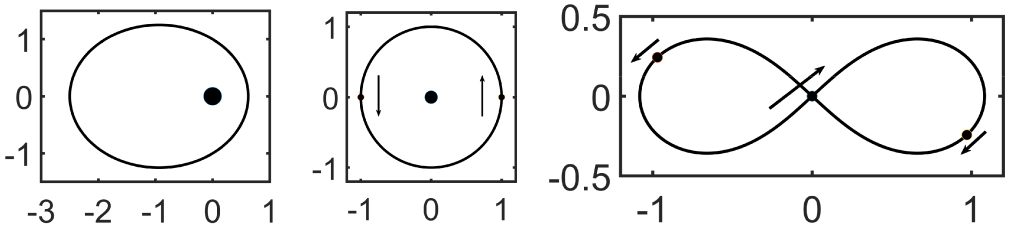
Figure 2 The orbital paths of the two- and three-body simulations, showing the initial locations of the bodies, along with an indication of their initial velocities, represented by the arrows. The left panel shows the simplified two-body orbit, where the mass is all located at the origin and a much lighter body orbits in an elliptical path. The ellipse shown here has eccentricity of $0.6$
. The central panel shows the orbits of two massive bodies orbiting a more massive central body. The right panel shows the path of three equal mass bodies chasing each other around a figure-eight path. Initially, the central body has twice the speed of the other two bodies, but in the opposite direction, so that the system has zero total momentum.
$0.6$
. The central panel shows the orbits of two massive bodies orbiting a more massive central body. The right panel shows the path of three equal mass bodies chasing each other around a figure-eight path. Initially, the central body has twice the speed of the other two bodies, but in the opposite direction, so that the system has zero total momentum.
We found it expedient to load the $a_{ij}$
and
$a_{ij}$
and $b_j$
values from text files at the start of the program. The explicit RK calculation is then written in a general way that works correctly with any number of stages. For illustration, the RK calculation to move the system forward by the small time-step
$b_j$
values from text files at the start of the program. The explicit RK calculation is then written in a general way that works correctly with any number of stages. For illustration, the RK calculation to move the system forward by the small time-step $\Delta t$
is shown in Figure 3, in modern Fortran, for an RK method with number of stages equal to
$\Delta t$
is shown in Figure 3, in modern Fortran, for an RK method with number of stages equal to $rksteps$
. The positions and velocities of all of the bodies in the system are stored in vectors
$rksteps$
. The positions and velocities of all of the bodies in the system are stored in vectors $x,y,z,vx,vy,vz$
. For example,
$x,y,z,vx,vy,vz$
. For example, $x(1)$
is the x-value of the first body, and
$x(1)$
is the x-value of the first body, and $x(n)$
is the x-value of the nth body. The “accel” code is a simple routine that calculates the Newtonian acceleration of each body due to all the other bodies in the system. This routine takes in the arrays containing the position data for all the bodies in the system (in this case,
$x(n)$
is the x-value of the nth body. The “accel” code is a simple routine that calculates the Newtonian acceleration of each body due to all the other bodies in the system. This routine takes in the arrays containing the position data for all the bodies in the system (in this case, $xi,yi,zi$
) and their corresponding masses (
$xi,yi,zi$
) and their corresponding masses ( $masses$
) and the number of bodies in the system (
$masses$
) and the number of bodies in the system ( $n\ masses$
), and returns the component accelerations (
$n\ masses$
), and returns the component accelerations ( $vxk, vyk, vzk$
, that is, the derivatives of the velocity components). These acceleration data are stored in
$vxk, vyk, vzk$
, that is, the derivatives of the velocity components). These acceleration data are stored in $vxk, vyk, vzk$
for each of the stages of the RK routine, and for each body. “Matmul” is the intrinsic Fortran routine for matrix multiplication. The time values after each step of the integration process are stored in the variable t.
$vxk, vyk, vzk$
for each of the stages of the RK routine, and for each body. “Matmul” is the intrinsic Fortran routine for matrix multiplication. The time values after each step of the integration process are stored in the variable t.
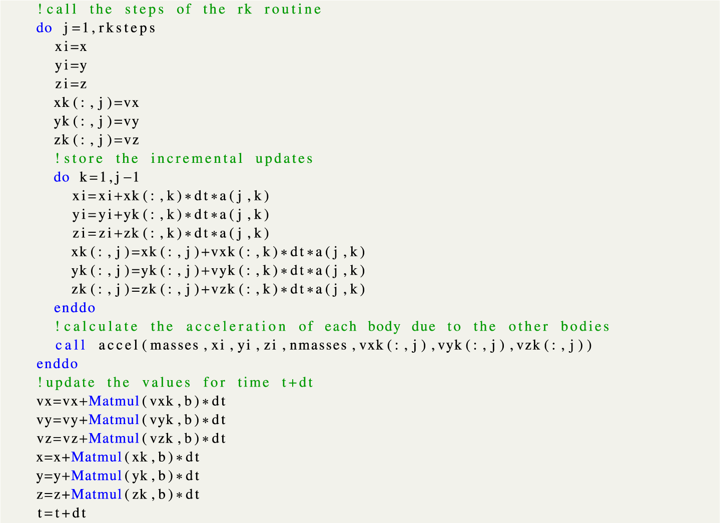
Figure 3 The n-body 3D code to utilize any of the ERK methods, is shown here in modern Fortran. The initial values are loaded into the variables $xi$
etc. Next, the intermediate integration point is determined, based on the
$xi$
etc. Next, the intermediate integration point is determined, based on the $a_{ij}$
values. The accelerations at that point are determined, based on the masses and positions of all the other bodies. Finally, the positions and velocities are updated based on all the integrated values at each stage, weighted by the
$a_{ij}$
values. The accelerations at that point are determined, based on the masses and positions of all the other bodies. Finally, the positions and velocities are updated based on all the integrated values at each stage, weighted by the $b_j$
weights.
$b_j$
weights.
For clarity, the “accel” routine for the n-body simulations is shown in Figure 4, apart from the variable definitions. The term $r2$
is the square of the distance between two bodies, and
$r2$
is the square of the distance between two bodies, and $r3$
is the inverse of the cube of that distance.
$r3$
is the inverse of the cube of that distance.

Figure 4 The code snippet used to update the position of each body. The “cycle” statement skips the calculation where $m=j$
. That is, the body’s acceleration is not affected by its own position and mass.
$m=j$
. That is, the body’s acceleration is not affected by its own position and mass.
The accuracy of any forward-integration scheme, such as the one shown in Figure 3, is dependent on the smallness of the time-step $\Delta t$
. The dependence of accuracy on the stepsize is illustrated in Figure 5. For this illustration, a circular orbit has been numerically integrated using Zhang’s
$\Delta t$
. The dependence of accuracy on the stepsize is illustrated in Figure 5. For this illustration, a circular orbit has been numerically integrated using Zhang’s $10$
th-order 16-stage method [Reference Zhang37] for
$10$
th-order 16-stage method [Reference Zhang37] for $1000$
orbits. The position of the satellite in the final orbit is compared against its analytically determined position. The maximum discrepancy in position in the final orbit is plotted against the stepsize, using
$1000$
orbits. The position of the satellite in the final orbit is compared against its analytically determined position. The maximum discrepancy in position in the final orbit is plotted against the stepsize, using $\log _{10}$
scales. This line has a slope of
$\log _{10}$
scales. This line has a slope of $9.82$
, demonstrating that the method is close to
$9.82$
, demonstrating that the method is close to $10$
th-order accurate (that is,
$10$
th-order accurate (that is, $\Delta err \propto \Delta t ^ {9.82}$
).
$\Delta err \propto \Delta t ^ {9.82}$
).

Figure 5 Display of error level due to different stepsize $\Delta t$
. Both the error and
$\Delta t$
. Both the error and $\Delta t$
are displayed using log scales, which appears as a linear relation, demonstrating the power law dependence of accuracy on
$\Delta t$
are displayed using log scales, which appears as a linear relation, demonstrating the power law dependence of accuracy on $\Delta t$
. This graph compares results at different step-sizes for a simple circular orbit using quad-precision (128-bit floats) integrated by the 16-stage
$\Delta t$
. This graph compares results at different step-sizes for a simple circular orbit using quad-precision (128-bit floats) integrated by the 16-stage $10$
th-order method. The error is relative to the analytically determined position for the final orbit after 1000 orbits.
$10$
th-order method. The error is relative to the analytically determined position for the final orbit after 1000 orbits.
In comparing the various RK methods, the computational time is primarily dependent on the number of function evaluations, being the number of time-steps multiplied by the number of RK stages per time-step. For the remainder of this study, the error will be plotted against the number of function calls.
3.1 Kepler orbits
The best known orbital system is the two-body system, acting under Newtonian gravity. The two bodies follow paths that are conic sections. We consider here a bound orbit (an ellipse), and also further simplify the problem by considering a body at the origin, and an orbiting body of comparably small mass. In this case, the solution consists of no motion of the body at the origin, while the orbiting body follows an elliptical path, with one focus at the origin.
The test system is set up with a body with dimensionless mass $1$
at the origin. A particle of negligible mass orbits in an elliptical path with specific angular momentum
$1$
at the origin. A particle of negligible mass orbits in an elliptical path with specific angular momentum $L=1$
, eccentricity
$L=1$
, eccentricity $\epsilon $
, semi-major axis
$\epsilon $
, semi-major axis $a=L^2/(1-\epsilon ^2)$
. Such an orbit has period
$a=L^2/(1-\epsilon ^2)$
. Such an orbit has period $T=2 \pi a^{3/2}$
. At time
$T=2 \pi a^{3/2}$
. At time $t=0$
, we set
$t=0$
, we set
 $$ \begin{align*}(x,y,z)=(L^2/(1+\epsilon),0,0)\quad \text{and} \quad (\dot x,\dot y,\dot z)=(0,(1+\epsilon)/L,0).\end{align*} $$
These initial conditions describe an ellipse in the x–y plane.
To compare the seven RK methods under consideration, the elliptical system is integrated forward in time for $100$
orbits. The final orbit is compared with the analytical solution at each time-step in the final orbital period. Specifically, the relative error is defined as
$100$
orbits. The final orbit is compared with the analytical solution at each time-step in the final orbital period. Specifically, the relative error is defined as $Err=((x_{rk}-x_{an})^2+(y_{rk}-y_{an})^2)/r_{an}^2$
, where
$Err=((x_{rk}-x_{an})^2+(y_{rk}-y_{an})^2)/r_{an}^2$
, where $x_{an}$
and
$x_{an}$
and $x_{rk}$
are the x-values of position computed with the analytical method and the RK method, respectively, and similarly for y and r. The largest value of this error in the final orbit is plotted for each method for various numbers of evaluation steps per orbit, in Figure 6. The upper panels show the results using double precision (64-bit floats), and the lower panels show the results using quad-precision (128-bit floats).
$x_{rk}$
are the x-values of position computed with the analytical method and the RK method, respectively, and similarly for y and r. The largest value of this error in the final orbit is plotted for each method for various numbers of evaluation steps per orbit, in Figure 6. The upper panels show the results using double precision (64-bit floats), and the lower panels show the results using quad-precision (128-bit floats).

Figure 6 Maximum variation of position for each of the RK methods for elliptical orbits. The eccentricity varies from 0 to 0.9. The legend shows the different RK methods by their number of stages. The x-axis shows the number of function evaluations per orbit. The y-axis shows the variation relative to the analytic value for the final orbit. Both axes use $\log _{10}$
scaling. The upper figures show results using double precision (64-bit floats), the lower using quad-precision (128-bit floats).
$\log _{10}$
scaling. The upper figures show results using double precision (64-bit floats), the lower using quad-precision (128-bit floats).
For the high eccentricity cases, the stepsize has been significantly reduced to handle the rapid motion of the orbiting body whilst near the origin. It may be seen in Figure 6 that the runtime has been increased by a factor of approximately 30 in the $\epsilon =0.9$
case over the
$\epsilon =0.9$
case over the $\epsilon =0.3$
case. It is clear that the efficiency in high eccentricity cases would be increased by the use of an adaptive stepsize method, but this has not been pursued here.
$\epsilon =0.3$
case. It is clear that the efficiency in high eccentricity cases would be increased by the use of an adaptive stepsize method, but this has not been pursued here.
Figure 6 shows the error, on a logarithmic scale, versus the number of function evaluations per orbital period, also on a logarithmic scale. The number of function evaluations is therefore the number of stages of the method multiplied by the number of time-steps per orbit. Thus, at the same number of function evaluations, Zhang’s $10$
th-order 16 stage method has a time-step that is four times as large as that of the four-stage RK4 method. It may be observed that, given a sufficiently small time-step, the higher-order integrators consistently reach the same level of precision for lower computational cost. This is particularly so with the quad-precision models. However, caution should be taken when using large stepsizes, where the
$10$
th-order 16 stage method has a time-step that is four times as large as that of the four-stage RK4 method. It may be observed that, given a sufficiently small time-step, the higher-order integrators consistently reach the same level of precision for lower computational cost. This is particularly so with the quad-precision models. However, caution should be taken when using large stepsizes, where the $12$
th- and
$12$
th- and $14$
th-order integrators, in particular, may perform very badly. It is also apparent that there is a minimum useful stepsize for each method, beyond which there are no further improvements in accuracy. This is seen in the “levelling off” in the double-precision graphs. Once the accuracy of the method is close to the limit of the machine-precision, reducing the stepsize will not help. In fact, it may be seen in Figure 6 that decreasing the stepsize beyond this point, resulting in more function evaluations, actually decreases accuracy slightly due to greater accumulation of “rounding errors”.
$14$
th-order integrators, in particular, may perform very badly. It is also apparent that there is a minimum useful stepsize for each method, beyond which there are no further improvements in accuracy. This is seen in the “levelling off” in the double-precision graphs. Once the accuracy of the method is close to the limit of the machine-precision, reducing the stepsize will not help. In fact, it may be seen in Figure 6 that decreasing the stepsize beyond this point, resulting in more function evaluations, actually decreases accuracy slightly due to greater accumulation of “rounding errors”.
These results suggest that high-accuracy double-precision calculations will be performed accurately with the $10$
th- and
$10$
th- and $12$
th-order integrators, and the classic RK4 is much slower. In the case of quadruple-precision, the
$12$
th-order integrators, and the classic RK4 is much slower. In the case of quadruple-precision, the $12$
th-order method is excellent, and may be a safer method than the
$12$
th-order method is excellent, and may be a safer method than the $14$
th-order, unless very small time-steps are used.
$14$
th-order, unless very small time-steps are used.
A note on symplectic methods: Symplectic methods are suited to conservative systems such as the Newtonian systems we are considering. While a detailed investigation of these methods is beyond the scope of this paper, we did perform some simulations of the Kepler orbit with a fourth-order symplectic integrator (the optimized method of [Reference McLachlan and Atela28]) for an elliptical orbit with eccentricity $0.6$
. The symplectic method is compared with the RK4 and RK6 methods in Figure 7. These three methods were evaluated with respect to the analytically determined elliptical orbit. In every case, the fourth-order symplectic integrator was more efficient than the classic RK4 method, but less efficient than the RK6 method (which is itself usually less efficient than even higher-order methods, as seen in Figure 6). This suggests that at a given order, n-body problems are solved more efficiently with an optimized symplectic integrator, if available. However, for high positional accuracy, the order of the method is more important than whether the method is symplectic or not.
$0.6$
. The symplectic method is compared with the RK4 and RK6 methods in Figure 7. These three methods were evaluated with respect to the analytically determined elliptical orbit. In every case, the fourth-order symplectic integrator was more efficient than the classic RK4 method, but less efficient than the RK6 method (which is itself usually less efficient than even higher-order methods, as seen in Figure 6). This suggests that at a given order, n-body problems are solved more efficiently with an optimized symplectic integrator, if available. However, for high positional accuracy, the order of the method is more important than whether the method is symplectic or not.

Figure 7 Comparison of the fourth-order symplectic method with the four- and seven-stage RK methods. The x-axis shows the total number of function evaluations for an elliptical system with eccentricity of 0.6. The y-axis shows the variation relative to the analytic value for the orbit. Both axes use $log_{10}$
scaling. The upper panel shows results using 64-bit floats, the lower using 128-bit floats.
$log_{10}$
scaling. The upper panel shows results using 64-bit floats, the lower using 128-bit floats.
3.2 Three-body orbits
While there is no solution to the general Newtonian three-body problem, many solutions to particular three-body systems are known. We first consider here a simple three-body system with central body at the origin with dimensionless mass $1$
, orbited by two satellites of mass
$1$
, orbited by two satellites of mass $0.1$
situated on opposite sides of the origin, at radius
$0.1$
situated on opposite sides of the origin, at radius $1$
. These satellites have initial speed
$1$
. These satellites have initial speed $\sqrt {1+0.1/4}$
, as required for a circular orbit. The accuracies of the RK methods against the exact circular orbit are shown in Figure 8, in double- and quad-precision. Even in the double-precision case, it may be seen that the fourth-order method takes approximately 50 times as long to reach the
$\sqrt {1+0.1/4}$
, as required for a circular orbit. The accuracies of the RK methods against the exact circular orbit are shown in Figure 8, in double- and quad-precision. Even in the double-precision case, it may be seen that the fourth-order method takes approximately 50 times as long to reach the $10^{-10}$
accuracy level as the
$10^{-10}$
accuracy level as the $10$
th- and
$10$
th- and $12$
th-order methods, so the savings are not insignificant. For very high accuracy, the
$12$
th-order methods, so the savings are not insignificant. For very high accuracy, the $12$
th- and
$12$
th- and $14$
th-order methods clearly perform better than the lower-order methods in this problem.
$14$
th-order methods clearly perform better than the lower-order methods in this problem.

Figure 8 Maximum variation of position for each of the RK methods for the circular three-body problem. The legend shows the different RK methods by their number of stages. The x-axis shows the number of function evaluations per orbit. The y-axis shows the variation relative to the analytic value for the final orbit. Both axes use $\log _{10}$
scaling. The upper panel shows results using 64-bit floats, the lower using 128-bit floats.
$\log _{10}$
scaling. The upper panel shows results using 64-bit floats, the lower using 128-bit floats.
Another stable three-body system is the remarkable figure-eight system with three equal masses and zero total momentum [Reference Chenciner and Montgomery8]. The three bodies are initially placed co-linearly, as shown in the right panel in Figure 2. The body at the origin has twice the velocity of the other two bodies. This system has a region of stable orbits. The accuracy of the integration methods is tracked by variations in the total momentum of the system (which should remain zero). The accuracy of the RK methods is shown in Figure 9. As with the circular three-body system, the $12$
th- and
$12$
th- and $14$
th-order methods clearly out-perform the other methods in the high-accuracy region, but perform poorly when used with large stepsizes, particularly the
$14$
th-order methods clearly out-perform the other methods in the high-accuracy region, but perform poorly when used with large stepsizes, particularly the $14$
th-order method. In the double-precision case, the fourth-order method is very slow, and even the sixth-order method is significantly slower than the higher-order methods.
$14$
th-order method. In the double-precision case, the fourth-order method is very slow, and even the sixth-order method is significantly slower than the higher-order methods.

Figure 9 Final maximum absolute value of the variation of angular momentum for each of the RK methods for the figure-eight three-body problem. The legend shows the different RK methods by their number of stages. The x-axis shows the number of function evaluations per orbit. The y-axis shows the maximum absolute value of the total angular momentum for the final orbit. Both axes use $log_{10}$
scaling. The upper panel shows results using 64-bit floats, the lower using 128-bit floats.
$log_{10}$
scaling. The upper panel shows results using 64-bit floats, the lower using 128-bit floats.
3.3 Solar System orbits
We now consider the orbits of the nine major bodies in our Solar System (the sun and the eight planets). Initial position and velocity data were obtained from the JPL web interface [22]. The co-ordinate system was then adjusted to place the origin at the barycentre, and the system integrated forward in time. To measure the accuracy of the RK integrators, the z-component of the initial angular momentum was compared with the angular momentum at each time-step in the final (Earth) year of the simulation, and the largest relative error displayed against each RK method for a various number of function evaluations per (Earth) year. For context, the variation of the z-component of momentum for each of the bodies is shown in Figure 10, smoothed for clarity using a 25-year moving average, to remove short-timescale, high-amplitude variabilities. It may be seen that while the total momentum of the system should remain constant, there is significant transfer of momenta between the bodies. This transfer is dominated by Jupiter and Saturn, with a period of just over 50 000 years. There is also a longer envelope visible with a period of approximately 600 000 years. However, for the main purpose of this paper, the concern is with accuracy, which in this case may be assessed by considering the change in total momentum. Total momentum should be conserved, so the best integration methods have the lowest variation. A comparison of the seven RK methods is shown in Figure 11, considering the total change in the z-component of momentum after a period of time. The double-precision model (upper panel) was simulated over a period of 500 000 earth years. Calculations using quad-precision numbers are not directly supported in hardware, resulting in much longer runtimes. To perform comparisons in a reasonable time, the quad-precision runs were conducted over a period of 1000 simulated earth years.

Figure 10 Variation in the z-component of angular momentum for each of the nine Solar System bodies over 500 000 years, smoothed with a 25-year moving average. The variation is dominated by Jupiter (black) and Saturn (red online), exchanging momenta over a 50 000-year period. The total momentum of the system should remain zero.

Figure 11 Final maximum absolute value of the variation in the total system z-component of angular momentum for each of the RK methods for the nine-body Solar System. The legend shows the different RK methods by their number of stages. The x-axis shows the number of function evaluations per orbit. The y-axis shows the maximum absolute value of the total angular momentum for the final orbit. Both axes utilize $\log _{10}$
scaling. The upper panel shows results using double precision (64-bit), the lower using quad-precision (128-bit).
$\log _{10}$
scaling. The upper panel shows results using double precision (64-bit), the lower using quad-precision (128-bit).
The comparison of the RK methods here shows similarities with the two- and three-body systems discussed previously. The higher-order methods generally perform better, reaching higher accuracy for the same computational effort, given a suitably small time-step. Again, caution is advised when using the highest-order method as it may perform worse than the other methods for large time-steps. The $10$
th- and
$10$
th- and $12$
th-order methods perform well consistently, with the
$12$
th-order methods perform well consistently, with the $12$
th-order method clearly outperforming lower-order methods in the quad-precision simulation. The
$12$
th-order method clearly outperforming lower-order methods in the quad-precision simulation. The $14$
th-order method does not appear to be a good choice in the double precision runs, but may outperform all lower-order methods in the quad-precision simulation, given a small enough time-step.
$14$
th-order method does not appear to be a good choice in the double precision runs, but may outperform all lower-order methods in the quad-precision simulation, given a small enough time-step.
3.3.1 Long-time simulations
Over a long period of time, it was found that the simulation fails at some point. Presumably, this is due to accumulation of errors associated with the Runge–Kutta approximation (also known as “truncation errors”). This is demonstrated in Figure 12 by the diverging of the extrema of the angular momenta of the orbiting bodies, occurring at approximately 4.9 million years for a simulation using 85 time-steps per earth year, and at 13.4 million years when using 90. Up until this point, the individual angular momenta show a pattern similar to that seen in Figure 10, oscillating back and forth regularly, but staying between extrema which do not vary. The point in time at which this divergence occurs is strongly dependent on the stepsize ( $\Delta t$
) used. Feagin’s 17-step RK10 method was used for these long-term Solar System simulations. In Figure 13, we show a simulation using 95 time-steps per year (dashed lines), laid over the 90 time-steps simulation (dotted lines), and zoomed in to the time when the divergence occurs. We see that the two simulations are visually indistinguishable until approximately 13.38 million years, at which time the coarser simulation (larger
$\Delta t$
) used. Feagin’s 17-step RK10 method was used for these long-term Solar System simulations. In Figure 13, we show a simulation using 95 time-steps per year (dashed lines), laid over the 90 time-steps simulation (dotted lines), and zoomed in to the time when the divergence occurs. We see that the two simulations are visually indistinguishable until approximately 13.38 million years, at which time the coarser simulation (larger $\Delta t$
) diverges rapidly. In the lower panel, we have added the results from use of the fourth-order symplectic method, using 80 time-steps per year. This method maintains angular momenta terms as well as Feagin’s RK10 method using 95 time-steps per year. As noted earlier, this is the design strength of symplectic methods, but they do not match the accuracy of the higher-order RK methods. That is, symplectic methods maintain the conserved quantities, such as energy and momentum, but this does not guarantee that the bodies will be in the correct position at each time, as was demonstrated by comparison to an analytical model in Figure 7.
$\Delta t$
) diverges rapidly. In the lower panel, we have added the results from use of the fourth-order symplectic method, using 80 time-steps per year. This method maintains angular momenta terms as well as Feagin’s RK10 method using 95 time-steps per year. As noted earlier, this is the design strength of symplectic methods, but they do not match the accuracy of the higher-order RK methods. That is, symplectic methods maintain the conserved quantities, such as energy and momentum, but this does not guarantee that the bodies will be in the correct position at each time, as was demonstrated by comparison to an analytical model in Figure 7.

Figure 12 Variation in z-component of angular momentum for the nine-body Solar System. The upper panel show the results using 85 time-steps per earth year, which become unstable at 4.9 million years. The lower panel used 90 time-steps per year and became unstable at 13.4 million years.

Figure 13 Comparison of the variation in the z-component of angular momentum for the nine-body Solar System using Feagin’s RK10 method. In the upper panel, we have used dotted lines (with squares) and dashed lines (with circles) for 90 or 95 points per year, respectively. It may be seen that the two methods diverge at $1.338\times 10^7$
years. A fourth-order symplectic method has been added in the lower panel, shown with a dash-dot line, with “+” markers. This symplectic simulation used 80 points per year, with four function calls per point. Additional magnification is used in the lower panel. By observing that the “+” and circle markers stay together, it is apparent that the symplectic method maintains the angular momenta terms better than a much slower (90 points per year) RK method.
$1.338\times 10^7$
years. A fourth-order symplectic method has been added in the lower panel, shown with a dash-dot line, with “+” markers. This symplectic simulation used 80 points per year, with four function calls per point. Additional magnification is used in the lower panel. By observing that the “+” and circle markers stay together, it is apparent that the symplectic method maintains the angular momenta terms better than a much slower (90 points per year) RK method.
The time to failure ( $\log _{10}$
scale) is plotted against the number of points per year in Figure 14. This shows a strong power-law correlation between the number of time-steps used and the time at which numerical failure occurs. However several points did not fit this model well, with some failing significantly earlier than expected. We assume that this is due to a particular value of time-step causing a function evaluation at a time when there is higher than normal accelerations, such as a conjunction of planets. This causes a larger truncation error which slowly builds, eventually causing failure of the integration procedure. Perhaps this is an example of a slow-burning numerical instability such as that mentioned in relation to the DuFort–Frankel averaging method by Galloway and Ivers [Reference Galloway and Ivers16]. While caution is indicated, the simulation time is clearly significantly extended by increasing the number of time-steps. The graph in Figure 14 suggests that 120 points per year would be sufficient to allow a simulation up to one billion years. It is possible that adaptive time-stepping methods would avoid this instability, as they do not accept truncation errors larger than a pre-defined value.
$\log _{10}$
scale) is plotted against the number of points per year in Figure 14. This shows a strong power-law correlation between the number of time-steps used and the time at which numerical failure occurs. However several points did not fit this model well, with some failing significantly earlier than expected. We assume that this is due to a particular value of time-step causing a function evaluation at a time when there is higher than normal accelerations, such as a conjunction of planets. This causes a larger truncation error which slowly builds, eventually causing failure of the integration procedure. Perhaps this is an example of a slow-burning numerical instability such as that mentioned in relation to the DuFort–Frankel averaging method by Galloway and Ivers [Reference Galloway and Ivers16]. While caution is indicated, the simulation time is clearly significantly extended by increasing the number of time-steps. The graph in Figure 14 suggests that 120 points per year would be sufficient to allow a simulation up to one billion years. It is possible that adaptive time-stepping methods would avoid this instability, as they do not accept truncation errors larger than a pre-defined value.

Figure 14 The number of years until numerical failure of the Solar System model, plotted using a $\log _{10}$
scale, against the number of points per year used in the simulation. While the graph has a strong linear correlation, there is significant variability, as seen in the data at 62, 64 and 65 points per year.
$\log _{10}$
scale, against the number of points per year used in the simulation. While the graph has a strong linear correlation, there is significant variability, as seen in the data at 62, 64 and 65 points per year.
3.4 Gravitational wave emissions
A simple two-body relativistic system, a pseudo-circular double black hole binary, is considered in Figure 15. The positions of the black holes and the gravitational wave components are computed using the post-Newtonian equations given by Boyle et al. [Reference Boyle, Brown, Kidder, Mroué, Pfeiffer, Scheel, Cook and Teukolsky5], which are a General Relativistic approximation, valid to 3.5 post-Newtonian order. These are equivalent to the more general elliptical orbit equations of Hinder et al. [Reference Hinder, Herrmann, Laguna and Shoemaker18], but with equal masses and zero eccentricity. These equations are a good approximation for the inspiral until close to the merger.

Figure 15 Accuracy of the Binary Black Hole simulation. The top left panel shows the orbital paths of the two equal mass black holes. The top right panel shows the value over time of the gravitational wave component $h_+$
. The bottom panels compare the accuracy of the RK methods using double-precision (left) and quad-precision (right). The final value of
$h_+$
. The bottom panels compare the accuracy of the RK methods using double-precision (left) and quad-precision (right). The final value of $h_+$
in each simulation is compared against the value of
$h_+$
in each simulation is compared against the value of $h_+$
calculated using high precision and very small time-steps. Both axes use
$h_+$
calculated using high precision and very small time-steps. Both axes use $\log _{10}$
scaling.
$\log _{10}$
scaling.
Using the geometrized units $c=G=1$
, the quantities to be integrated are
$c=G=1$
, the quantities to be integrated are
 $$ \begin{align*} \dot x&=\frac{16 x^5}{5 m}\bigg[1-\frac{487}{168}x+4\pi x^{3/2}+\frac{274229}{72576}x^2 -\frac{254 \pi}{21} x^{5/2}\nonumber\\ &\quad+\bigg(\frac{178384023737}{3353011200}+\frac{1475 \pi^2}{192}-\frac{1712 \gamma}{105}-\frac{856}{105} \ln(16x)\bigg) x^3+\frac{3310\pi}{189}x^{7/2} \bigg] , \nonumber\\ \dot\phi&=\frac{x^{3/2}}{m} ,\nonumber \end{align*} $$
where x is related to the orbital radius r by
 $$ \begin{align*} r=m\bigg[\frac{1}{x}-\frac{11}{12}+\frac{43}{36}x+\frac{38745\pi^2-1886084}{725760}x^2 \bigg]. \end{align*} $$
The gravitational wave displacement for the $h_+$
polarisation at a distance R from the binary is calculated as
$h_+$
polarisation at a distance R from the binary is calculated as
 $$ \begin{align*} h_+&=\frac{1}{2R}[\cos 2\phi (-2+17/4 x-4\pi x^{3/2}+15917/2880 x^2+9\pi x^{5/2})\nonumber\\ &\quad+\sin 2\phi (-x^{3/2}[12\ln(x)-22/3+8 \gamma]+x^{5/2}[27\ln(x)-47/10+18 \gamma)])].\nonumber \end{align*} $$
The orbital phase of one of the bodies is $\phi $
, and of the other,
$\phi $
, and of the other, $\phi +\pi $
, while m is the mass of each of the two bodies and
$\phi +\pi $
, while m is the mass of each of the two bodies and $\gamma $
is Euler’s constant. The constant R is the distance to the observer, which for the purposes of this simulation has been arbitrarily set to
$\gamma $
is Euler’s constant. The constant R is the distance to the observer, which for the purposes of this simulation has been arbitrarily set to $90$
. In Figure 15, the inspiral of the two bodies is shown, along with the value of the gravitational wave component
$90$
. In Figure 15, the inspiral of the two bodies is shown, along with the value of the gravitational wave component $h_+$
against time. These results are qualitatively consistent with those of Huerta et al. [Reference Huerta21]. As we are interested only in how well the different RK methods perform, we have chosen arbitrary values for the mass and initial separation. The value of
$h_+$
against time. These results are qualitatively consistent with those of Huerta et al. [Reference Huerta21]. As we are interested only in how well the different RK methods perform, we have chosen arbitrary values for the mass and initial separation. The value of $h_+$
converges to a certain value as the accuracy of the integration procedure improves, so the simulation was initially run at very high accuracy, and that value of
$h_+$
converges to a certain value as the accuracy of the integration procedure improves, so the simulation was initially run at very high accuracy, and that value of $h_+$
was used to evaluate the lower accuracy runs. The lower panels of Figure 15 show the performance of the RK methods against number of function evaluations. The required precision in gravitational wave detection events clearly warrants a high accuracy method. In achieving this high accuracy in the quad precision case, the higher-order methods are seen to be significantly faster than the lower-order methods. Optimized computational efficiency for the desired precision improves methods describing the inspiral phase of black hole binary systems, which may aid in the detection of a greater breadth of GW events using LIGO.
$h_+$
was used to evaluate the lower accuracy runs. The lower panels of Figure 15 show the performance of the RK methods against number of function evaluations. The required precision in gravitational wave detection events clearly warrants a high accuracy method. In achieving this high accuracy in the quad precision case, the higher-order methods are seen to be significantly faster than the lower-order methods. Optimized computational efficiency for the desired precision improves methods describing the inspiral phase of black hole binary systems, which may aid in the detection of a greater breadth of GW events using LIGO.
4 Conclusions
While the particular choice of ERK method depends on the problem, these investigations suggest that the classic RK4 method is rarely a good choice when both efficiency and accuracy are important, at least for the types of systems considered here. The $10$
th- and
$10$
th- and $12$
th-order methods consistently out-perform lower-order methods, at both double and quadruple precision. The
$12$
th-order methods consistently out-perform lower-order methods, at both double and quadruple precision. The $14$
th-order method appears to be on course to exceed all lower methods if very high accuracy is desired, but caution should be used, as it may under-perform all of the methods used here for large stepsizes, as may be seen in most of the figures. We note that in a very different setting, fluid flow over a bump [Reference Forbes, Walters and Hocking15], we tested these ERK integrators, and found at least an order of magnitude decrease in run-time by choosing Zhang’s
$14$
th-order method appears to be on course to exceed all lower methods if very high accuracy is desired, but caution should be used, as it may under-perform all of the methods used here for large stepsizes, as may be seen in most of the figures. We note that in a very different setting, fluid flow over a bump [Reference Forbes, Walters and Hocking15], we tested these ERK integrators, and found at least an order of magnitude decrease in run-time by choosing Zhang’s $10$
th-order method [Reference Zhang37] over the classic RK4 method, for the same level of accuracy. This suggests that modern higher-order integrators may be worth considering as an alternative to the classic RK4 method in a wide range of problems.
$10$
th-order method [Reference Zhang37] over the classic RK4 method, for the same level of accuracy. This suggests that modern higher-order integrators may be worth considering as an alternative to the classic RK4 method in a wide range of problems.
Together with hardware improvements and GPU acceleration, these new integrators have allowed a great improvement in accuracy of numerical integration over the last ten to twenty years. Problems that could not be simulated accurately in a reasonable amount of time, or without more sophisticated integration techniques, may now be solved by researchers with simple code running on modest hardware. Additionally, these explicit methods are easily implemented on graphics hardware for very parallel data applications, such as n-body systems with large numbers of bodies or for fluid flow problems.
The more general conclusion is that in many cases, it may be worth testing a range of integration methods to determine those well suited to the problem at hand, before committing to a large computational integrative task. The standard format of the coefficients of the ERK methods (the Butcher tableau) makes it particularly easy to write a routine to test ERK methods on a sample problem, similar to the large computational task, to determine an optimal method. Savings in computational time can be significant.


 Open access