


Introduction
Sea ice plays a central role in atmosphere-ocean interactions and in structuring polar ecosystems (Thomas & Dieckmann Reference Thomas and Dieckmann2003). As a key determinant of seasonal ecosystem dynamics, sea ice is one of the main determinants of the primary production (e.g. see Smith & Comiso Reference Smith and Comiso2008) and of the distribution of a specialized and rich sea-ice biota ranging from microbes and tiny algae, copepods and krill to the largest animals on Earth, the whales. Simultaneously, the large expanse of seasonal sea ice surrounding the Antarctic continent represents a major constraint on human activities, such as scientific research, fisheries and tourism.
Scientific research in the Southern Ocean has been an important aspect of human activities since the early twentieth century, with up to 6000 researchers stationed in and around Antarctica during the summer today (Clarke & Harris Reference Clarke and Harris2003, Grant et al. Reference Grant, Hill, Trathan and Murphy2013). In addition, up to 20 nations fish Antarctic krill and toothfish in the Southern Ocean (Brooks et al. Reference Brooks, Ainley, Abrams, Dayton, Hofman, Jacquet and Siniff2018), and commercial Antarctic tourism has increased exponentially in recent years at some locations, such as along the Antarctic Peninsula (Lynch et al. Reference Lynch, Crosbie, Fagan and Naveen2010, Kennicutt et al. Reference Kennicutt, Chown, Cassano, Liggett, Massom and Peck2014). Any such human activities may be affected or obstructed by adverse sea-ice conditions, which is a particular problem for vessels of lower ice classes (e.g. Lynch et al. Reference Lynch, Crosbie, Fagan and Naveen2010, Fenaughty & Parker Reference Fenaughty and Parker2014, Reference Fenaughty and Parker2015). By affecting navigability, sea ice can directly affect research and fishing activities. It may, for example, force a shift of activities from preferred areas to less suitable ones or cause the loss of sampling and fishing gear.
Study designs and activities are challenged by the uncertainties regarding accessibility to target areas during the periods required.
The need for sea-ice forecasts has been expressed repeatedly, with calls for joint international efforts (e.g. Holland & Kwok Reference Holland and Kwok2012; Jones et al. Reference Jones, Gille, Goosse, Abram, Canziani and Charman2016, Turner & Comiso Reference Turner and Comiso2017). However, so far, the general lack of understanding of the complex ice-air-sea interaction processes and the distinct short-term variability of meteorological conditions in the Antarctic do not allow for the forecasting of sea-ice conditions with the spatiotemporal resolution required for cruise planning (Chen & Yuan Reference Chen and Yuan2004). For the time being, an empirical approach (i.e. the statistical analysis of collected data) appears to be a solution that would at least be able to identify ‘persistent’ patterns, which can then serve as a first basis for the design of research or monitoring campaigns. The rapid advances in technology over recent decades have provided the necessary time series of satellite-based ice observations for such analyses. Here, we present a statistical model that evaluates sea-ice cover according to two measures:
1) Accessibility (i.e. the probability that a given area is navigable by vessels at a given time)
2) Repeated accessibility (RA; i.e. the probability that a given area is navigable by vessels at a given time and again at least once within a defined timespan)
We demonstrate this tool by calculating the intra-annual variability of RA in the wider Weddell Sea region. Plans exist to establish a marine protected area (MPA) under the Commission for the Conservation of Antarctic Marine Living Resources (CCAMLR) in that region (Teschke et al. Reference Teschke, Brtnik, Hain, Herata, Liebschner, Pehlke and Brey2021). During past CCAMLR discussions, including during the Weddell Sea MPA (WSMPA) planning process, it became clear that it would be extremely helpful to have a relatively simple tool for assessing RA in order to support vessel operations in the Southern Ocean (e.g. see CCAMLR 2017). This tool could be used in the future for the planning of research and monitoring activities (e.g. as part of a WSMPA research and monitoring plan), as well as for fisheries and tourism operations in the Southern Ocean or even in the Arctic.
Material and methods
Study sites
We applied our statistical model at two different spatial scales (i.e. a regional scale and a local scale). The WSMPA planning area served as the study site at the regional scale as it includes areas of scientific and commercial interest, particularly with regards to fishing and tourism (Deininger et al. Reference Deininger, Koellner, Brey and Teschke2016, Teschke et al. Reference Teschke, Brtnik, Hain, Herata, Liebschner, Pehlke and Brey2021). It is located between the Antarctic Peninsula and 20°E (Fig. 1). Its northern border lies at 64°S and its southern border is formed by the continental margin. The area covers ~4.2 million km2 (of which ~665,000 km2 are currently covered by ice shelves).
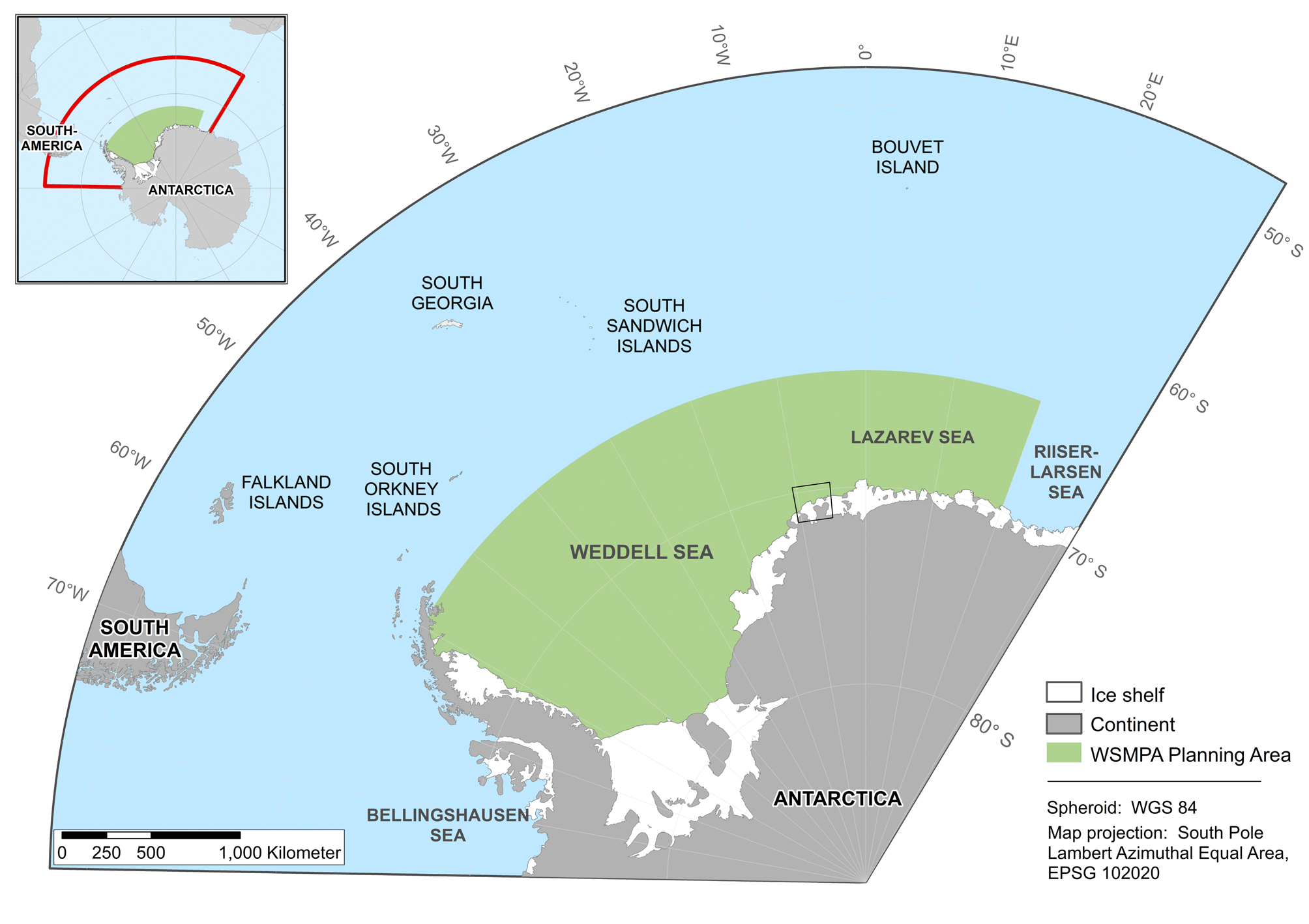
Fig. 1. Study sites at the regional scale (green area) and local scale (black box) in the Southern Ocean (Antarctica). Overview map of the study sites and their locations in the Southern Ocean (top left corner). WSMPA = Weddell Sea marine protected area.
For the model application at a local scale, we studied an embayment off the Ekström Ice Shelf in the eastern Weddell Sea at 70°35'S and 7°51′W, near Atka Bay and close to the German research station Neumayer Station III (Fig. 1). The Atka Bay region includes important areas in terms of biodiversity (e.g. see Gutt et al. Reference Gutt, Griffiths and Jones2013) and is characterized by highly variable ice conditions (e.g. the seasonal character of the fast-ice regime; Arndt et al. Reference Arndt, Hoppmann, Schmithüsen, Fraser and Nicolaus2020).
Data
We used daily high-resolution sea-ice maps of the Southern Ocean provided by the Physical Analysis of Remote Sensing Images (PHAROS) group at the Institute of Environmental Physics (IUP), University of Bremen, Germany. The daily sea-ice raster maps are derived from satellite observations of sea-ice concentration (SIC) produced by the Advanced Microwave Scanning Radiometer - Earth Observing System (AMSR-EOS) instrument on board the satellite ‘Aqua’ or from AMSR2 (the successor of AMSR-E) on board the satellite ‘Shizuku’ (GCOM-W1).
Daily data of SIC from AMSR-E (June 2002 to October 2011) and AMSR2 (since August 2012) were downloaded from the IUP data portal (https://seaice.uni-bremen.de/data/). For our analyses, we used data from 1 January 2002 to 30 June 2020. The ARTIST Sea Ice (ASI) concentration algorithm was used with a spatial resolution of 6.25 km × 6.25 km (Spreen et al. Reference Spreen, Kaleschke and Heygster2008). The downloaded raster data were projected in ‘NSIDC Sea Ice Polar Stereographic South’ (EPSG 3412).
Data processing and analysis
The daily sea-ice raster maps were downloaded as GeoTiff files with the R package RCurl (Lang Reference Lang2021) and then imported into R (R Core Team 2017) with the R package raster (Hijmans Reference Hijmans2021).
Raster data ranged from a minimum grid cell value of 0 to a maximum value of 255. Values between 0 and 200 represent the SIC (0% ≤ SIC ≤ 100%) in 0.5% steps, while values ≥ 201 refer to landmass or missing data. Values ≥ 201 referring to landmass were excluded from the dataset.
The first step in calculating RA is to define the accessibility (A) of a cell at a given time. Accessibility A of grid cell i in year j on day x was given by
 $$A_{i, j, x}\in { {0, \;1} } $$
where A takes the value of 0 (inaccessible) at SIC > 60% and the value of 1 (accessible) at SIC ≤ 60% according to Parker et al. (Reference Parker, Hoyle, Fenaughty and Kohout2014).
Missing SIC data for a specific cell on a specific day of a specific year (see Table S1) were derived from the average accessibility score A for that cell on that day of that year across all years. For those cells with an average accessibility score A ≤ 0.5 (given if at least half of all available years are inaccessible) we have assigned a value of 0 to the grid cell. In case of an average accessibility score A > 0.5 (given if more than half of all available years are accessible) we assigned a value of 1. As the analysis presented here requires the data for 1 day in several directly consecutive years, an analysis of the leap day is not possible. February 29 (which is only present in the datasets of 2004, 2008, 2016 and 2020) was thus excluded from this study. Our SIC dataset covers a total of 6256 days (see Table S1).
We chose to apply our RA calculations to a mark-recapture research fishing scenario as a way to exemplify how they might be used in practice. This scenario had been suggested by the CCAMLR Working Group on Statistics, Assessments and Modelling (WG-SAM) (CCAMLR 2016). In the scenario, the initial study (tagging of fishes) takes place in cell i in year j on day x. The CCAMLR WG-SAM noted that the recapture of tagged fish should be targeted within the next 2 years following year j (i.e. the same cell i should be accessible again in year j + 1 or j + 2). The probability of RA to cell i initially visited in year j on day x is given by
 $$RA_{i, j, x} = \displaystyle{{A_{i, j, x}( {A_{i, j + 1, x} + A_{i, j + 2, x}} ) } \over 2}$$
RAi,j,x is always zero if Ai,j,x = 0 and will only be non-zero if Ai,j,x = 1 and Ai,j+1,x and/or Ai,j+2,x = 1. In the case of accessibility occurring only once within the next 2 years after year j (see requirements above), RAi,j,x = 0.5 and is ultimately set to 1.
For the whole observation series of ny years (here, 19 years in total) the mean RA mRA of grid cell i visited on day x in the respective first year amounts to
 $$mRA_{i, x} = \mathop \sum \limits_{\,j = 1}^{\,j = ny-2} \displaystyle{{RA_{i, j, x}} \over {ny-2}}$$
A summarized overview of all variables used for calculating A or RA and their specification for our case study is shown in Table I. To demonstrate our RA analysis and illustrate the spatiotemporal patterns of RA, we calculated daily and monthly RA scores at a regional scale (i.e. WSMPA planning area) and at a local scale (i.e. Atka Bay).
Table I. Overview of the variables used for calculating accessibility or repeated accessibility.

WSMPA = Weddell Sea marine protected area.
The following R scripts for calculating the RA are available under Zenodo (https://doi.org/10.5281/zenodo.4714531):
1) 'Download of daily sea-ice raster' - the R script automatically downloads all GeoTiffs from IUP, University of Bremen, and saves them in the directory of your choice.
2) 'Existing and missing data' - the R script uses the downloaded GeoTiffs to create a table showing for which days satellite images are available and for which days they are not.
3) 'Information of GeoTiffs' - the R script extracts important metadata of the downloaded GeoTiffs such as geographical projection, spatial extent and maximum value. A metadata table is created.
4) 'Repeated accessibility' - the R script performs the RA calculation based on a selectable threshold of SIC.
Results
Repeated accessibility patterns on a regional scale
The probability of RA for the entire WSMPA planning area is very low in most months (< 20% from early May to mid-December) (Fig. 2). From mid-December, the probability of RA increases continuously to a maximum of 58.02% (± 40% SD) in mid-February. Then, the probability of RA for the area drops again to < 20% at the end of April, but the SD remains relatively high at ± ~30%. RA with a higher probability of ≥ 50% occurs only from mid-January to mid-March.

Fig. 2. Mean repeated accessibility (RA; in %) for the entire Weddell Sea marine protected area (WSMPA) planning area per day (mean values over the years 2002–2020; i.e. the probability that the WSMPA planning area is navigable by vessels at a given time and again within the following 2 years).
The RA spatial pattern for the WSMPA planning area shows an extension of highly repeatedly accessible areas east and west of the prime meridian and from 64°S to almost 70°S from December (RA probability of > 70% ± < 40% SD) through January to February (RA probability of > 90% ± < 10%) (Fig. 3). In addition, smaller areas with the highest RA probabilities extend directly along the ice shelves of the east-south-eastern Weddell Sea as well as the Antarctic Peninsula during this period. From March onwards, the extent of the areas with the highest RA probability decreases again, so that in May there are only areas east of the prime meridian at the northern fringe of our study site that show an 80–90% RA probability (± < 30% SD). From June to November, almost the entire study site is not repeatedly accessible (RA probability of < 10% ± < 10% SD); only a few small areas show a RA probability of > 10%, although mostly only slightly higher (see Fig. S1). A considerable part of the areas west of 30°W show the lowest probability (< 10% ± < 10% SD) of RA throughout the year (Figs 3 & S1).
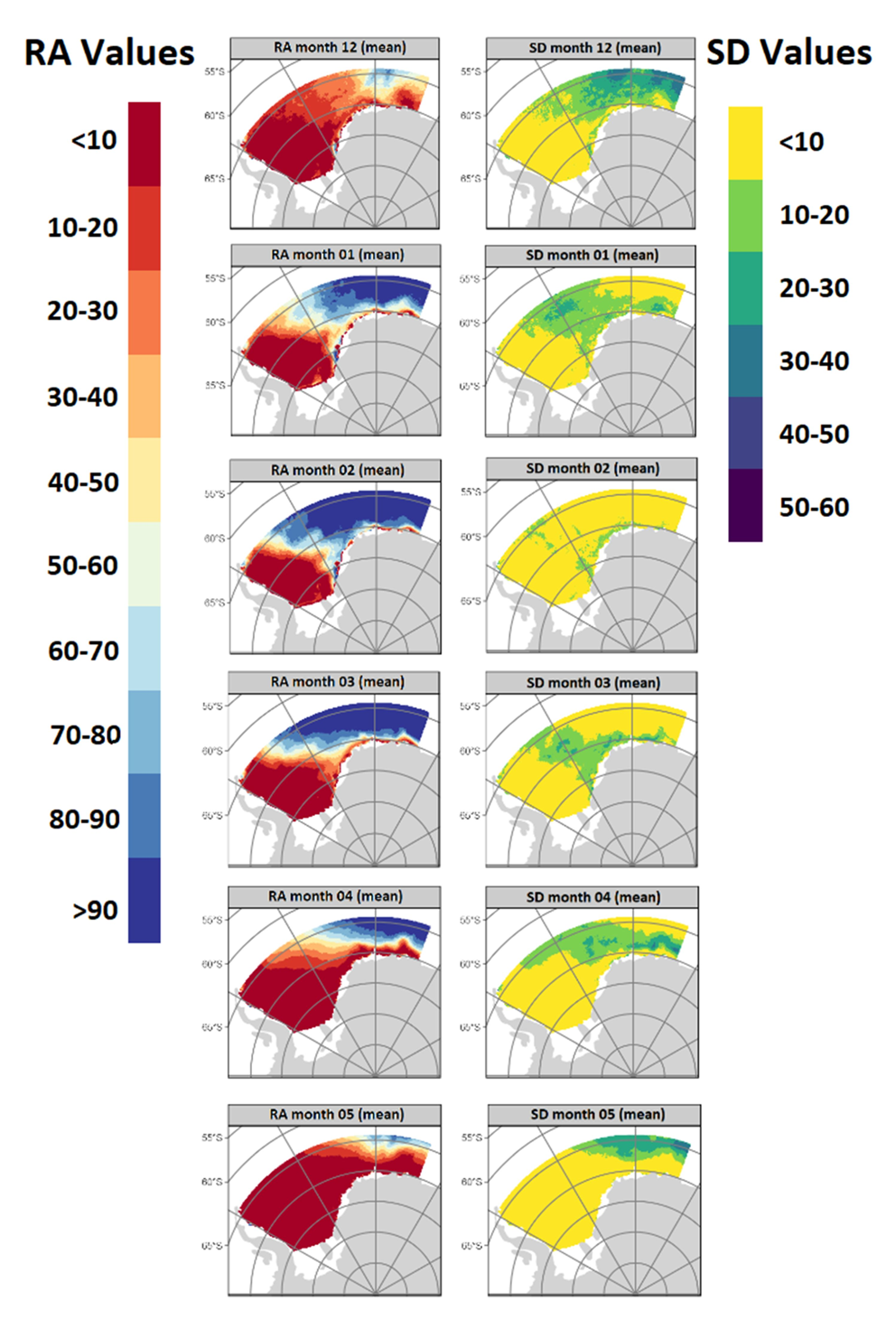
Fig. 3. Mean repeated accessibility (RA; left) ± standard deviation (SD; right) (in %) in the Weddell Sea marine protected area planning area within a 3 year period shown per summer and autumn month (mean values over the years 2002–2020).
Repeated accessibility patterns on a local scale
The RA probability in Atka Bay is similar to that for the entire WSMPA planning area in terms of its intra-annual pattern. The RA of Atka Bay from mid-April to mid-November is very improbable (i.e. < 10% probability that Atka Bay can be navigated by vessels at a given time and again within the following 2 years) (Fig. 4). From mid-November, the RA probability increases continuously until the end of February (22 February: maximum probability of RA = 69.18% ± 15% SD), after which the RA probability decreases again steeply. Only for ~1.5 months (from late January to early March) is the RA probability relatively high (between 60% and 70%).
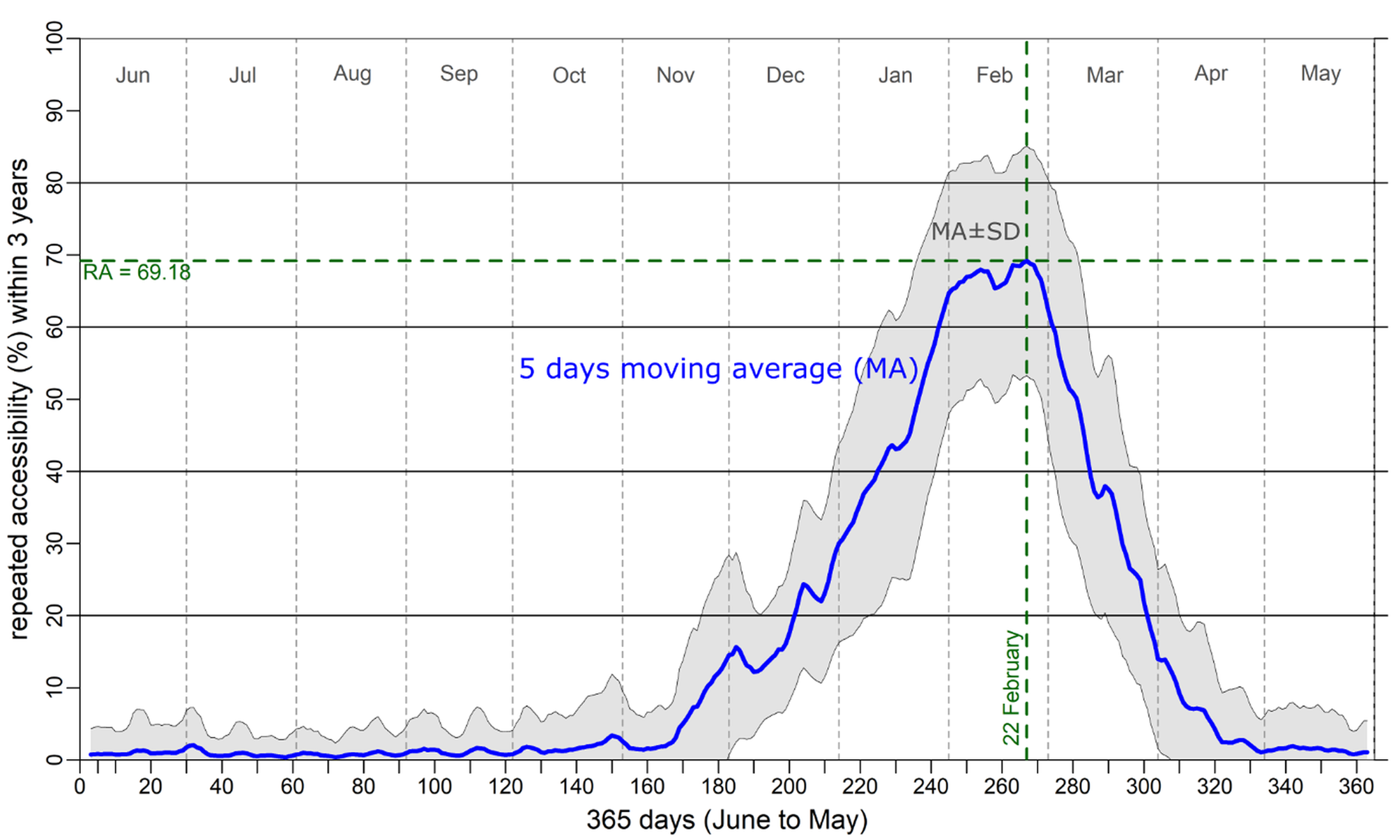
Fig. 4. Mean repeated accessibility (RA; in %) for Atka Bay per day (mean values over the years 2002–2020; i.e. the probability that Atka Bay is navigable by vessels at a given time and again within the following 2 years).
The RA spatial pattern in Atka Bay shows that the area has a RA probability > 60% (± < 20% SD) in February (Fig. 5). In both January and March, only relatively small areas, north of 70°S and near the ice shelf, are repeatedly accessible with a probability of > 60%. From April to the end of November, almost the entire Atka Bay shows a low RA probability (< 10% ± < 10% SD), except for some areas near the ice shelf (Figs 5 & S2). In November, a narrow band emerges along the ice shelf with RA probability values of 10–20% (± 10–20% SD), and in December a spatially mixed picture develops with mostly 10–30% RA probabilities (± < 10–20% SD) (Fig. S2).
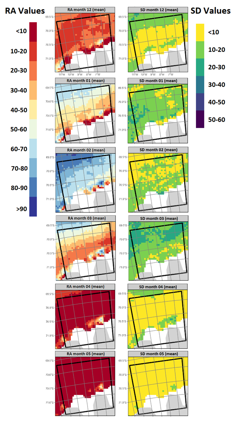
Fig. 5. Mean repeated accessibility (RA; left) ± standard deviation (SD; right) (in %) in Atka Bay within a 3 year period shown per summer and autumn month (mean values over the years 2002–2020).
Discussion
Spatiotemporal patterns of repeated accessibility
The intra-annual pattern of RA probabilities at both regional and local scales reflects the seasonal cycle of sea-ice cover in the Southern Ocean, which is one of the most pronounced signals of variability in the Earth's climate system. The highest RA probability was calculated for February on both spatial scales, while the lowest RA probability occurs from July to October. The calculated RA results match with the seasonal sea-ice dynamics of the Weddell Sea that is covered by thick, partly immobile ice in winter (annual maximum in September) and exhibits ice-free conditions in large areas during the short summer (annual minimum in late February or early March) (www.meereisportal.de).
Spatial distribution of RA probability at the regional scale shows, for example, the lowest RA values (throughout the year) in the central, south-west Weddell Sea, which is known as one of the few regions in the Southern Ocean where multi-year sea ice has been observed (Lange & Eicken Reference Lange and Eicken1991). The spatial distribution pattern of high RA probabilities on the regional scale also matches well with the occurrence of coastal polynyas in the Weddell Sea. Areas characterized by coastal polynyas have been reported, for example, at the tip of the Antarctic Peninsula (e.g. Arrigo & van Dijken Reference Arrigo and van Dijken2003), the central Weddell Sea off the Ronne Ice Shelf (Tamura et al. Reference Tamura, Ohshima and Nihashi2008, Haid & Timmermann Reference Haid and Timmermann2013) or along the ice shelves west of the prime meridian (e.g. Nihashi & Ohshima Reference Nihashi and Ohshima2015).
Similarly, the spatial distribution patterns of low and high RA probabilities along the coastline at the local scale are supported, for instance, by Nihashi & Ohshima's (Reference Nihashi and Ohshima2015) description of ice conditions in terms of fast ice and polynyas at Atka Bay.
Limitations and strengths of the tool
The RA tool considered the SIC for each grid cell, for each day in each year, and assigned values of 0 (inaccessible) or 1 (accessible) to each SIC value, depending on whether the predefined SIC threshold was exceeded or not. Given a set start year, it then computed whether RA occurred (i.e. at least one more accessibility event was recorded) during a predefined timespan. If RA had occurred for the specific start year and its subsequent years, a value of 1 was assigned to this individual run; otherwise the run was assigned a score of 0. This check was applied to all possible start years and respective subsequent years (within the predefined timespan) for each day. Then, the score sum of the individual runs (with different start years) per day was divided by the maximum possible number of individual runs and multiplied by 100. Thus, the mean RA probability of a grid cell for the respective day was expressed by taking into account the different years within the set timeframe.
Accordingly, our tool cannot provide information on temporal patterns such as recurring intervals (e.g. years with low ice concentration alternating with years with high ice concentration) or trends in SIC across years. Furthermore, the RA value of a specific raster cell does not indicate whether this raster cell can actually be reached by ship. For example, many coastal areas have a relatively high RA value (i.e. high RA), but cannot be reached by non-ice-strengthened ships because these areas are completely surrounded by dense sea ice. Other ice properties that are important for navigation, such as the age of the ice, ice thickness and ice drift, are also not taken into account by our RA tool. Nevertheless, our tool is a useful first step to get a quick overview of an area's possible RA during a certain period of time. This is especially important with regards to scientific sampling, as often sampling designs require repeated sampling within a set timeframe. The threshold value for the calculation of RA can be amended as desired (e.g. 80% SIC instead of the 60% SIC used here); this allows RA values to be customized to more accurately reflect prerequisites of different ships and their ice classes.
In conclusion, the results of our spatiotemporal RA analyses are successful in reflecting known characteristics of sea-ice distribution and dynamics in the Weddell Sea, confirming the functionality of our simple tool for determining RA of a certain area. As a next step, we aim to develop algorithms that also incorporate the ‘in/out path’ from A to B for a larger area based on the empirical SIC data, taking into account vessel characteristics (ice class, speed) and trade-offs (distance vs probability). The module is ultimately intended to provide a service for relevant stakeholders and scientific knowledge gain (e.g. to answer the question of how the probability spaces change when ice conditions change due to climate change).
Acknowledgements
We thank two anonymous reviewers for constructive comments on the manuscript.
Financial support
This work was financially supported by the German Federal Ministry of Food and Agriculture (BMEL) through the Federal Office for Agriculture and Food (BLE), grant numbers 2813HS009 and 2819HS015. We acknowledge support by the Open Access Publication Funds of Alfred-Wegener-Institut Helmholtz-Zentrum für Polar- und Meeresforschung.
Author contributions
HP and TB jointly developed the approach, HP performed the data analysis and KT initiated and led the writing of the paper with contributions from HP, RK and TB.
Supplemental material
Two supplemental figures and a supplemental table will be found at https://doi.org/10.1017/S0954102021000523.


 Open access