


Introduction
Traditional methods of glacier inventory have used vertical and oblique aerial photographs as the primary source of information. For more than a decade, however, Landsat multispectral scanner (MSS) imagery has been providing up-to-date, repetitive coverage of the Earth’s surface. Such imagery is, therefore, a potential data source for the preparation of regional glacier inventories.
Examples of the capabilities of Landsat imagery for displaying information about glacial environments were presented in the United States Geological Survey Professional Paper 929, entitled “ERTS—1: a New Window on our Planet” (Reference Williams and CarterWilliams and Carter, 1976). Landsat imagery was also featured in the First Symposium on Remote Sensing in Glaciology held at Cambridge, England in 1974 (Reference Krimmel and MeierKrimmel and Meier, 1975; Reference ØstremØstrem, 1975), In all of the above papers, analysis of Landsat was carried out in its visual format. Reference Rundquist, Collins, Barnes, Bussom, Samson and PeakeRundquist et al. (1980), however, used digital Landsat data to produce plots from supervised classifications, showing selected glacial features, for several ice masses and mountainous areas. A search of the more recent literature suggests that little recent work has been done to assess the capabilities of digital Landsat data for studying glacial environments. The aim of this paper is to identify the role that Landsat digital data can play in providing information to be used in preparing glacier inventories. Studies have been carried out, using glacier inventory data and Landsat MSS imagery, for two parts of Canada: the Steacie Ice Cap on Axel Heiberg Island and the Kaskawulsh Glacier in the St. Elias Mountains.
Steacie Ice Cap
Located at 79°N, 90 °W, the Steacie Ice Cap occupies the south-western corner of Axel Heiberg Island. Being representative of the ice caps of the high Arctic and physically separated from the other ice caps of Axel Heiberg Island, it provided a good site for a pilot study for a glacier inventory in the high Arctic (Reference OmmanneyOmmanney, 1969; Reference Ommanney1970). It was, therefore, an equally suitable location to test the capabilities of Landsat imagery for providing area measurements in glacier inventory studies.
Methodology
Analysis was carried out at the Canada Centre for Remote Sensing, using their image analysis system (CIAS). A subscene, measuring approximately 90 km by 90 km, which included the entire Steacie Ice Cap was selected from image 20948-18430, recorded on 27 August 1977 (Path 60, Row 2). The late August image was selected as being representative of ground conditions at the end of the ablation season. The solar elevation angle was fairly low when the satellite recorded the imagery early in the morning. Although this helps to show detail in the topography, due to shadow, radiance from the terrain is not high. As a result, the initial image recorded on the colour monitor of the CIAS was dark. A linear, contrast stretch enhancement of the digital data gave detail in the terrain and also emphasized the margins of the ice cap and outlet glaciers.
A supervised classification was carried out to identify all areas of snow and ice. Manipulation of the spectral range in each of the four MSS bands was undertaken, to ensure that all areas were included in the classification.
A Versatec electrostatic printer was used to produce a 1:125 000-scale map, the same scale as the original compilation of the glacier inventory. One map of the area was produced as a 16-level grey-tone print from the linear contrast stretch enhancement of the Landsat MSS band 5 image (Fig.1). The other was a thematic map of the supervised classification of the Landsat digital data. The maps prepared from the Landsat imagery were compared with the maps of the Steacie Ice Cap produced and described by Ommanney (Reference Ommanney1969; Reference Ommanney1970).
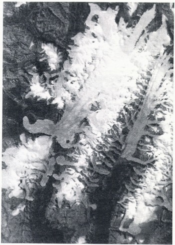
Fig. 1 A grey-tone print of part of the Steacie Ice Cap. The Good Friday Bay Glacier, a tidal, outlet glacier, can be seen, left, where it terminates in a fjord. The width of the area shown is approximately 60 km.
Results
The supervised classification, which was expected to provide an accurate measure of the areas of snow and ice, was a difficult task for several reasons. First, there is spectral similarity between the darker areas of the ice and some of the rock surfaces illuminated by the sun in the surrounding terrain. As a result, parts of these rocks became classified as snow or ice. The only way to overcome this problem was to identify and remove the anomalous pixels from the displayed image by means of the cursor on the colour monitor; a time-consuming and laborious task.
A second problem occurred around the nunataks on the ice cap. Rock surfaces, illuminated by the sun, became classified as snow and ice, while areas of snow and ice in shadow were too dark to be included in the classification. To a certain extent, these errors in pixel identification tend to cancel each other out when the total area of snow and ice is calculated, but it is certainly not an ideal situation for making accurate measurements.
A final problem is that there are several, large, glacial lakes which, during most years, maintain an ice cover, even at the end of the ablation season, Although an experienced photo-interpreter may be able to identify the locations and extent of these lakes from stereoscopic aerial photographs, this is not possible with the satellite imagery. To the MSS on Landsat, snow-covered lake ice has exactly the same properties as snow-covered glacier ice; therefore, the two cannot be differentiated.
Although area estimates can only be made very approximately, the 16-level grey-tone print proved very useful. It was possible to overlay the original glacier inventory on the print and check for any discrepancies on a light table. On the Steacie Ice Cap, it was noted that the Good Friday Bay Glacier was the only glacier to have changed appreciably since 1959, the year in which the aerial photography used for the glacier inventory was acquired. The glacier has advanced approximately 5 km since 1959 (Reference Howarth, Ommanney and WellarHowarth and Ommanney, 1983). It now ends in the fjord and is the only iceberg-producing outlet glacier of the Steacie Ice Cap.
Kaskawulsh Glacier
The Kaskawulsh Glacier is an active valley glacier in the St. Elias Mountains. Studies were concentrated on both the lower part of the glacier and its pro-glacial area, although the firn zone was also analysed. When image 21314-19293 was recorded on 28 August 1978 (Path 66, Row 17), ground conditions were typical for the end of the ablation season. Bare ice, displayed in light blue on the colour monitor, contrasted well with the dark grey of the medial moraines. Ice and permanent snow patches in the surrounding mountains stood out against the darker background of the rock surfaces. At lower elevations, vegetation was displayed in red.
Methodology
Using a supervised classification, it was possible to map several of the categories identified in the glacier inventory map; glacier ice, debris-covered ice, pro-glacial lake. Attempts were also made to separate snow, ice, and the firn zone. After a linear contrast stretch of all four MSS bands of the original dark image, a 16-level grey-tone print of the MSS band 5 image at a scale of 1:50 000 was produced on the Versatec plotter (Fig.2).
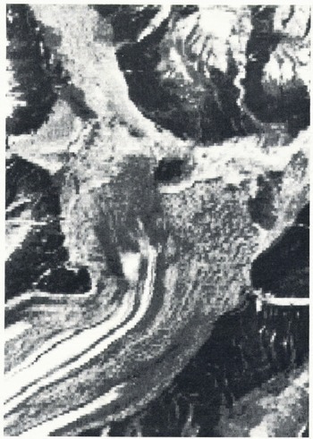
Fig. 2 A grey-tone print of part of the lower section of the Kaskawulsh Glacier and its pro-glacial area. Note the ice margin, identified by the abrupt change in tone and the textured pattern of dark and light pixels, indicating a hummocky surface on the right side of the glacier. Original scale of the print was 1:50 000. The width of the area shown is 11 km.
Results
With the supervised classification, it was possible to separate snow and ice. A transition zone, perhaps wet firn, occurred on all major tributary glaciers, but it was also encountered around many of the nunataks, where it probably represents areas of shadow or boundary pixels between snow and rock.
In the lower part of the glacier, the glacier ice and pro-glacial lake were spectrally distinct and readily classified. Debris-covered ice, however, showed spectral confusion with valley side slopes and the pro-glacial area. With similar rock types in all (hese environments, the result is not surprising.
In this image, vegetation was not included in the classification, nor were the unvegetated mountain slopes. The potential complications of the highlights and shadows in any classification of the valley side slopes can readily be appreciated.
Through interpretation of the enhanced image, however, it was posssible to identify much detail in the marginal zone of the glacier. The darker grey colour of the moraine on the glacier could be differentiated from the lighter tones of the pro-glacial area. A pattern of lighter and darker pixels indicated a hummocky surface on part of the glacier terminus and shadows identified where the ice front was steep. Subtle vegetation outlined an end moraine, and braided channels of a valley train gave a light blue colouration to the image.
The grey-tone print was important. It showed many of the features seen in the enhancement and could also be used as a base on which to record information observed from the enhanced Landsat image.
Conclusions
On the basis of these two preliminary studies, it is possible to draw the following conclusions:
-
1. As a substitute for aerial photography, to provide detail required for glacier inventory, Landsat MSS digital data, with its approximately 60 m by 80 m pixel resolution, is not the answer.
-
2. Measurement of the surface area of snow and ice can only be done approximately. This is because of errors introduced by spectral confusion of snow and ice with rock outcrops, illuminated by the sun. In addition, shadows cause snow and ice to be incorrectly identified and the problem of differentiating ice covered lake from glacier ice also leads to errors.
-
3 For interpretation and mapping in the pro-glacial area, enhanced Landsat images are preferable to classification.
-
4. The major advantage of Landsat MSS imagery is the ability to prepare rapidly a base map, on an electrostatic printer, at the scale of the existing, glacier-inventory maps, Landsat may then be used to identify visually areas of major changes, as a basis for updating the existing inventory.
Acknowledgements
Financial support for this study was received from the National Hydrology Research Institute of Environment Canada and the Natural Sciences and Engineering Research Council of Canada (Grant No. A0776).


