


Introduction
The snow cover in pre-Alpine regions is often very heterogeneous due to both the topography and the forest canopy which at that altitude (1000–1500 m) is quite extensive. It is also the zone where in normal winters the snow cover is subjected to intermediate thawing and refreezing. Improved knowledge of the spatial variation of the snow cover in that zone is important because
-
(i) meteorological models, having a typical resolution of a few km2, are still poor at simulating heat exchange over a patchy snow cover, and this can be rectified only by decreasing the resolution and including sub-grid variability;
-
(ii) to improve the prediction of snowmelt runoff in hydrological catchments we need to account for the considerable variability of the snow water equivalent (SWE) as input to the forecast model.
Here we shall show an approach to characterize and quantify the variation of the snow cover within a 0.7 km2 catchment using linear regression analysis. In addition to characterizing the variation of the snow cover, the aim was to come up with a simple tool to predict the temporal and spatial development of the snow cover within the catchment.
Measurements
Spatial measurements of the snow depth were carried out on 5 days of winter 1998/99, and on 2 days of winter 1999/2000 in the 0.7 km2 catchment Erlenbach, central Switzerland (Fig. 1). The catchment consists of a mixture of open pasture and marshy meadow, and of closed and sparse forest (about 40% forest). The sampling locations were distributed on a regular grid (spacing 75 m) which covered the whole area from the crest at 1600 m to the stream outflow at 1100 m. In both the upper and the lower parts of the catchment, another 40 sampling points were added on a 25 m grid in order to catch the variation at a minor resolution. At each location, snow depth was measured at five points within a circular area of 4 m2 to level out the very small-scale heterogeneity of the soil surface. Slope, aspect and altitude were determined, and each location was classified as (a) open land, (b) semi-forested or forest edge, (c) closed forest or (d) wind-exposed (close to the ridge). For the forested locations (classes (b) and (c)) the canopy density was determined using a simple quantitative method (Reference Stahli, Papritz, Waldner and ForsterStahli and others, 2000): at each point we photographed the canopy from below and digitized the picture. Using a simple threshold operation in the blue channel, we classified the pixels forming the canopy and used their relative frequency as a measure for the canopy density, dc.

Fig. 1. Map of the Erlenbach catchment. The shadowed areas represent the forest cover. (Reproduced by permission of Bundesami für Landeslopographie, BA4813.)
Data Analysis
To explore the influence of topography and vegetation on the spatial snow-cover pattern, linear regression models were fitted for each measurement date. Two regression models were tested, one model (A) where the site-specific topography and vegetation were accounted for using continuous variables, and one simpler model (B) where the locations were represented only in terms of indicators and the altitude:
Model A:

Model B:
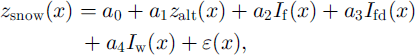
where zsnow is snow depth (cm), zalt is altitude (m), dc is canopy density (-), st is slope (m m–1), et is aspect in terms of deviation from south and ε(x) is an error term. Iu Iid and Iwe are indicators for forested locations, closed forest and wind-exposed locations according to the following scheme:
We investigated whether the error term of the regression model showed spatial dependence by computing the experimental variograms of the residuals, rsnow(x), using the formula
where γ(h) is the semivariance, h is the lag distance between two data points and n is the number of data points.
Finally, a time-space linear regression model describing both the temporal development and the spatial distribution of the snow cover was evaluated. To explain the temporal development we included the sum of positive daily air temperatures, Taacc, and the accumulated snow precipitation, Psacc starting from the first day of observed snowfall (Fig. 2) in the model. These meteorological variables were taken as measured at the Erlenhohe meteorological station (see Fig. 1). The spatial patterns were modeled by the same explanatory variables as in models A and B above, but we included in addition their interactions with Taacc and Paacc to allow for temporal changes in the spatial patterns. Influential effects and interactions were determined by a stepwise forward procedure. This resulted in the following models:
Model A (only open-land locations):
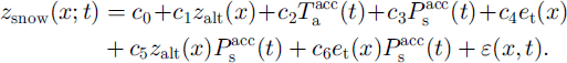
Model A (only forested locations):

Model B:


Fig. 2. Sum of positive daily air temperatures (°C) and accumulated snow precipitation (mm) for the two winters 1998/99 and 1999/2000, measured at the meteorological station Erlenhohe (1230 m a.s.l.).
The coefficients ci were determined from the five snow-measurement dates of winter 1998/99. Finally, these time-space linear regression models were validated with the data from the snow measurements of winter 1999/2000.
Results
Winter 1998/99 was exceptional with respect to snow accumulation. After a rather early first snowfall in mid-November and a moderate snowpack of about 0.5 m at the end of January, heavy snowfall produced a snow depth of up to 150 cm in the lower part of the catchment, and up to 300 cm in the upper part (Fig. 3). A maximum SWE of 1012 mm was measured on 1 March in a shallow depression close to the crest. The main snowmelt started on 20 April and lasted about 1 month until all the snow in the catchment had disappeared.

Fig. 3. Area-averaged snow depth (cm) calculated with the two tine-space linear regression models (lines) and measured (symbols).
Winter 1999/2000 took a similar course. On the day of our first measurement (23 December) the average snow depth in the catchment was 0.7 m, corresponding to a SWE of 204 mm, which was somewhat more than in December and January of the previous winter. Later on, the snow cover again developed very similarly to that in winter 1998/99. After the maximum accumulation in early April with an area-averaged snow depth of 150 cm, the snow melted rapidly to the end of May.
The considerable spatial variation of the snow cover showed two main trends, which became more distinct the longer the winter lasted: first, the snow depth increased with increasing altitude, and, second, it decreased with increasing canopy density. On average, the snow depth in the forested areas was about half of that found in open-land areas (Reference Stahli, Papritz, Waldner and ForsterStahli and others, 2000), which is in agreement with long-term snow course measurements in the neighborhood (Keller and others, unpublished).
The linear regression analysis (Equations (1) and (2); Table 1) for the individual measurement dates showed that:
Model Awas able to explain 41–77% of the snow-depth variation in the whole catchment.
The simpler indicator model (model B) had some lower coefficients of determination (R2 = 0.36–0.57) than model A and significantly smaller standard deviations.
The lowest coefficient of determination was reached for the measurement date during the final snowmelt period (10 May 1999) when the snow cover was patchy. This applies particularly to the forested locations for which the R2 value was 0.13 using model A. This implies that dc was not a suitable measure to describe the effect of the forest canopy on the snowmelt.
On the other hand, for the snow-accumulation period (December-March) there was no substantial difference between the goodness of fit of model A in the open-land area and in the forest. This is surprising since the snow-accumulation pattern was expected to be more complex below the canopy.
Table 1. Coefficient of determination and residual standard deviations (cm) for the two linear regression models of zsnow(x) applied to single days of the two winters

We computed the experimental semivariograms of the residuals of the linear regression model B for two measurement dates (Fig. 4). The lack of a distinct dependence of the semi-variances on the lag distance on 15 December signals that the spatial autocorrelation of the error term was at most very weak for that measurement date. On 22 January, however, the semi-variance increased to 0.4 km and reached a constant level (sill) beyond that distance. But the autocorrelation was also rather weak because at the shortest lag distance the semivariance equaled roughly half of the sill.

Fig. 4. Experimental semivariograms of the residuals of the regression model B for 15 December 1998 and 22 January 1999
The time-space linear regression models (Equations (5–7)) were able to explain 61–77% of the spatial and seasonal snow-depth variability of winter 1998/99 (Table 2), which can be considered satisfactory in view of the simplicity of the models. Only minor differences between the models were seen with regard to the coefficient of determination and the residual standard deviation. Also the time development of the area-averaged snow depth (Fig. 3) was very similar between the regression models. They fitted satisfactorily with the area-averaged mean of the snow-depth measurements of the first winter. For the validation winter of 1999/2000 the simulated area-averaged snow depth was in close correspondence with that measured on 23 December, but overestimated the mean snow depth on 4 April by approximately 25 cm. Comparing qualitatively the maps of measured and calculated snow depth (Fig. 5), interpolated on a 25 m grid using an inverse quadratic distance gridding method, showed that the general patterns of the snow-depth distribution were well reproduced by the models. For example, the influence of the forest cover (cf Fig. 1) and some areas with a thick snow cover corresponded well. The measured spread of snow depth within the area was better reproduced by model A than by model B (cf. standard deviation, maximum and minimum in Table 3), but for the April measurement it was clearly underestimated by both models. The coefficient of determination R2 was within the range 0.51–0.75 for the two validation measurements (Table 3).

Fig. 5. Map of measured and simulated snow depth (cm) interpolated with an inverse quadratic distance gridding method for 23 December 1999 (left) and 4 April 2000 (right).
Table 2. Coefficient of determination and residual standard deviations (cm) for the time-space linear regression models of zsnow (x, t) fitted to the measurements of winter 1998/99
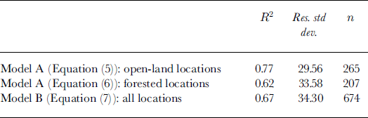
Table 3. Statistics for simulated and measured snow depth for the validation winter 1999/2000

Discussion and Conclusions
Whereas the magnitude and the temporal development of the snowpack may vary considerably from year to year, its pattern, i.e. the spatial distribution within a certain landscape, remains basically the same due to characteristic surface properties (e.g. Reference Konig and SturmKonig and Sturm, 1998). This fact has to be made use of when we want to quantify sub-grid snow-cover variability by applying regression models that contain key parameters forming this pattern. For such models to be useful, the number of parameters must be kept at a minimum and they must be easily determinable at the sub-grid scale from available databases, geographic information system, maps, aerial photographs or similar products. Several works along these lines have already been reported (e.g. Reference Elder, Davis and RosenthalElder and others, 1997; Reference ForsytheForsythe, 1999) pointing out the most influential parameters for different watersheds and stages of the winter.
In this paper we tested such an approach for an area with rather uniform topography but complex vegetation structure at a scale where repeated snow-depth measurements are seldom available. The results were encouraging with regard to the simulation of the spatial snow-cover patterns, e.g. when looking at the goodness of fit for the validation measurements of winter 1999/2000. But also with regard to the temporal simulation of the area-averaged snow depth, the time-space linear regression models, simply based on accumulated snow precipitation and positive daily air temperature, were a satisfactory tool. Of course, there is still a wide range of possible refinements of the models (e.g. a better measure of the canopy density must be found, which will be a main point of investigation in our future work with the Erlenbach catchment). But one has to keep in mind that the model must remain simple in order to become a useful tool.
Although the semivariograms of the residuals and the error term are not the same (cf. Reference CressieCressie, 1993, section 3.4), and proper inference about the spatial autocorrelation of the error term should be better based on a parametric approach (Reference KitanidisKitanidis, 1983), we believe that one should not assume that the error terms ε(x, t) were spatially and temporally independent. This has two consequences. First, significance testing based on the F-test is invalid in the regression analysis. Therefore, we used the coefficient of determination as a purely descriptive measure for the quality of the model fit. Second, it might be advantageous to use a geostatistical approach for spatial mapping of the snow depth. Universal kriging (Reference CressieCressie, 1993, section 3.4) is a candidate method because it combines a linear regression model for the systematic trends in the variation with mean square prediction of the stochastic error term. In the future, we will investigate this further. The problem of sub-grid variability of larger-resolution deterministic models, such as mesoscale snow models or global circulation models, is an issue of high interest in current snow research (Reference BlöschlBlöschl, 1999). Where the spatial arrangement of, for example, the SWE is less important than its fraction per grid unit, it might be useful to work with snow-depletion curves (Reference Luce, Tarboton and CooleyLuce and others, 1999). However, where sub-grid variability must include information about the pattern, a promising approach might be to distribute the snow cover according to a few simply determinable land-surface parameters with regression models.


