1. INTRODUCTION

In the past few years, experiments have been successful in measuring the CO₂ concentration of air trapped in bubbles in old polar ice. In this way, it has been possible to reconstruct the anthropogenic CO₂ increase, and it has been found that atmospheric CO₂ levels were lower in glacial than in postglacial time. There are also indications of natural CO₂ variations during the past millennium (Reference Raynaud and BarnolaRaynaud and Barnola 1985), and we present data here that point to a CO₂ input into the atmosphere during the thirteenth century. For a better understanding of the observed variations, it is of interest to know the carbon-isotopic composition of the trapped C0₂. Since biomass and fossil fuels have relatively low δ¹³C values, of about –25‰ (compared with δ¹³C % –7‰, for atmospheric CO₂), a CO₂increase due to input of biospheric or fossil fuel CO₂ is accompanied by a decrease in δ¹³C. On the other hand, a CO₂ change due to a net transfer between ocean and atmosphere is expected to have little influence on δ¹³C.

We have developed a method for extracting the CO₂ from air trapped in ice and for measuring its carbon- and oxygen-isotope ratios by mass spectrometry (see section 2). We applied this method in order to determine the δ¹³C trend accompanying the CO₂ increase over the past 200 years (Reference Friedli, Lótscher, Oeschger, Siegenthaìer and StaufferFriedli and others 1986). In this paper (section 3) we reconsider a series of CO₂ and δ¹³C results obtained from samples spanning the period of about 1000–1800 A.D., taken from an ice core from the South Pole (Reference Friedli, Moor, Oeschger, Siegenthaìer and StaufferFriedli and others 1984).

In addition to δ¹³C, δ¹⁸O was routinely determined in our measurements. Atmospheric CO₂ has a δ¹⁸O value (versus PDB standard) near 0‰. However, we found values in CO₂ extracted from ice of c. –20 to –30‰o, which shows that the oxygen-isotope composition must have changed between the time the air was trapped in the firn and the time it was measured in the laboratory. We suggest that CO₂ equilibrated isotopically with the ice – in other words, that an exchange of oxygen atoms took place. This is discussed in section 4.

2. EXPERIMENTAL METHODS

The procedures for extracting the enclosed air from the ice and for separating CO₂ from air have been described previously (Reference Moor and StaufferMoor and Stauffer 1984, Reference Friedli, Moor, Oeschger, Siegenthaìer and StaufferFriedli and others 1984). Briefly, the first step involves crushing the ice sample (typically about 700 g) in an evacuated, all-metal extraction system at –20 °C and collecting the air by condensation at a temperature of 15 K. After measurement by gas chromatography of the CO₂ concentration, CO₂ is separated at liquid-nitrogen temperature; volumetric determination of the quantity of CO₂ makes it possible to check the separation efficiency, or, where no result from gas chromatography is available, to measure the CO₂concentration. The CO₂ sample (typically 15 μl) STP) is then transferred to the mass spectrometer (MAT 250), which is equipped with a small-volume inlet system. Achieved overall precision (1 standard deviation) for δ¹³C is O.10‰ in good conditions. For δ¹⁸O the standard deviation is larger, nearly 1‰o. The reason must be oxygen-isotope exchange of the CO₂ with water films adsorbed at the walls of sample-containers and extraction systems. (The precision of the ¹⁸O analysis by mass spectrometry alone is O.1–0.2‰ for samples of about 15 μl STP.)

The results of mass spectrometry have to be corrected to take into account the influence of N₂O, which is separated from air simultaneously with CO₂ in our freezing-out method. N₂O has the same main isotopie masses (44, 45 and 46) as CO₂ and, if the N₂O/CO₂ mixing ratio is known, the correction can be determined (Reference Mook and HoekMook and van der Hoek 1983). We have determined the corrections for our mass spectrometer, and we have developed a method for approximate determination by mass spectrometry of the N₂O/CO₂ ratio, by measuring the abundance of mass 30 which corresponds to the molecule fragment NO⁺ (Reference Friedli and SiegenthaìerFriedli and Siegenthaler, in press). In the course of our work we found that N₂O was produced in a Penning cold-cathode manometer (it must have been formed from N₂ and O₂ in the electric discharge). For the early isotope results (samples from South Pole) we cannot give a precise correction for this effect, so they are less accurate than our later data (samples from Siple Station).

For testing the whole experimental procedure, we routinely processed artificial standard air, and during some measuring periods we noticed systematic deviations in the isotope results of the order of 0.1–0.2‰, the cause of which we could not identify. The question thus arises whether δ¹³C results for samples should be corrected accordingly or not. Such deviations found in "standard-air" samples affect the data for the South Pole series, as discussed in the next section. For the Siple Station series (δ¹³C trend over the past 200 years) (Reference Friedli, Lótscher, Oeschger, Siegenthaìer and StaufferFriedli and others 1986), the standard-air measurements fortunately did not exhibit systematic deviations, only the usual scatter around the mean.

3. CO₂ and δ¹³C RESULTS FROM A SOUTH POLE ICE CORE

Figure 1 shows CO₂ results, obtained by gas chromatography and by volume, and δ¹³C results for samples from a core drilled in 1982 at the South Pole; the ¹³C data have already been published by Reference Friedli, Moor, Oeschger, Siegenthaìer and StaufferFriedli and others (1984). Between A.D.1210 and 1310 the CO₂ concentration increases from 280 to 286 ppm and slowly decreases afterwards. The gas ages given here are based on the assumption that the air in the firn is well mixed. Because of uncertainties about this assumption and about the ice dating, we estimate the error in the gas ages to be about half a century. With reference to the analytical precision, this increase is significant, and it is shown independently by the gas-chromatography and the volumetric concentration measurements. The δ^l3C data in Figure 1b were corrected by +0.25‰ to allow for the presence of N₂O, with an assumed N₂O concentration of 285 ppb (the data given in Reference Friedli, Moor, Oeschger, Siegenthaìer and StaufferFriedli and others (1984) were not corrected). In Figure 1c, average δ¹³C values for the four groups of samples centering on A.D. 1210, 1310, 1430 and 1550 are shown. As mentioned above, the standard-air isotope results were not constant during that period, so standard-air corrected data are also given in Figure 1c. These corrected data vary antiparallel to the CO₂ concentration, reaching a minimum in A.D.1310. It is not possible to decide whether the δ¹³C data are more reliable with or without standard-air correction, so we will consider both possibilities.

Fig. 1. Analytical results versus average gas age for samples from the South Pole ice core, (a) CO₂ concentration, measured by gas chromatography (triangles) and volumetrically (squares). The solid line connects average values for different age intervals, (b) δ¹³C results (standard-air corrected, cf. text); the solid line connects average values, (c) Average δ¹³C results, solid line: standard-air corrected; dashed line: not standard-air corrected.

If the CO₂ results reflect a true atmospheric variation (which can only be determined by measuring more samples from other ice cores covering the same period) then an input of CO₂ into the atmosphere must have occurred in the thirteenth century. In the following we will estimate the size of this input. First, the fact must be taken into account that the air enclosed at a specific depth is not the same age in all the bubbles, because closing of pores at the firn–ice transition occurs over a finite range of densities. Reference Schwander and StaufferSchwander and Stauffer (1984) estimate that at the South Pole the width of the gas-age distribution, defined as the time during which between 10 and 90% of the final volume of bubbles were trapped, is 220 years. Therefore, variations in atmospheric composition which occur over characteristic times less than 220 years will be suppressed in the ice. Reference Neftel, Oeschger, Staffelbach and StaufferNeftel and others (in press) developed a method for back-calculating the atmospheric concentration history from the ice-core record; by frequency filtering they avoid unrealistic high-frequency oscillations in the atmospheric concentration. Figure 2 shows the result of such a back-calculation, using a Gaussian curve for the age-distribution curve of the trapped air. The calculated atmospheric increase is 10 ppm instead of the measured 6 ppm, and there is a slight decrease in concentration before the increase; if the atmospheric CO₂ level had been constant before increasing, then the air with the average trapping-time of A.D.1210 should, because of the broad age distribution, already have had slightly enhanced concentration.

The increase by 10 ppm corresponds to a change in the atmospheric CO₂ mass of about 20GTC (1 GTC = 10⁹metric tons of carbon). In addition, the enhanced atmospheric concentration must have brought about a net CO₂ flux into the ocean. If N_a is the atmospheric CO₂ mass, deduced from the ice-core measurements, the input rate p(t) can be calculated from a CO₂ balance for the atmosphere:

(1)

We calcultated the induced flux into the ocean, F_ao, using the box-diffusion model of Reference Oeschger, Siegenihaler, Schotterer and GugelmannOeschger and others (1975), calibrated by means of bomb-produced ¹⁴C and starting from an assumed steady state at 280 ppm; the procedure has been described in detail by Reference Siegenihaler and OeschgerSiegenthaler and Oeschger (1987). This is how we calculate p(t), which may represent an input from land vegetation or soils or from a restricted part of the world ocean.

Fig. 2. Atmospheric concentration, calculated by deconvolving the ice-core record for the finite time interval of air occlusion.

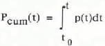
In Figure 3, the input rate p(t), calculated from the model, and the cumulative input

are shown. According to these results, a cumulative input of about 45 GT C over the period A.D. 1200–1350, or about 35GT C net from A.D. 1000 to 1350, would have been necessary to cause the observed concentration change, and the annual emission amounted to up to 0.4 GT C year⁻¹. (For comparison: nowadays about 5 GT C year^1- of CO₂ are produced by fossil-fuel burning.)

Fig. 3. (a) CO₂ input rate (GT C year⁻¹) to produce the atmospheric CO₂ variations (cf. Fig. 2), calculated using the carbon-cycle model. (b) Cumulative CO₂ input (GTC). (c) Solid curve: atmospheric δ¹³C variation calculated from the model, for the assumption that the input was of biospheric origin; squares: observed δ¹³C values (standard-air corrected).

Before discussing the results further, we must emphasize that all the estimates are based on the hypothesis that the CO₂ variation observed in the ice cores indeed reflects an atmospheric change. However, we cannot exclude the possibility that it is an artefact, due to the enclosure process or ice–gas interaction, until further high-precision measurements have been made on a different ice core. This should be kept in mind for what follows.

The presumed input in the thirteenth and early fourteenth centuries could originate from the biosphere or from some region of the ocean. The amount of roughly 40 GT corresponds to about 6% of the global pre-industrial live land biomass, and to about 2% of the total biomass including soils, which are quite appreciable fractions. The period in which the CO₂ input would have occurred coincides roughly with a late-medieval warm phase as registered in England, so one might speculate that the enhanced temperature could have led to higher soil respiration rates and thus to a net transfer to the atmosphere of carbon from soils. It has been well established in experiments that on a short-term (monthly) basis CO₂ production in the soil is correlated with (monthly) temperature (Reference Dörr and MünnichDörr and Münnich 1987), but it is not clear whether the net production also varies significantly with temperature over the time-scale of a century. In theory, human activity like deforestation and agricultural expansion in Europe and the Mediterranean region could also be responsible for the increase in CO₂, but the cumulative input seems rather large for that to be the case.

A biospheric input would cause a decrease in δ¹³C in atmospheric carbon dioxide. Figure 3c shows the isotopie variation calculated with the carbon-cycle model, based on the assumption that the CO₂ input of Figure 3a consisted of biospheric CO₂ with δ¹³C = –25‰. The measured δ¹³C values (shown as squares in Fig. 3c, standard-air corrected data) agree qualitatively with the curve calculated on the model, but show a larger variation. A deconvolution for the finite air-trapping interval does not make much sense because there are not enough data, but the atmospheric variation must have been even larger than that. The starting δ¹³C value for the model has been chosen to match the observed values approximately. The data which had not been standard-air corrected (cf. Fig. 1), however, would not exhibit a decrease at A.D. 1310.

The presumed CO₂ input might also be of oceanic origin, due to a fluctuation in the carbonate chemistry of surface waters in response to a change in the circulation or climate of the ocean. Such a change would certainly seem to be possible. A high-precision record of atmospheric δ¹³C could provide a test: no measurable δ¹³C change would have occurred if the CO₂ input had been of oceanic origin, since carbon in surface water and in the atmosphere are in isotopie equilibrium. Since we are not absolutely certain that the standard-air correction can indeed by applied to our data, we cannot exclude the possibility that the δ¹³C of the atmosphere was constant, i.e. that the CO₂ input came from the ocean.

Another possibility might be that the input was of volcanic origin, e.g. due to the large eruption in A.D. 1259 (Reference Langway, Clausen and HammerLangway and others 1988, this volume). Average volcanic CO₂ emissions are estimated at 0.07 GT C year⁻¹ (Reference Berner, Lasaga and GarreisBerner and Others 1983), of which, however, a large part goes directly into the ocean. Thus the 40 GT C would correspond to the amount emitted on average into the atmosphere over 1000 years or more. A direct estimate indicates a CO₂ amount of 0.005 GT C for the large eruption of Lakagigar (Laki) in 1783 (Reference ThorarinssonThorarinsson 1969). Thus a volcanic origin does not appear to be likely for the production of 40 GTC within a century or less.

In conclusion, the data from the South Pole ice core point to a possible net injection into the atmosphere of about 40 GT C of biospheric, perhaps of oceanic, origin over the period A.D. 1200‰1350. We cannot state with certainty that this input really did occur, since we cannot exclude the possibility that the observed CO₂ increase is an artefact due to some interaction between ice and trapped air, nor can we check whether the applied δ¹³C correction is really appropriate. However, the CO₂ change in the ice is clearly outside the range of experimental error, and the corrected δ¹³C data are consistent with the assumption that the concentration changed as the result of carbon input from the biosphere. The question of natural CO₂, variations during the Holocene is very important for the understanding of the global carbon cycle, and our data show that a search should be undertaken for such variations by means of high-precision studies on other ice cores from suitable locations like Siple Station.

4. δ¹⁸O OF CO₂ FROM POLAR ICE

4.1 Equilibrium ¹⁸O/¹⁶O fractionation between CO₂ and ice

As mentioned in the Introduction, we found δ¹⁸O values of –20 to –30‰c (versus PDB) in CO₂ extracted from polar ice, instead of about 0‰ as observed in modern atmospheric CO₂ (Reference Mook, Koopmans, Carter and KeelingMook and others 1983, Reference Friedli and SiegenthaìerFriedli and others, in press). Figure 4 shows the δ¹⁸O of CO₂, and of the corresponding ice samples from which the CO₂ was extracted, for the ice core from Siple Station, Antarctica. For this core, the CO₂ and δ¹³C trend of the past 200 years was reconstructed (Reference Neftel, Moor, Oeschger and StaufferNeftel and others 1985, Reference Friedli, Lótscher, Oeschger, Siegenthaìer and StaufferFriedli and others 1986). The horizontal axis gives the estimated mean time of gas enclosure. Note that the results for CO₂ are given versus PDB-CO₂, whereas those for ice are given versus Standard Mean Ocean Water (SMOW). The relation between the two standards is explained below,

Fig. 4. From top to bottom: δ¹⁸O (versus PDB standard) of CO₂ from the Siple Station ice core (squares; the solid line connects those results for which the δ¹⁸O in ice has also been measured); δ¹⁸O of hypothetical CO₂ in isotopie equilibrium with the ice (dashed line); δ¹⁸O (versus SMOW standard) for ice (triangles). Horizontal axis: average gas age.

The isotopie composition of the CO₂ samples is clearly correlated with that of the surrounding ice. A plausible explanation is that there was an isotopie equilibration between CO₂ and ice in the ice sheet. Isotopie equilibrium between two substances, I and 2, can be described by a (temperature-dependent) fractionation factor α: α(1–2) = R₁/R₂, where R_i = ¹⁸O/¹⁶O ratio of substance i. For obvious reasons, a(CO₂–ice) has never been measured, but it can be estimated from equilibrium-fractionation factors between other pairs of substances, noting that if there is thermodynamic equilibrium between substances 1 and 2 and between substances 2 and 3, then there must also be equilibrium between substances 1 and 3. Thus we can write:

(2)

The αs at the right-hand side have all been determined experimentally, with the following results (T = absolute temperature):

(3)

Bottinga, quoted by Reference Friedman and O’NeilFriedman and O’Neil 1977).

(4)

(Reference MajoubeMajoube 1971[a])

(5)

The last equation is adapted from Reference MajoubeMajoube (1971[b]), but the constant term has been changed by 0.56 × 10⁻³ so that Equations 4 and 5 yield α(ice–water) = 1.00291 at 0°C, which is the result of our own experiments (Lehmann and Siegenthaler, in preparation).

According to Equation 2 we then obtain:

(6)

By calculating α(CO₂–ice) we have extrapolated the two fractionation factors (3,4) (which were measured only for positive Celsius temperatures) for temperatures <0°C. Obviously, some uncertainty is introduced by this extrapolation. We estimate that the error of α(CO₂–ice) should be smaller than ±1‰ at temperatures down to at least –35 °C.

Since δ¹⁸O of CO₂ is expressed versus the standard PDB, it is convenient to take this into account by dividing δ(CO₂–ice) by the conversion factor between PDB-CO₂ and SM0W-CO₂ of 1.04142 (see Reference Friedman and O’NeilFriedman and O’Neil 1977): δ*(CO₂–ice) = δ(CO₂–ice)/1.04142.

Values for α^* are given in Table I for several temperatures, chosen to include the mean annual temperatures of Siple Station, Antarctica (–24°C), South Pole (–51°C) and an estimated temperature of about –35°C at Byrd Station, Antarctica, 50 000 years ago (the approximate age of our samples).

Table I. ¹⁸O/¹⁶ Fractionations Factors, adjusted to Smow Scale for Water and PDB Scale for CO₂.

4.2 Observed δ¹⁸O relation between CO₂ and ice

In Table II, average δ¹⁸O values are given for CO₂ and for ice. For Siple Station, δ¹⁸O(CO₂) includes only values where δ¹⁸O(ice) was also determined (which is the case for only about half of all the samples). For South Pole and Byrd Station, we had to estimate δ^l8O(ice) from curves measured by Reference Grootes and StuiverGrootes and Stuiver (1988, this volume) (South Pole) and Reference Johnsen, Dansgaard, Clausen and LangwayJohnsen and others (1972). Also in Table II, the observed ratios of the ¹⁸O/¹⁶O ratios in CO₂ and ice are compared with the (adjusted) fractionation factors α^* from Table I. In addition, the degree of equilibration is indicated, defined by

where δ¹⁸O(atm) = 0‰ is the value in atmospheric air and δ¹⁸O(eq) is the expected value of CO₂ in isotopie equilibrium with the ice. The degree of equilibration for the three stations is roughly between 90 and 100%. The δ¹⁸O values of CO₂ at Siple Station are well correlated with δ¹⁸O(eq) (Fig. 4). From all these results, we conclude that the oxygen-isotope ratio in CO₂ extracted from polar ice is essentially determined by equilibration with the surrounding ice. This is surprising, since we would not expect a significant exchange with solid ice.

Table II Observed Mean δ¹⁸O values in CO₂ Extracted from ICE; α^* = Equilibrium ¹⁸O/^,6O Fractionation Factor CO₂–ICE, adjusted for Change of Standard.

Before discussing the results further, we must consider the possibility that the equilibration took place in the laboratory, with water vapour originating from the ice sample, during the time between air extraction and CO₂, separation (typically 3–5 d, sometimes up to a few weeks). Indeed, δ¹⁸O measurements on atmospheric CO₂ samples exhibit relatively large scatter that must be due to oxygen-isotope exchange with water films on the walls of the sample-flask during storage (Reference Francey, Goodman, Francey and ForganFrancey and Goodman 1985). However, our own results on tropospheric air samples, which were stored for periods from days to weeks (Reference Friedli and SiegenthaìerFriedli and others, in press), showed that the degree of isotopie equilibration was always very small, generally of the order of 10%. The possibility of oxygen-isotope exchange can also be checked from our tests, in which gas-free single-crystal ice were milled in the presence of artificial standard air. Although the δ¹⁸O values of CO₂ from such samples exhibited considerable scatter (lσ = 0.9‰), they were not shifted systematically towards the expected value for isotopie equilibrium with ice-derived water vapour. We conclude that exchange with water films at sample-container walls probably affects the reproducibility of the δ¹⁸O results of CO₂, but does not determine the absolute values. Therefore the δ¹⁸O shift in CO₂ must indeed be due to the exchange of oxygen atoms between CO₂ and ice.

Reference Bender, Labeyrie, Raynaud and LoriusBender and others (1985) measured the δ¹⁸O of molecular oxygen trapped in old ice and found a shift from glacial to postglacial time. In connection with our results for CO₂, it is important to emphasize that O₂ and CO₂ behave differently with reference to isotopie exchange. CO₂ equilibrates isotopically with liquid water over a short period, whereas it is well known that atmospheric oxygen is not in isotopie equilibrium with ocean water. Obviously, O₂ is much more inert than CO₂ with reference to exchange with water, and the results of Bender and others suggest that this is also the case for exchange with ice.