


Introduction
It has been widely recognized that where a glacier is well coupled to a layer of unconsolidated subglacial sediments, deformation of that layer can contribute significantly to glacier flow (e.g. Reference Alley, Maltman, Hubbard and HambreyAlley, 2000). Such deformation may either dilate or consolidate the sediments and thereby increase or decrease their permeability, and thus weaken or strengthen the material, respectively (e.g. Reference Murray and MaltmanMurray, 1994). This is particularly important for surge-type glaciers, where ice motion may be accelerated if the sediments are weak (e.g. Reference Clarke, Collins and ThompsonClarke and others, 1984). Since field evidence reflecting the coupled mechanical–hydrological processes operating in situ is still sparse, the hydraulic processes associated with subglacial sediment deformation are not well understood (e.g. Reference Maltman, Hubbard, Hambrey, Maltman, Hubbard and HambreyMaltman and others, 2000). Slug tests can be used to determine the hydraulic properties of subglacial sediments, and may therefore aid in assessing such processes.
Slug testing involves the artificial disturbance of the static water level in a borehole by either insertion (falling-headtest) or removal (rising-head test) of a sealed pipe. The recovery of the static water level is then recorded using a pressure transducer submerged in the borehole. If the borehole has established an efficient hydraulic connection with the subglacial aquifer, the characteristics of the response data can be interpreted in terms of the hydraulic properties of this aquifer. Slug tests were previously conducted at Trapridge Glacier, Yukon Territory, Canada (e.g. Reference Stone and ClarkeStone and Clarke, 1993; Reference Stone, Clarke and EllisStone and others, 1997), Gornergletscher, Valais, Switzerland (Reference Iken, Fabri and FunkIken and others, 1996), and Haut Glacier d’Arolla, Valais, Switzerland (e.g. Reference Kulessa and HubbardKulessa and Hubbard, 1997; Reference KulessaKulessa, 2000). Hydraulic conductivity (and specific storage) was respectively inferred tobe ∼5×10⁻⁴ ms–1 (∼1×10⁻⁴ m–1), ∼2×10⁻² ms–1 (2×10⁻⁷ m–1) and between ∼1×10⁻² ms–1 and ∼1×10⁻³ ms–1 (∼5×10⁻⁴ m–1) depending on location. In the former two cases, new interpretation schemes were proposed, while Reference KulessaKulessa (2000) adapted slug-test models often used in ground-water studies. Significantly for the present study, previous sensitivity analysis (e.g. Reference Stone and ClarkeStone and Clarke, 1993) clearly demonstrated that such adaptations are valid.
Here we interpret slug-test data recorded at Bakaninbreen, a surge-type glacier in southern Spitsbergen, and at midre Lovénbreen, a non-surge-type glacier in northwest Spitsbergen, in terms of the differences in the subglacial hydraulic properties between the two types of glacier. We extend previous slug-test applications by proposing new adaptations of hydrogeological models to include glaciers underlain by sediments that are several metres thick, and consider the effects of a borehole skin caused by hot-water drilling.
Field Sites
Bakaninbreen is a ∼17km long and ∼1–3km wide poly thermal valley glacier in southern Spitsbergen, Svalbard (Fig.1). The glacier went through a prolonged surge between the mid-1980s and the mid-1990s (Reference Murray, Dowdeswell, Drewry and FrearsonMurray and others, 1998), during which a surge front formed where fast-moving ice buttressed non-surge ice (Fig. 1). Upstream of this front the upper ∼0.5 m of the subglacial till and marine muds are unfrozen and actively deforming, overlying a complex mixture of permafrost and thawed sediments ∼10–15m thick (Reference Hambrey, Dowdeswell, Murray and PorterHambrey and others, 1996; Reference Murray, Gooch and StuartMurray and others, 1997, Reference Murray2000; Reference Porter, Murray and DowdeswellPorter and others, 1997; Reference Porter and MurrayPorter and Murray, 2001; Reference Smith, Murray, Davison, Clough, Woodward and JiskootSmith and others, 2002). Dilation of the upper sediment horizon, characterized by a hydraulic conductivity of between 3.2×10⁻⁷ and 7.7×10⁻⁸ ms–1, was the dominant component of basal motion during the late surge phase (Reference Porter and MurrayPorter and Murray, 2001). The present study was also conducted during this phase, and the borehole reported was located ∼150 m upstream of the surge front (Fig.1).

Fig. 1. Locations of Bakaninbreen in Svalbard and the study site on the glacier.
Midre Lovénbreen is a ∼ 5 km long and ∼1km wide polythermal non-surge-type (e.g. Reference Hambrey, Bennett, Dowdeswell, Glasser and HuddartHambrey and others, 1999; Reference Jiskoot, Murray and BoyleJiskoot and others, 2000) valley glacier in northwest Spitsbergen, Svalbard (Fig. 2). The glacier is up to ∼180 m thick and underlain by a mixture of coarse clasts, ice and interstitial water (E. King, unpublished data, 2000). These permafrost deposits are several metres thick near the glacier centre line, and increase in thickness towards the glacier margins. Our experiences from hot-water drilling confirm that the ice–bed interface is poorly defined, probably due to regelation of basal ice into the underlying subglacial substrate. Attempts to sample the subglacial sediments were unsuccessful, consistent with the dominance of sediments equal to or larger than gravel-sized. The present study site is located ∼ 2 km upstream of the glacier terminus near the glacier centre line (Fig. 2).

Fig. 2. Locations of midre Lovénbreen in Svalbard and the study site on the glacier.
Methods
The boreholes at Bakaninbreen and midre Lovénbreen were drilled with hot, pressurized water in the summer melt seasons of 1995 and 2000, respectively. Drilling was halted when no further progress was made at a depth consistent with ice-thickness estimates from independent studies, resulting in borehole depths of 141.3 m at Bakaninbreen and169.5 m at midre Lovénbreen. The Bakaninbreen borehole was subject to a clear water-level drop when the bed was reached, and consistently fluctuating subglacial water-pressure data recorded with a transducer installed at the base of this borehole reflect an efficient hydraulic connection with the subglacial aquifer. A noticeable water-level drop in the midre Lovénbreen borehole suggested that this borehole had also connected with the subglacial aquifer. Pressure transducers were installed in the upper portion of the boreholes to guarantee maximum data quality (e.g. Reference ButlerButler, 1997; Reference Kulessa and HubbardKulessa and Hubbard, 1997), and Campbell Scientific CR10 data loggers operating at a sample rate of 16 Hz were used for data recording. Ground-water wells commonly have a perforated section, or screen, that provides the hydraulic connection with the aquifer. Such well screens may either fully or partially penetrate the aquifer. Screens are absent in the case of glacier boreholes, but excavations near the borehole base due to the arrival of the hot-water jet are commonly assumed to represent an equivalent borehole screen (e.g. Reference Stone and ClarkeStone and Clarke, 1993). This effect would be particularly pronounced where the driller is not certain whether the bed has been reached, which is commonly the case where the hydraulic connection between the borehole and the subglacial aquifer is not established immediately. In all previous applications of glacier slug tests, a fully penetrating equivalent screen was used because subglacial aquifer thicknesses were small (a few to 410 cm) (e.g. Reference Stone and ClarkeStone and Clarke, 1993; Reference Iken, Fabri and FunkIken and others, 1996; Reference KulessaKulessa, 2000).
In addition to basal excavations, and for the first time in subglacial hydrology, we consider the formation of a borehole skin due to the effects of hot-water drilling. In ground-water studies, well skins are commonly used to describe zones of anomalously high or low hydraulic conductivity around the well screen, created by the effects of well construction. In the case of glacier boreholes, a high-conductivityskin could form around the equivalent screen as fines are preferentially flushed away from this screen, without resulting in full subglacial excavation. Sensitivity analysis reported by Reference Hyder, Butler, McElwee and LiuHyder and others (1994) suggests that the impact of such a skin on hydraulic conductivity estimates obtained from slug tests is small, and can be further reduced by setting the radius and the length of the equivalent screen equal to the best estimates of the outer radius and the length of the skin.
Slug-test responses may be classified as overdamped (exponential, non-oscillating signal decay), underdamped (exponential, oscillating signal decay) or critically damped (transitional response). Based on theoretical considerations, Reference Bredehoeft, Cooper and PapadopulosBredehoeft and others (1966) inferred that overdamped responses are typically observed when aquifer transmissivity is low, and vice versa for underdamped responses. A large number of hydrogeological slug-test models have been proposed, each of which considers a particular combination of the dominant physical characteristics of the coupled bore-hole–aquifer flow system (e.g. Reference ButlerButler, 1997). These characteristics include
-
(i) the damping characteristics of the slug-test response,
-
(ii) confined vs unconfined aquifers,
-
(iii) fully vs partially penetrating screens,
-
(iv) the existence and nature of the borehole skin, and
-
(v) laminar vs turbulent water flow.
We assume that the subglacial aquifer at Bakaninbreen is represented by the upper, thin and easily disturbed subglacial sediment horizon. We specifically consider that (i) the slug-test response is underdamped, (ii) the subglacial aquifer is confined, (iii) the equivalent screen can be assumed to fully penetrate the subglacial aquifer, (iv) the presence of a high-conductivity skin is likely, and (v) laminar water flow is dominant, as discussed below. In this case, we choose to use the Van der Kamp method (Reference Van der KampVander Kamp, 1976) because it is the most established model that covers this particular range of physical characteristics (e.g. Reference Hyder, Butler, McElwee and LiuHyder and others, 1994; Reference ButlerButler, 1997), and compared to other relevant methods it is particularly conveniently implemented using the spreadsheet-based approach described by Reference Wylie and MagnusonWylie and Magnuson (1995).
The subglacial aquifer at midre Lovénbreen is represented by the metres-thick subglacial permafrost deposits. We consider that (i) the slug-test response is overdamped, (ii) the subglacial aquifer is confined, (iii) the equivalent screen only partially penetrates the thick subglacial aquifer, (iv) the presence of a high-conductivityskin is likely, and (v) laminar water flow is dominant, as discussed below. In this case, we choose to use the Butler–Garnett method (Reference Butler and GarnettButler and Garnett, 2000) which is appropriate for this particular range of physical characteristics. The model is particularly conveniently implemented using the spreadsheet-based approach described by Reference Butler and GarnettButler and Garnett (2000).
The Van der Kamp and Butler–Garnett methods use a similar geometry of the borehole–subglacial-aquifer flow system (Fig.3). A borehole of radius rBH connects to the confined subglacial aquifer via an equivalent screen of radius rS, which fully penetrates the aquifer of thickness bSL in the case of the Van der Kamp method. The Butler–Garnett method considers a partially penetrating screen of radius rS and length LS. Removal of the sealed pipe displaces the borehole water level downwards by an initial amount w0 (Fig. 3). The response data are characterized by a rising head, w(t), until the static water level is re-established. We limit our analysis to such rising-head tests since these yield better estimates of aquifer hydraulic properties than falling-head tests (e.g. Reference ButlerButler, 1997).

Fig. 3. The geometry of the flow system. A borehole of radius rBH and effective water-column length Le is connected to the subglacial aquifer of thickness bSL via an equivalent screen of radius rS and length LS. This screen partially (as indicated here) and fully penetrates the subglacial aquifers at midre Lovénbreen and Bakaninbreen, respectively. The midre Loven- breen anisotropy in horizontal (Kr) and vertical (Kz) hydraulic conductivity is KzKr-1 , and the Bakaninbreen storage coefficient is S.
Van der Kamp method
The Van der Kamp method, implemented using the approach of Reference Wylie and MagnusonWylie and Magnuson (1995), uses a forward modelling approach that consists of two main steps. First, the exponentially damped cyclic fluctuation (w(t))
is matched to the recorded slug-test data by adjusting the frequency, ω , and the damping constant, γ, until the best least-squares fit between this calculated type curve and the recorded data is obtained for a given initial water-level displacement, w0. Reference Van der KampVan der Kamp (1976) and Reference ButlerButler (1997) emphasized the importance of focusing on the later, natural oscillation frequency of the recorded slug-test data during the curve-matching process to eliminate earlier, non-linear effects. If S is the subglacial storage coefficient (the amount of water stored in a unit volume that extends across the whole thickness of the subglacial aquifer), rBH is borehole radius, rS is screen radius, g is acceleration of gravity, and n is index of iteration, the transmissivity of the subglacial aquifer, T, may be estimated iteratively in a second step using:

In the present case, convergence with a residual error of 5 0.001 % between two successive iterations is considered.
Butler–Garnett method
The Butler–Garnett method, implemented using the spreadsheet-based approach of Reference Butler and GarnettButler and Garnett (2000), considers initial matching of a type curve to the recorded slug-test data until the best least-squares fit is obtained. Subsequently, the hydraulic conductivity of the subglacial aquifer is calculated using the signal characteristics determined in the first step. Reference Butler and GarnettButler and Garnett (2000) give three different algorithms to calculate the appropriate type curve, the selection of which depends on whether the recorded slug-test response is under-damped, overdamped or critically damped. In the present case, the recorded response is overdamped, andthe appropriate algorithm to use is therefore

CD is the dimensionless damping parameter, g is gravitational acceleration, w 0 is initial water-level displacement, Le is effective length of water column in the borehole, t d is a dimensionless time parameter, t is recorded time, w is deviation of the borehole water level from static, w d is water-level deviation normalized by the initial water-level displacement, and ωd is a dimensionless frequency parameter. The curve-matching procedure first involves superimposing plots of the Butler–Garnett type curve (wd) vs dimensionless time (td), generated using Equation (3), and the normalized recorded water-level deviations (wd) vs recorded time (t) . It is imperative that both plots have the same ordinate scale, and that both abscissae start at time zero. The dimensionless damping parameter, CD, is then adjusted until the best least-squares fit between the calculated Butler–Garnett type curve and the normalized recorded water-level deviations is obtained. After curve matching, the radial hydraulic conductivity, Kr, is non-iteratively calculated from:
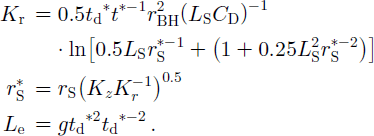
Here, g is gravitational acceleration, kz is vertical hydraulic conductivity, Le is effective borehole water-column length, lS and rS are length and radius of the equivalent screen, rBH is borehole radius, and td*t*-1 is the match-point ratio. This ratio is determined by reading corresponding (equal distance from the origin on both axes) times from the recorded (t*) and dimensionless (td*) time axes. Note that both the match-point ratio, tdt*- 1, and the dimensionless damping parameter, CD, depend on the scales used to plot the two time axes. This mutual dependence guarantees that the value of the horizontal hydraulic conductivity, k r, calculated from Equation (4), does not change with the scales of the time axes. The hydraulic conductivity ratio, kz kr- 1, must be estimated from independent considerations.
Results
At Bakaninbreen we focus on the underdamped slug-test responses recorded in one borehole upstream of the surge front (Fig. 1) in the 1995 summer melt season. Following an initial period of forced fluctuation, the response signal began oscillating in its natural frequency starting ∼8s after slug removal (Fig. 4a). Unfortunately, data collection was terminated before oscillations ceased, which was also the case for a repeat slug test conducted in this borehole. The signal-to-noise ratio for this repeat test was low because the initial water-level displacement was much smaller than during the initial test. We therefore do not include this response in the present study, but nevertheless note that analysis of this repeat test indicates that the results obtained from the initial slug test were reproducible.

Fig. 4. Analysis of the slug-test data collected at bakaninbreen: (a) raw data (black line) and background water-level change (grey line), and (b) water-level displacement corrected for background change (black line) and best-fit van der kamp type curve (grey line).
At midre Lovénbreen, slug tests were conducted in a total of five boreholes in the 2000 summer melt season. The slug-test responses recorded in four of these boreholes were characterized by high-frequency oscillations, which commonly indicates that the boreholes were hydraulically poorly connected or even unconnected to the subglacial aquifer (e.g. Reference Kulessa and HubbardKulessa and Hubbard, 1997; Reference KulessaKulessa, 2000). We therefore focus on the rising-head tests recorded in the remaining borehole, which were characterized by overdamped responses. Water-level monitoring during two out of the three repetitive slug tests conducted in this borehole was, unfortunately, terminated before the pre-test water level had fully recovered. We therefore focus on the remaining test for which a full dataset is available, but nevertheless note that comparison of the incomplete and complete water-level recoveries strongly suggests that the slug-test response was reproducible. The initial water-level displacement was ∼0.25 m, and the static water level was recovered after 4 100 s, allowing for a pronounced change in background level (Fig. 5a).

Fig. 5. Analysis of the slug-test data collected at midre lovénbreen: (a) raw data; (b) filtered data (black line) and background water-level change (grey line); and (c) normalized water-level displacement corrected for background change and time zero (black line) and best-fit Bulter- Garnett type curve (grey line).
Interpretation I: Bakaninbreen
Determination of subglacial hydraulic conductivity
Reference Stone, Clarke and EllisStone and others (1997) stressed the importance of removing background water-level changes from slug-test data recorded in glacier boreholes to avoid misinterpretation, which was confirmed by Reference Iken, Fabri and FunkIken and others (1996) and Reference KulessaKulessa (2000). Removal can be accomplished by fitting either a straight line (Reference Iken, Fabri and FunkIken and others, 1996; Reference Stone, Clarke and EllisStone and others, 1997; Reference KulessaKulessa, 2000) or polynomials (Reference Iken, Fabri and FunkIken and others, 1996) to the recorded background water-level changes, and subsequently subtracting the fitted curve from the dataset. At Bakaninbreen the background water-level change was corrected by subtracting the best-fit straight line from the raw dataset (Fig. 4a). The best-fit exponentially damped cyclic fluctuation was then calculated for and matched to the observed natural-frequency water-level oscillations using Equation (1) (Fig. 4b). Following earlier arguments, we have ignored the early, non-linear part of the response signal (e.g. Reference Van der KampVan der Kamp, 1976; Reference ButlerButler, 1997). The frequency and damping constant determined from curve matching are entered into Equation (2), together with the radius of the borehole, the radius of the equivalent screen, and the subglacial storage coefficient. This yields an estimate of the transmissivity of the sediment layer, which is converted to hydraulic conductivity using (e.g. Reference FetterFetter, 2001, p. 100)
In contrast to ground-water studies, the geometrical properties of the borehole–subglacial-aquifer flow system are commonly not well known in glaciological applications. We must therefore rely on best-guess estimates of these parameters in combination with rigorous sensitivity analysis. Our best-guess estimates of borehole radius (rBH = 0.05 m), equal to that used by all previous studies (e.g. Reference Stone and ClarkeStone and Clarke, 1993; Reference Iken, Fabri and FunkIken and others, 1996; Reference KulessaKulessa, 2000), equivalent screen radius (rS = 0.2 m), storage coefficient (s = 0.03) and sediment thickness (bSL = 0.5 m) are summarized in Table 1. Following earlier arguments, we set the radius and the length of the equivalent screen equal to the best estimates of the outer radius and the length of the skin (Reference Hyder, Butler, McElwee and LiuHyder and others, 1994).The diameter of the skin was chosen to be somewhat smaller than its length since the water jet acts predominantly in the vertical and downward direction. Reference Porter and MurrayPorter and Murray (2001) reported a specific storage of 0.064 m–1 for the sediment layer beneath Bakaninbreen, which is equivalent to a storage coefficient of ∼0.03 given a sediment thickness of 0.5 m (e.g. Reference FetterFetter, 2001, p.101). The best-guess sediment thickness (bSL) of 0.5 m is equal to the best estimate reported by previous studies, and specifically equals the length of the equivalent screen since the latter is assumed to fully penetrate the subglacial flow layer.
Table 1. Sensitivity analysis for Bakaninbreen

Entering these values into Equations (2) and (5), together with the parameters obtained from curve matching, gives a best-guess hydraulic conductivity of 8.2×10⁻³ ms–1 for the subglacial sediments beneath Bakaninbreen. Convergence of the computation with a residual error of 50.001% was achieved after 12 iterations.
Sensitivity analysis
We assume that the curve-fitting procedure involved in the Van der Kamp method is accurate compared to the best-guess estimates of borehole radius, radius and length of the skin, and anisotropy ratio (e.g. Reference KulessaKulessa, 2000). We therefore assigned each of the four uncertain parameters a maximum and a minimum value within the limits of reason, and varied each parameter individually relative to the best-guess estimates of the three remaining parameters. For a borehole radius of 0.03 m or less, an equivalent screen of 40.25 m and a storage coefficient of 0.05 or higher, the algorithm given in Equation (2) was found to be generally unstable, but in all other cases convergence with a residual error of 50.001% typically resulted after 515 iterations. Hydraulic conductivity changes resulting from this individualized sensitivity analysis were typically well within half an order of magnitude, except for the smallest storage coefficient (Table1). This value (1×10⁻⁷) is approximately equivalent to the specific storage reported for Gornergletscher (Reference Iken, Fabri and FunkIken and others, 1996). The standard error of the hydraulic conductivity range reported inTable 1 was calculated to be 7.9 × 10⁻³ m s–1.
We therefore conclude that the sediments beneath Bakaninbreen have a hydraulic conductivity of 8.2 ±7.9 × 10⁻³ ms–1.
Interpretation II: Midre Lovénbreen
Determination of subglacial hydraulic conductivity
A band-reject fast Fourier transform filter was applied to the raw data to eliminate disturbing frequencies between 0.5 and 10 Hz, allowing unequivocal identification of the initial water-level displacement (Fig. 5b). A consistent, non-linear background water-level change is superimposed on the recorded slug-test data (Fig. 5a), which is well approximated by a second-order polynomial (Fig. 5b). We thus remove the background water-level change by subtracting this second order polynomial from the dataset (Fig. 5b). The time-frame was adjusted by assigning time zero to the maximum water-level displacement. The data were then normalized with respect to this displacement, and matched to the best-fit Butler–Garnett type curve using the procedure described above (Fig. 5c). Independent confirmation for the goodness of the fit comes from the value of the effective water-column length calculated from the match-point ratio in Equation (4). This length was calculated to be 169 m, which is identical to the actual value of just over 169 m within the uncertainty pertaining to the best estimate of borehole depth (169.5 m).
The value for the dimensionless damping parameter (CD) and the match-point ratio (td*t*-1) obtained from curve matching are substituted into Equation (4), together with the geometrical properties of the borehole–subglacial-aquifer flow system. Our best-guess estimates of borehole radius ( rBH = 0.05 m), screen radius (rS = 0.5 m) and length (LS = 1.5 m), and anisotropy ratio (KzK–1=1) are summarized in Table 2. The choice of screen radius and length was guided by two main arguments. First, due to the significant depth of the borehole and the poorly defined ice–bed interface it was difficult to determine whether the drill had reached the glacier base. We appreciate that drill water could have been pumped into the subglacial substrate for up to ∼ 3 0 min. This would result in significant basal modifications, even if both the pressure and the temperature of this water were significantly reduced owing to the large depth. We specifically anticipate that the ice originally contained within the subglacial substrate was probably melted, and any fine sediment flushed away from the borehole base, while the coarse clasts probably largely remained in place. Taken together, these arguments lead us to expect that a considerable high-conductivity skin formed around the equivalent screen. In reference to earlier arguments, we again adjust the radius of the equivalent screen to the likely diameter of the high-conductivity skin, and choose this diameter to be somewhat smaller than screen length. Based on the length of time (≤ ∼ 3 0 min) during which drill water was pumped into the bed, and the reduced pressure and temperature of this water, we estimate the skin length to be ∼1.5 m, and the skin radius to be ∼0.5 m. The best-guess anisotropy ratio was chosen to be 1, assuming that the induced transient subglacial water flow was equal in all directions after correction for the high-conductivity skin.
Table 2. Sensitivity analysis for midre Lovénbreen

Substitution of the four best-guess geometrical and anisotropy values listed in Table 2 into Equation (4), together with the curve-matching parameters, gives a best-guess hydraulic conductivity estimate of 1.9 × 10– 5ms–1 for the clastic deposits beneath midre Lovénbreen.
Sensitivity analysis
As with the Bakaninbreen sensitivity analysis, we assume that the curve-fitting procedure involved in the Butler– Garnett method is accurate, which is in this case confirmed by matching calculated and observed effective water-column lengths. Again, each of the four uncertain parameters was varied individually within a reasonable range using the best-guess values for the three remaining parameters. The hydraulic conductivity changes were typically well within half an order of magnitude in all of these individualized cases (Table 2), with a standard error of 0.5 × 10⁻⁵ m s–1.
We therefore conclude that the hydraulic conductivity of the clastic deposits beneath midre Lovénbreen has a value of 1.9 i0.5 x10–5 ms– 1.
Synthesis and Conclusions
Our inferences suggest that the glacial till and marine sediments beneath Bakaninbreen have a hydraulic conductivity (8.2 ±7.8 × 10⁻³ms–1) that is almost three orders of magnitude larger than that of the clastic deposits beneath midre Lovénbreen (1.9 ± 0.5 × 10⁻⁵ ms–1). A marked discrepancy of more than one order of magnitude remains even if we assume a minimum hydraulic conductivity of 4.0 X10⁻⁴ ms– 1 for Bakaninbreen, and a maximum hydraulic conductivity of 2.4 × 10⁻⁵ ms–1 for midre Lovénbreen, as suggested by sensitivity analysis. This matches our initial observations based on the fact that underdamped and overdamped responses, respectively, reflect materials of high and low hydraulic conductivity (Reference Bredehoeft, Cooper and PapadopulosBredehoeft and others, 1966). We can now interpret our findings in the light of the other evidence collected at both glaciers.
If late-surge subglacial sediment deformation were absent, we would expect the hydraulic conductivity of the glacial till and marine sediments beneath Bakaninbreen to be noticeably smaller, and specifically to approximate textbook values (<10–6 m s–1; e.g. Reference FetterFetter, 2001, p. 85). Our findings are therefore consistent with, and provide unique field evidence of, marked hydraulic conductivity enhancement due to sediment dilation during the surge of Bakaninbreen. Significantly, our hydraulic conductivity estimate (8.2±7.8×10⁻³ m s–1) is several orders of magnitude larger than that reported by Reference Porter and MurrayPorter and Murray (2001) for the same sediments (∼10–7 to 10–8 ms–1) on the basis of long-term in situ borehole water-pressure and tilt-cell measurements. We agree with Reference Stone, Clarke and EllisStone and others (1997) that this discrepancy probably highlights the heterogeneous nature of the subglacial water system. We believe that at Bakaninbreen the glacier bed comprises a patchwork of dilated, transmissive regions of sediment interspersed with undilated, low-conductivity regions. Theborehole in which the slug tests were undertaken drained, suggesting that we intersected with dilated sediments. Compared to slug tests, long-term measurements are probably sensitive to larger regions of the bed including poorly transmissive sediment patches, resulting in an average, noticeably smaller hydraulic conductivity. Since Bakaninbreen had already slowed down when the present study and that of Reference Porter and MurrayPorter and Murray (2001) were conducted, it is likely that sediment dilation, and therefore also hydraulic conductivity enhancement, were less widespread than during times of peak or near-peak ice flow. We therefore suggest that the hydraulic conductivity values reported here (8.2±7.8×10⁻³ ms–1) could be common for widespread areas of the glacier bed during such times, while those inferred by Porter and Murray (∼10–7 to 10–8 ms–1) could be more typical during the quiescent phase.
We believe that our findings are consistent with the presence of coarse clasts, ice and interstitial water beneath midre Lovénbreen (E. King, unpublished data, 2000). The water-flow pathways within this form of permafrost can be expected to be predominantly small and poorly connected, supporting a small hydraulic conductivity (1.9±0.5×10⁻⁵ ms–1). Nevertheless, subglacial water evacuation is possible, and the magnitude of the hydraulic conductivity still appears large enough to prevent water from accumulating at the ice–permafrost interface. We noted earlier that four out of five boreholes did not connect, and argued that our experiences from drilling were consistent with regelation of basal ice into bed. It is therefore likely that many parts of the glacier are frozen to the bed. We believe that these arguments, taken together, provide compelling evidence that midre Lovénbreen is not capable of surging.
In summary, we have presented field evidence for significant hydraulic conductivity enhancement due to sediment dilation in the upper sediment horizon beneath a surging glacier. In contrast, the hydraulic conductivity of subglacial permafrost is comparatively small, despite the presence of coarse clastic deposits. The contrasting basal conditions beneath these two glaciers support the notion that midre Lovénbreen and other glaciers resting primarily on such deposits are not capable of surging (Reference Jiskoot, Murray and BoyleJiskoot and others, 2000).
Acknowledgements
This research was funded by grants from the U.K. Natural Environment Research Council (NERC; GT3/9031 and GST/02/2192). H. Vereecken (Research Center Julich, Germany) generously granted B.K. leave of absence in summer 2000, which made this study possible. A. Hiatt and P. Porter are thanked for their enthusiastic assistance with slug-test data collection in 1995. We received invaluable logistic support from M. Davey and N. Cox of the NERC Arctic Research Base during our 2000 season on midre Lovénbreen. We thank A. Smith and J. Kohler, and the Assistant Editor, H. Engelhardt, for helpful comments on the manuscript.


